Failure analysis of parameter-induced simulation crashes in climate models

(1)

Geosci. Model Dev., 6, 1157–1171, 2013 www.geosci-model-dev.net/6/1157/2013/ doi:10.5194/gmd-6-1157-2013

EGU Journal Logos (RGB)

Advances in

Geosciences

Open Access

Natural Hazards

and Earth System

Sciences

Open Access

Annales

Geophysicae

Open Access

Nonlinear Processes

in Geophysics

Open Access

Atmospheric

Chemistry

and Physics

Open Access

Atmospheric

Chemistry

and Physics

Open Access

Discussions

Atmospheric

Measurement

Techniques

Open Access

Atmospheric

Measurement

Techniques

Open Access

Discussions

Biogeosciences

Open Access Open Access

Biogeosciences

Discussions

Climate

of the Past

Climate

of the Past

Discussions

Earth System

Dynamics

Earth System

Dynamics

Discussions

Geoscientific

Instrumentation

Methods and

Data Systems

Open Access

_{Geoscientific}

Instrumentation

Methods and

Data Systems

Open Access

Discussions

Geoscientific

Model Development

Geoscientific

Model Development

Discussions

Hydrology and

Earth System

Sciences

Open Access

Hydrology and

Earth System

Sciences

Open Access

Discussions

Ocean Science

Discussions

Solid Earth

Discussions

The Cryosphere

Discussions

Natural Hazards

and Earth System

Sciences

Open Access

Discussions

Failure analysis of parameter-induced simulation crashes in

climate models

D. D. Lucas1, R. Klein1,2, J. Tannahill1, D. Ivanova1, S. Brandon1, D. Domyancic1, and Y. Zhang1

1_{Lawrence Livermore National Laboratory, Livermore, CA, USA}

2_{Department of Astronomy, University of California, Berkeley, CA 94720, USA}

Correspondence to: D. D. Lucas ([email protected])

Received: 3 January 2013 – Published in Geosci. Model Dev. Discuss.: 24 January 2013 Revised: 28 June 2013 – Accepted: 2 July 2013 – Published: 7 August 2013

Abstract. Simulations using IPCC (Intergovernmental Panel

on Climate Change)-class climate models are subject to fail or crash for a variety of reasons. Quantitative analysis of the failures can yield useful insights to better understand and im-prove the models. During the course of uncertainty quan-tification (UQ) ensemble simulations to assess the effects of ocean model parameter uncertainties on climate simula-tions, we experienced a series of simulation crashes within the Parallel Ocean Program (POP2) component of the Com-munity Climate System Model (CCSM4). About 8.5 % of our CCSM4 simulations failed for numerical reasons at com-binations of POP2 parameter values. We applied support vec-tor machine (SVM) classification from machine learning to quantify and predict the probability of failure as a function of the values of 18 POP2 parameters. A committee of SVM classifiers readily predicted model failures in an independent validation ensemble, as assessed by the area under the re-ceiver operating characteristic (ROC) curve metric (AUC>

0.96). The causes of the simulation failures were determined through a global sensitivity analysis. Combinations of 8 pa-rameters related to ocean mixing and viscosity from three different POP2 parameterizations were the major sources of the failures. This information can be used to improve POP2 and CCSM4 by incorporating correlations across the relevant parameters. Our method can also be used to quantify, predict, and understand simulation crashes in other complex geosci-entific models.

1 Introduction

Modern global three-dimensional climate models are ex-traordinarily complex pieces of science (e.g., Randall et al., 2007; Gent et al., 2011; The HadGEM2 Development Team, 2011) and software engineering (Easterbrook et al., 2011; Rugaber et al., 2011; Easterbrook, 2010). They contain over a million lines of code (Easterbrook and Johns, 2009; East-erbrook, 2012) and use hundreds to thousands of files, func-tions, and subroutines to solve equations of state and con-servation laws for the flows of matter, energy, and momen-tum within and between the atmosphere, oceans, land, and other reservoirs of the Earth system (Washington and Parkin-son, 2005). They also use numerous algorithms of biologi-cal, chemibiologi-cal, geologic, and anthropogenic processes to sim-ulate the cycles of carbon, nitrogen, sulfur, aerosols, ozone, greenhouse gases, and other climate-relevant quantities of in-terest. To compound this complexity, these algorithms oper-ate across many orders of magnitude in space and time, and contain constituents that exist in gas, liquid, solid and mixed phases.

(2)

1158 D. D. Lucas et al.: Failure analysis of climate simulation crashes

model validation). Varying amounts of software testing are conducted throughout the cycle, but formal code verification practices (e.g., see D’Silva et al., 2008) are only recently starting to be considered for climate model development (Clune and Rood, 2011; Farrell et al., 2011). Nonetheless, the concentration on sound science, as opposed to software correctness, has led to climate models that contain fewer soft-ware defects than other comparably sized projects (Pipitone and Easterbrook, 2012).

Software issues aside, many potential problems still arise with scientific representations in complex models. As code verification can be used to find software bugs, emerging tools being developed in the field of uncertainty quantifica-tion (UQ) (see Naquantifica-tional Research Council Report, 2012) can help pinpoint scientific discrepancies in simulation models, the knowledge of which can be used to guide and improve model development. Primary UQ targets for climate mod-els are schemes containing parameters with adjustable val-ues. These schemes represent physical processes that are not fully understood or cannot be directly simulated at the model resolutions of interest (e.g., Stensrud, 2009). Parameteriza-tions like this are often developed in isolation, so they can respond in unexpected ways when inserted in nonlinear cli-mate models and coupled to other parameterizations. Small perturbations to the values of the adjustable parameters can amplify and lead to large changes in simulation outputs. In some cases, the simulations may fail altogether.

We report here on a series of simulation crashes encoun-tered while running perturbed parameter UQ ensembles of the Community Climate System Model Version 4 (CCSM4) (Gent et al., 2011; CCSM4, 2012). Treating the simulation crash problem as a black box in which we know only the val-ues of the input parameters and a binary outcome flag indi-cating whether the simulations ultimately failed or were com-pleted, information that does not require detailed scientific knowledge, we present a method that successfully predicted crashes in independent simulations and pinpointed the model parameters that caused the failures.

Numerous studies have applied UQ techniques to cli-mate models similar to CCSM4 (e.g., Murphy et al., 2004; Stainforth et al., 2005; Jackson et al., 2008; Sanderson, 2011; Shiogama et al., 2012). However, analogous simulation fail-ures and crashes have been reported far less often, though we suspect that they occur more frequently than indicated by the relatively limited number of documented cases (i.e., a reporting bias). Failures, crashes, or bifurcations have been reported for climate models of both intermediate complex-ity (Webster et al., 2004; Annan et al., 2005; Edwards et al., 2011) and full complexity (see supplementary discussion in Stainforth et al., 2005). The failures in these cases were at-tributed to numerical instabilities, or to particular climate phenomena, such as the collapse of the Atlantic meridional overturning circulation or accelerated changes through pos-itive feedbacks in the models. Webster et al. (2004) and Edwards et al. (2011) present methods for calculating the

probability of failure for an input set of parameter values. In addition, Edwards et al. (2011) use the failure probabil-ity to design and prescreen ensemble members in follow-up ensembles.

Our analysis and approach are similar to Edwards et al. (2011), but with the added challenges of applying them to a climate model system that is computationally more demand-ing, uses smaller ensemble sizes, has more parameter uncer-tainty dimensions, and exhibits fewer simulation failures. To help overcome these challenges, we use machine learning al-gorithms to calculate and predict the failure probability. As climate models and other geoscientific codes become more complex and UQ studies more commonplace, we fully ex-pect parameter-induced simulation crashes to occur in these models with a greater frequency. Our failure analysis method will be beneficial for quantifying and determining the causes of these crashes.

2 Overview of climate simulations

Different sets of perturbed parameter UQ ensembles were executed as part of a broad effort to quantify and constrain uncertainties in the atmospheric, sea ice, and ocean model components of CCSM4 (Gent et al., 2011). The failures re-ported here occurred during simulations that perturbed pa-rameter values in the Parallel Ocean Program (POP2), the ocean component of CCSM4. For these experiments, POP2 was coupled with the sea ice model, while data-based compo-nents were used for the land and atmosphere. The simulations were integrated for 10 yr, and the system was forced with cli-matological air–sea flux data using normal year forcing from Large and Yeager (2009). Further details about POP2 and the UQ ensembles are given below.

2.1 Ocean model and parameters

POP2 is a state of the art depth-level model of the general ocean circulation that solves the 3-D primitive equations of rotational fluid dynamics and thermodynamics with standard approximations of Boussinesq and hydrostatics. It is devel-oped and maintained at Los Alamos National Laboratory (Smith et al., 2010) and is the ocean component of CCSM4 developed at the National Center for Atmospheric Research (Gent et al., 2011; Danabasoglu et al., 2012). The current simulations use the displaced-pole coordinate grid with the pole centered over Greenland and have a nominal horizontal resolution of 1◦_{. Vertically it resolves 60 depth levels with}

resolution varying from 10 m in the upper ocean (surface to 200 m) to 250 m in the deeper ocean. Refer to Smith et al. (2010) and Danabasoglu et al. (2012) for more information.

(3)

D. D. Lucas et al.: Failure analysis of climate simulation crashes 1159

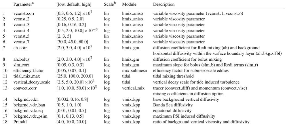
Table 1. Parameters sampled in the CCSM4 parallel ocean model.

Parametera [low, default, high] Scaleb Module Description

1 vconst corr [0.3, 0.6, 1.2]×107 lin hmix aniso variable viscosity parameter (vconst 1, vconst 6)

2 vconst 2 [0.25, 0.5, 2.0] log hmix aniso variable viscosity parameter

3 vconst 3 [0.16, 0.16, 0.2] lin hmix aniso variable viscosity parameter

4 vconst 4 [0.5, 2.0, 10.0]×10−8 log hmix aniso variable viscosity parameter

5 vconst 5 [2, 3, 5] lin hmix aniso variable viscosity parameter

6 vconst 7 [30.0, 45.0, 60.0] lin hmix aniso variable viscosity parameter

7 ah corr [2.0, 3.0, 4.0]×107 lin hmix gm diffusion coefficient for Redi mixing (ah) and background

horizontal diffusivity within the surface boundary layer (ah bkg srfbl)

8 ah bolus [2.0, 3.0, 4.0]×107 lin hmix gm diffusion coefficient for bolus mixing

9 slm corr [0.05, 0.3, 0.3] log hmix gm maximum slope for bolus (slm b) and Redi terms (slm r)

10 efficiency factor [0.05, 0.07, 0.1] lin mix submeso efficiency factor for submesoscale eddies

11 tidal mix max [25.0, 100.0, 200.0] log tidal tidal mixing threshold

12 vertical decay scale [2.5, 5.0, 20.0]×104 log tidal vertical decay scale for tide induced turbulence

13 convect corr [1.0, 10.0, 50.0]×103 log vertical mix tracer (convect diff) and momentum (convect visc)

mixing coefficients in diffusion option

14 bckgrnd vdc1 [0.032, 0.16, 0.8] log vmix kpp base background vertical diffusivity

15 bckgrnd vdc ban [0.5, 1.0, 1.0] lin vmix kpp Banda Sea diffusivity

16 bckgrnd vdc eq [0.01, 0.01, 0.5] log vmix kpp equatorial diffusivity

17 bckgrnd vdc psim [0.1, 0.13, 0.5] log vmix kpp maximum PSI induced diffusivity

18 Prandtl [4.0, 10.0, 20.0] log vmix kpp ratio of background vertical viscosity and diffusivity

a_Individual _corr_{parameters (numbers 1, 7, 9, and 13) are used to represent the correlated pair of parameters given in the description. For example, values drawn for}

vconst corrare assigned tovconst 1andvconst 6.bLinear and logarithmic scales are used for parameter ranges that have ratios of high/low<5and high/low≥5, respectively.

parameters and their uncertainty ranges are summarized in Table 1. Parameters 1–6 are used to capture horizontal mix-ing of momentum with spatially anisotropic viscosity (Large et al., 2001; Smith and McWilliams, 2003). Parameters 7– 9 are used for horizontal mixing of tracers via isopycnal eddy-induced transport (Gent and McWilliams, 1990). Pa-rameters 10–12 are used in recently developed schemes to simulate submesoscale and mixed-layer eddies (Fox-Kemper et al., 2008) and abyssal tidal mixing (Jayne, 2009). Parame-ters 13–18 are used for vertical convection and vertical mix-ing with the K-profile parameterization (KPP) scheme (Large et al., 1994).

2.2 UQ ensembles

Table 2 summarizes the UQ ensemble simulations. Three separate ensemble studies were conducted, each consisting of 180 simulations. The table also indicates the contributions of the studies to different types of analysis. For instance, stud-ies 1 and 2 were used to train machine learning algorithms to learn about simulation crashes (see Sect. 4.3), while study 3 was used to test the ability to predict simulation crashes (see Sect. 4.4). Out of 540 total simulations, there were 46 fail-ures, with the failures occurring at various times during the integration period. Each of the three studies used a Latin hy-percube method to sample the values of the 18 POP2 param-eters and a different random seed to generate the ensemble. The model parameters were represented using standard uni-form or log-uniuni-form probability distribution functions nor-malized to [0, 1] using the ranges (low and high values) and scales (linear and logarithm) noted in Table 1.

The Latin hypercube method is a stratified, space-filling variant of Monte Carlo sampling that is used extensively in UQ and uncertainty analysis (McKay et al., 1979; Helton and Davis, 2003). This sampling approach has superior vari-ance reduction properties over standard Monte Carlo sam-pling for some problems (Stein, 1987). For an ensemble size ofN, Latin hypercube splits each of theDparameter distri-butions intoN intervals of equal probability, resulting in a multi-dimensional grid withNDseparate bins. For our case,

D=18 andN=180. Ensemble members are obtained by selecting parameter values from different bins chosen at ran-dom, with the important constraint that the bins are cho-sen so that each interval along every parameter dimension is sampled only one time per ensemble. An example of a five-member Latin hypercube ensemble for two parameters is given by bins with indices (1, 4), (2, 2), (3, 5), (4, 3), and (5, 1), which is one of 120 valid possibilities for this config-uration. For our three UQ ensembles, the actual Latin hyper-cube sample points are illustrated in Figs. 1 and 2 for four of the POP2 parameters. These figures show that the Latin hy-percube sample point coverage is uniform and dense in one and two dimensions.

(4)

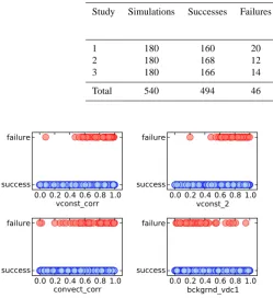
Table 2. Latin Hypercube Studies of the CCSM4 Parallel Ocean Program.

Study Simulations Successes Failures Failure rate Data used in Section

3 4.3 4.4 4.5 5

1 180 160 20 11.1 % X X X

2 180 168 12 6.7 % X X X

3 180 166 14 7.8 % X X X X

Total 540 494 46 8.5 %

Discussion

P

ap

er

|

Discussion

P

ap

er

|

Discussion

P

ap

er

|

Di

scuss

ion

P

ap

er

|

Table 2.Latin Hypercube Studies of the CCSM4 Parallel Ocean Program.

Study Simulations Successes Failures Failure rate Data used in Section 3 4.3 4.4 4.5 5

1 180 160 20 11.1 % X X X

2 180 168 12 6.7 % X X X

3 180 166 14 7.8 % X X X X

Total 540 494 46 8.5 %

0.0 0.2 0.4 0.6 0.8 1.0

vconst_corr

success

failure

0.0 0.2 0.4 0.6 0.8 1.0

vconst_2

success

failure

0.0 0.2 0.4 0.6 0.8 1.0

convect_corr

success

failure

0.0 0.2 0.4 0.6 0.8 1.0

bckgrnd_vdc1

success

failure

Fig. 1.Climate model simulation successes and failures are shown for one-dimensional projections of the values of 4 ocean parameters in 540 Latin hypercube experiments that sampled 18 model parameters. Parameter values are normalized using the ranges in Table 1.

28

Fig. 1. Climate model simulation successes and failures are shown for one-dimensional projections of the values of four ocean param-eters in 540 Latin hypercube experiments that sampled 18 model parameters. Parameter values are normalized using the ranges in Table 1.

incorporating observational data, performing statistical infer-ences, and estimating parameter values and probability dis-tributions using maximum likelihood and Bayesian methods. Of the many capabilities provided by the UQ Pipeline, the failure analysis presented here uses the simulation parameter values and a method for calculating parameter sensitivities.

3 Descriptive failure analysis

Figures 1 and 2 show simulation successes and failures for the three Latin hypercube studies (540 runs) as a function of the values of 4 of the 18 parameters sampled in POP2. Sim-ilar figures were generated for the other parameters, but are not displayed to keep the discussion brief and because the failures are highly sensitive to changes in these parameters (see Sect. 5). It is not possible to directly visualize the depen-dencies in high dimensions, so the figures show the outcomes projected in one and two parameter dimensions (Figs. 1 and 2, respectively).

From the figures it is clear that the failures are gen-erally concentrated around high values of parameters

vconst corr and vconst 2, and at low values of

backgrnd vdc1. A weaker dependence of the failures on

Discussion

P

ap

er

|

Discussion

P

ap

er

|

Discussion

P

ap

er

|

Di

scuss

ion

P

ap

er

|

0.0 0.2 0.4 0.6 0.8 1.0

vconst_corr

0.0

0.2 0.4 0.6 0.8 1.0

vconst_2

0.0 0.2 0.4 0.6 0.8 1.0

vconst_corr

0.0

0.2 0.4 0.6 0.8 1.0

convect_corr

failure success

0.0 0.2 0.4 0.6 0.8 1.0

vconst_corr

0.0

0.2 0.4 0.6 0.8 1.0

bckgrnd_vdc1

0.0 0.2 0.4 0.6 0.8 1.0

vconst_2

0.0

0.2 0.4 0.6 0.8 1.0

convect_corr

0.0 0.2 0.4 0.6 0.8 1.0

vconst_2

0.0

0.2 0.4 0.6 0.8 1.0

bckgrnd_vdc1

0.0 0.2 0.4 0.6 0.8 1.0

convect_corr

0.0

0.2 0.4 0.6 0.8 1.0

bckgrnd_vdc1

Fig. 2.Same as Fig. 1, but showing the two-dimensional projections for the same four model parameters.

31

Fig. 2. Same as Fig. 1, but showing the two-dimensional projections for the same four model parameters.

high values ofconvect corris also apparent. The analy-sis presented in following sections does not require a detailed understanding of the physical reasons that connect parameter values to simulation failures, though we briefly summarize the connections to help with the interpretation.

(5)

(Large et al., 1994). Reducing the values ofbckgrnd vdc1

and otherbckgrndparameters increase the numerical noise in the solution and consequently cause numerical instability. Similarly, increasing the value ofconvect corr, which increases diffusivity and viscosity in the implicit KPP verti-cal mixing scheme, leads to instabilities in the vertiverti-cal den-sity profile. For detailed descriptions of all of the POP2 pa-rameters used in the current study, please refer to Smith and McWilliams (2003), Large et al. (2001), and Danabasoglu et al. (2012).

In spite of the obvious relationships between the param-eter values and simulation outcomes, other features present in the figures suggest that the ability to determine the causes of the failures is potentially complicated. Figure 2, for in-stance, indicates that there are strong correlations between failed simulations and pairs of parameter values. As one example, failures occur at the combination of high values of vconst corr and low values of backgrnd vdc1. These two parameters reside in different modules in POP2 (hmix aniso, andvmix kpp, respectively), which makes it difficult for POP2 model developers and users to discover and attribute simulation failures to correlations in these pa-rameters.

A more important complication arises from the overlap of simulation successes and failures in the low dimensional pro-jections shown in the figures. Some simulations appear to fail in the same general vicinity of parameter space where other simulations succeed, and vice versa. To illustrate, the upper right portion of the scatterplot betweenvconst corrand

vconst 2in Fig. 2 contains a high density of failures and successes. Another notable example is the isolated failure event shown in the lower left hand corner of the same scat-terplot.

These overlaps can lead to serious misclassification errors in statistical models used to predict failures as a function of parameter values. Two types of misclassification errors can occur. Simulations that are predicted to fail, but actually suc-ceed are false positives or type I errors; those that are pre-dicted to succeed, but actually fail are false negatives or type II errors (see Sect. 4 for further details). Imbalanced data, in which the population of one class greatly outnumbers the populations of other classes, are associated with class over-lap (Prati et al., 2004), and the POP2 outcomes are highly imbalanced (i.e., 46 failures out of 540 simulations). Another related explanation is that higher parameter dimensions, and possibly a non-linear decision boundary, are required to ef-fectively separate the outcomes.

Statistical approaches more powerful than the descriptive relationships illustrated in Figs. 1 and 2 are therefore needed to attack our problem. As described in the remaining sec-tions, we turned to algorithms and diagnostics developed in the fields of pattern recognition, machine learning, and sig-nal detection. These methods provided us with the ability to predict simulation failures in advance of running the model and a tool to quantify the causes of the failures. This latter

capability can be used to improve POP2 by making it more robust to parameter changes.

4 Probabilistic failure classification

For a given set of model input parameters, a POP2 simula-tion will either succeed or fail. We denote these outcomes by a two-class categorical variable in which failures belong to classCfand successes belong to classCs. The present

discus-sion considers only a single failure class, but we recognize that simulations can fail for a variety of reasons (e.g., lack of iterative convergence, numerical instabilities, etc). Without difficulty, the two-class methodology described below can be extended to handle multiple modes of failure through multi-class multi-classification.

Our goal for probabilistic failure classification is to de-termine the probability that a POP2 simulation will fail for a vector of model input parametersx=(x1, x2, . . . , x18). We

denote this using the conditional probabilityP(Cf|x). Using

Bayes’ rule, the posterior conditional probability can be writ-ten

P(Cf|x)=

P(x|Cf)P(Cf)

P(x|Cf)P(Cf)+P(x|Cs)P(Cs)

, (1)

where P(x|Ci) and P(Ci) correspond to class-conditional densities and class priors, respectively. By introducing a vari-ableλrepresenting the natural logarithm of the likelihood-odds ratio,

λ=ln _P_(x_|_C

f)

P(x|Cs) P(Cf) P(Cs)

, (2)

Eq. (1) can be rewritten as the “S-shaped” logistic sigmoid function

P(Cf|x)=

1

1+exp(−λ). (3)

Theλterm is a function ofx and takes values in(−∞,∞). As illustrated in Fig. 3, the sigmoid function is bounded be-tween 0 and 1, inclusive. This formalism provides a mecha-nism to transform an input vector of model parameter values to a probability that the corresponding simulation will fail or succeed.

(6)

Discussion

P

ap

er

|

Discussion

P

ap

er

|

Discussion

P

ap

er

|

Di

scuss

ion

P

ap

er

|

10 5 0

_x

5 10

0.0

0.2

0.4

0.6

0.8

1.0 Failure Probability

Fig. 3.Logistic sigmoid function defined in Eq. (3) withλ(x) =x.

32

Fig. 3. Logistic sigmoid function defined in Eq. (3) withλ(x)=x.

Discussion

P

ap

er

|

Discussion

P

ap

er

|

Discussion

P

ap

er

|

Di

scuss

ion

P

ap

er

|

Feature Space

kernel transformation

Input Parameter Space

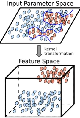
Fig. 4.Conceptual image showing the separability of the red and blue classes through kernel transfor-mations in SVMs.

33

Fig. 4. Conceptual image showing the separability of the red and blue classes through kernel transformations in SVMs.

case would “fail” by simulating temperatures that exceed the 5 K threshold, information that developers could use to im-prove their models.

4.1 SVM classification

Support vector machine (SVM) classification (Vapnik, 1995; Cortes and Vapnik, 1995; Burges, 1998) from the fields of pattern recognition and supervised machine learning (Bishop, 2007; Kotsiantis, 2007) is used to assign a simula-tion to classCforCsfor input vectorx. This type of

classifica-tion problem can also be handled using other methods, such as logistic regression (Hosmer and Lemeshow, 2000), neu-ral networks (Bishop, 2007), decision trees (Breiman et al., 1984), and random forests (Breiman, 2001). We limit our at-tention to SVMs, however, given our familiarity with the al-gorithm and its excellent performance on our climate model application.

Briefly, the SVM method is based on maximizing the dis-tance between parallel hyperplanes that separate the classes (i.e., the margin), while allowing for misclassifications from overlapping data points during training (i.e., a soft mar-gin). For non-linearly separable classes, the hyperplanes are determined by transforming the input space to a higher-dimensional feature space using kernel functions. The pur-pose of the transformation is to make it easier to separate the classes, as illustrated conceptually in Fig. 4. The support vec-tors are the training points that lie on the margin for classes that are separable, and lie on or within the margin for classes that are not. New input vectorsxare assigned to a class using the sign of the predictive decision function:

f (x)=

Ns

X

i=1

yiαiK(xi,x)+b, (4)

wheref (x) >0 andf (x) <0 are assigned to classesCfand Cs, respectively. The sum in Eq. (4) is over theNs support

vectors from the training set,yi∈ {−1,1} is a binary out-come indicator variable,K(xi,x)is the kernel function, and

bandαiare, respectively, bias and Lagrange multiplier terms determined through constrained optimization of the margin. Refer to Burges (1998), Bishop (2007), or Chang and Lin (2011) for further details.

The decision function in Eq. (4) assigns inputs to a class, but does not provide a probability of class membership. An extension to the standard SVM approach was therefore devel-oped (Platt, 1999) that derives class probabilities by fitting

λin Eq. (2) to a two parameter function using the training data and cross validation. A variation of this procedure is im-plemented in theLIBSVMpackage (Chang and Lin, 2011), which we used to fit SVM classifiers that calculate the failure probabilitiesP(Cf|x).

As described in more detail in Sect. 4.3, we also applied an ensemble learning approach (Dietterich, 2000) to create a “committee” of SVM classifiers. Each classifier in the com-mittee contributes a vote (i.e., failure probability), and the votes are tallied in different ways to predict simulation fail-ures and to assess the performance of the classification sys-tem.

4.2 Classification performance

(7)

Discussion

P

ap

er

|

Discussion

P

ap

er

|

Discussion

P

ap

er

|

Di

scuss

ion

P

ap

er

|

Actual

Fa

ilu

re

S

u

cc

e

ss

Failure Success

True Positive

(TP)

False Negative

(FN)

False Positive

(FP)

True Negative

(TN)

TPR =

TP/(TP+FN) FP/(FP+TN)FPR =

P

re

d

ic

te

d

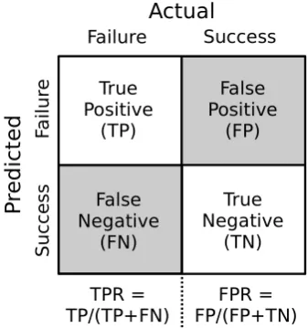
Fig. 5. The confusion matrix showing the four possible outcomes for a two-class simulation failure

problem.

34

Fig. 5. The confusion matrix showing the four possible outcomes for a two-class simulation failure problem.

TPR= TP

TP+FN, (5)

and

FPR= FP

FP+TN. (6)

Perfect classifiers have TPR and FPR values of 1 and 0, re-spectively. As noted previously, we use SVM classifiers that provide probabilities of class membership. The assignment to a particular class, and resulting TPR and FPR values, there-fore depends upon a specified decision variable and threshold value. If decisions are made using the failure probability with a threshold of 0.5, for example, then probabilities above and below this threshold will be assigned to classesCf andCs,

respectively.

The quantities in Eqs. (5) and (6) are combined into a con-venient diagram used in signal detection and decision analy-sis known as a receiver operating characteristic (ROC) curve (Swets, 1988; Fawcett, 2006). ROC curves plot the FPR (hor-izontal axis) versus TPR (vertical axis) of a decision variable as the threshold is varied from+∞to−∞. A perfect classi-fier is represented in ROC space by the vertical line connect-ing points (0, 0) and (0, 1), followed by the horizontal line connecting points (0, 1) and (1, 1). A classifier that makes random assignments, on the other hand, is represented by the diagonal line connecting points (0, 0) and (1, 1). The predic-tive capability of a classification system can therefore be as-sessed by a single number, the area under the ROC curve (AUC) (e.g., Marzban, 2004). As a rough rule of thumb, a classifier with an AUC score of about 0.8 or higher is useful for discrimination. The AUC score is used in following sec-tions to train SVM classifiers and to test their performance on independent simulation failure data.

Table 3. Predictions and outcomes of simulation crashes in study 3.

Run µc σc Predicted∗ Actual Davg Dsum Dsnr

002 0.47 0.13 Success Failure Success Success 006 0.54 0.14 Failure Failure Failure Failure 015 0.37 0.10 Success Success Failure Success 017 0.42 0.12 Success Failure Failure Failure 027 0.25 0.09 Success Success Success Failure 044 0.04 0.02 Success Success Success Failure 060 0.80 0.10 Failure Failure Failure Failure 073 0.52 0.15 Failure Failure Failure Failure 088 0.63 0.11 Failure Failure Failure Failure 095 0.47 0.15 Success Failure Success Success 097 0.83 0.09 Failure Failure Failure Failure 120 0.49 0.13 Success Failure Failure Failure 141 0.88 0.09 Failure Failure Failure Success 148 0.76 0.12 Failure Failure Failure Failure 155 0.31 0.08 Success Success Failure Failure 166 0.64 0.11 Failure Failure Failure Failure 173 0.75 0.12 Failure Failure Failure Failure 177 0.67 0.14 Failure Failure Failure Failure

∗_{Actual successes predicted by all decision criteria are not reported here for the sake}

of brevity. Predictions fromDavgandDsumwere made before the study, while those

fromDsnrwere determined retrospectively.

4.3 Supervised learning of simulation failures

The three UQ studies listed in Table 2 were performed in suc-cession to one another. After completing studies 1 and 2, but before starting study 3, we trained a committee of SVM clas-sifiers to learn about the simulation failures. The goal was to use the committee to predict the outcomes of study 3 before those simulations even began to run. This section describes the training procedure, while the following two sections de-scribe the performance on study 3.

The training set consisted of the 360 simulations from studies 1 and 2, which had 32 simulation failures and 328 successes. Given the relatively small ratio of the number of failure events to the number of classifier inputs (i.e., 32 / 18), we utilized an ensemble learning approach (Dietterich, 2000) known as bootstrap aggregation (i.e., “bagging”) (Breiman, 1996). Bagging quantifies the variability of classifier predic-tions and can help improve the overall classification perfor-mance. The bagging was applied by resampling the training dataNb=100 times, allowing for duplicates in the samples

(i.e., sampling with replacement). This step effectively cre-ated 100 different versions of the training data that were used to construct the committee of individual SVM classi-fiers. Failure predictions were then made by aggregating the votes across the committee, using an equal weight for each classifier. In particular, we computed the mean value (µc) and

(8)

µc=

1

Nb

X

i=1

Pi(Cf|x) (7)

and

σ_c2= 1 Nb

Nb

X

i=1

[Pi(Cf|x)−µc]2, (8)

and then combined these quantities in different ways to form decision variables for prediction and ROC analysis (see Sects. 4.4 and 4.5).

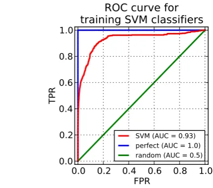
The LIBSVMpackage (Chang and Lin, 2011), which is freely available and open source, was used to train each of the classifiers in the committee.LIBSVMoffers two versions of SVM classification (C-support andν-support) and four stan-dard types of kernel functions (linear, polynomial, Gaussian, and hyperbolic tangent). On the basis of familiarity and ex-perience, we employedC-support classification with Gaus-sian kernels,K(xi,x)=exp(−γkxi−xk2), though we sub-sequently tested other kernels (see below). The values of two adjustable SVM-related parameters, the kernel widthγ and misclassification penaltyC, were determined using a cross validation method (Arlot and Celisse, 2010). For each boot-strap replicate of the training dataset, we randomly selected 80 % of the data to construct an individual classifier and used the remaining 20 % to test that classifier. The objec-tive was to find values forγ andC that are the same for all of the classifiers and that maximize their performance on these held-out tests. This task was accomplished by com-bining the individual tests into a large cross validation test set with 7200 data instances (0.2 test fraction×360 simula-tions×100 resampling size), and then computing the ROC curve and AUC score on this data. Figure 6 shows the ROC curve using the values that maximized the AUC (γ=0.1,

C=3, and AUC=0.93). The area under the curve is well above 0.8, which indicated that the SVM committee could be used for predicting simulation crashes in study 3.

The analysis presented throughout the manuscript utilized only the Gaussian kernels. However, to test the sensitivity to the choice of SVM kernel, we subsequently re-trained the classifiers using the same training data and cross validation technique, but instead applied linear, cubic, and hyperbolic tangent kernel functions. The Gaussian kernels performed slightly better than the other kernels, but all of the kernels still achieved cross validation AUC scores above 0.92. This test suggests that theCfandCs classes are primarily linearly

separable, because the linear kernel performed nearly as well as the nonlinear kernels.

4.4 Predicting simulation failures

Before running the 180 simulations in study 3, we used the SVM classifier committee trained from studies 1 and 2 to predict simulation failures in study 3. These predictions were

Discussion

P

ap

er

|

Discussion

P

ap

er

|

Discussion

P

ap

er

|

Di

scuss

ion

P

ap

er

|

0.0 0.2 0.4 0.6 0.8 1.0

FPR

0.0

0.2

0.4

0.6

0.8

1.0 TPR

ROC curve for

training SVM classifiers

SVM (AUC = 0.93)

perfect (AUC = 1.0)

random (AUC = 0.5)

Fig. 6.Receiver operating characteristic for the bootstrapped set of individual SVM classifiers assessed using holdout test data. SVM training parameters (γ= 0.1,C= 3) are chosen to maximize the area under the ROC curve.

35

Fig. 6. Receiver operating characteristic for the bootstrapped set of individual SVM classifiers assessed using holdout test data. SVM training parameters (γ=0.1,C=3) are chosen to maximize the area under the ROC curve.

sent out to group members by email at the beginning of the study (see fourth and fifth columns in Table 3) and were largely validated by the end of the study. The predictions were based on Eqs. (7) and (8). Simulations were assigned to theCfclass using decision criteria denoted by

D≡decision variable≥threshold. (9) Two initial criteria were selected using the same threshold, but different decision variables. The first criterion used the committee average,

Davg≡µc≥0.5, (10)

while the second used the sum of the committee average and standard deviation,

Dsum≡µc+σc≥0.5. (11)

The second criterion was chosen to account for variability across committee members by categorizing some simulations as Cf even though they had a committee mean below 0.5.

After all of the simulations were completed, a third criterion based on the signal-to-noise ratio from the committee,Dsnr,

was also considered and analyzed (see Sect. 4.5).

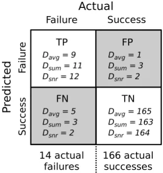
The predictions and actual outcomes are summarized in Table 3 and displayed in Figs. 7 and 8. As noted in Table 2, there were 14 actual simulation failures and 166 successes in the study. The classifier committee performed exceedingly well using the two initial criteria,Davg andDsum. Referring

(9)

Discussion

P

ap

er

|

Discussion

P

ap

er

|

Discussion

P

ap

er

|

Di

scuss

ion

P

ap

er

|

Actual

Fa

ilu

re

S

u

cc

e

ss

Failure Success

TP

14 actual

failures 166 actual successes

P

re

d

ic

te

d

DDavg_sum = 9 = 11 D_snr = 12

FP

D_avg = 1 D_sum = 3 D_snr = 2

FN

Davg = 5 D_sum = 3 Dsnr = 2

TN

Davg = 165 D_sum = 163 Dsnr = 164

Fig. 7. The confusion matrix for predictions of 180 simulations in study 3 using the SVM committee

with three different decision criteria (Davg,Dsum, andDsnr).

36

Fig. 7. The confusion matrix for predictions of 180 simulations in study 3 using the SVM committee with three different decision cri-teria (Davg,Dsum, andDsnr).

FNs than FPs, whileDsumhad an equal number of each.

Be-cause of this difference,DavgandDsumoperate at different

points in ROC space.Davghas ROC coordinates of (1/166,

9/14), whileDsumoperates at (3/166, 11/14). Based on their

Euclidean distance from a perfect classifier, which is given by FPR2+(TPR−1)21/2, we conclude that Dsum

(dis-tance=0.215) performs better thanDavg(distance=0.357).

To ascertain the cause of the performance difference be-tweenDsum andDavg, the top and middle panels in Fig. 8

display the actual outcomes and predictions using theµcand

µc+σc decision variables for the runs in study 3. The

de-cision criteria are represented by the horizontal lines in the panels. Runs that are on or above the lines were predicted to fail, while those below were predicted to succeed. Cor-rect predictions are displayed in blue (TP and TN), and in-correct predictions in red (FP and FN). The figure indicates, for example, that runs 17 and 120 failed, but were misclas-sified byDavg because their µc values were slightly below

0.5. By comparisonDsumassigned these runs to the correct

class, but also misdiagnosed runs 2 and 95. A visual inspec-tion of the figure shows that, except for the relative posiinspec-tion of the threshold, the distribution of points inµcandµc+σc

look very similar. We therefore attribute the performance dif-ference to the threshold value. IfDavghad used a threshold

value of about 0.4 instead of 0.5, it would have made the same predictions and had the same performance asDsum.

At this point, we can also compare the predictive perfor-mance of our classification system to the “second design” predictions in Edwards et al. (2011) (see Sect. 4.3 therein). We do not compare to their “first design” results (i.e., the ta-ble of Sect. 4.2 therein), because those results use the same data to both train and evaluate their statistical model (i.e., they are not predictions). Moreover, Edwards et al. (2011) provide only TN and FN values for this design because they

screened out simulations that were predicted to fail. Their model incorrectly classified 26 % of the predicted successes, which we calculate using FN/(FN+TN). By comparison, our system misclassified only 3 and 2 % of the predicted suc-cesses usingDavgandDsum, respectively.

4.5 Retrospective analysis of simulation failures

After study 3 was completed, we applied the same SVM committee to test the performance of an additional crite-rion based on the signal-to-noise ratio, µc/σc, as the

deci-sion variable. Without prior knowledge about a setting for the threshold for this criterion, it was not used to predict simula-tion failures in advance. Retrospectively, we used the same values of µc andσc that were used for the predictions in

Sect. 4.4, but determined and tested a setting for the threshold that maximizes the overall accuracy and minimizes the total number of false outcomes (FP+FN). The resulting criterion is defined by

Dsnr≡µc/σc≥3.53. (12)

The performance of this criterion is displayed in Table 3 and Figs. 7 and 8. As shown,Dsnr outperforms bothDavg

andDsum. If included in our set of predictions, this criterion

would have made 176 correct predictions (97.8 % accuracy) and only four false predictions balanced between two FNs (runs 27 and 44) and two FPs (runs 15 and 141). Dsnr

op-erates at ROC point (2/166, 12/14), which is a distance of 0.143 from a perfect classifier. The reason for the improved performance is shown more clearly in Fig. 8. The signal-to-noise ratio better separates the failures and successes than ei-ther of the oei-ther decision variables, although runs 44 and 141 are still grossly misclassified. In spite of the improvement, it is also worth noting that more simulations lie closer toDsnr

than eitherDavgorDsum. This implies that the performance

ofDsnris more sensitive to slight adjustments in the value of

the threshold than the other criteria.

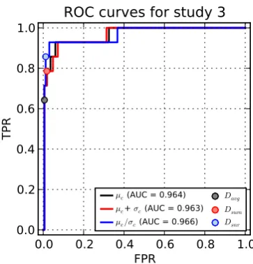
In retrospect, we also varied the thresholds for the three decision variables and calculated the FPRs and TPRs for study 3. The resulting ROC curves and fixed locations of the decision criteria are shown in Fig. 9. The ROC curves forµcandµc+σcnearly overlap, which confirms the

previ-ous statement that these two decision variables perform sim-ilarly after accounting for threshold differences. Based on their AUC scores,µcperforms marginally better thanµc+σc

because adding committee variability causes some success-ful simulations to get tallied relatively sooner as FPs (see points with values close to run 27 in Fig. 8). In contrast to these cases, the ROC curve forµc/σcis noticeably better and

has an AUC of 0.966. This occurs becauseµc/σcis more

(10)

1166 D. D. Lucas et al.: Failure analysis of climate simulation crashes _Discussion P ap er | Discussion P ap er | Discussion P ap er | Di scuss ion P ap er |

0.0

0.2

0.4

0.6

0.8

1.0 µ

c 1 2 3 4 5 6 7 8

910111213

14

15

16

17

18

192021

22 2324 25 26 27 28 29 30 31 32 33 34 3536 37 38 39 40 41

42434445

46

47

484950 51525354

55

5657

58

59

60

61626364

65

66

67

686970

71 72 73 74 75 76

777879

80 81 82 8384 85 86 87 88

899091

92 93 94 95 96 97

9899100101102

103 104 105 106 107108 109 110 111 112 113 114115 116 117 118 119 120 121 122

123124125

126

127128129130131

132 133 134135 136 137138 139 140 141 142143 144145 146 147 148

149150151152

153 154 155 156 157 158 159 160 161 162 163 164 165 166

167168169170171

172 173 174175 176 177 178 179180

D

avg

true positive false positive true negative false negative

0.0

0.2

0.4

0.6

0.8

1.0 µ

c

+

σ

c 1 2 3 4 5 6 7 8 910 111213

14

15

16

17

18

192021

22 2324 25 26 27 28 29 30 31 32 33 34 3536 37 38 39 40 41 4243 44 45 46 47

484950 51525354

55

5657

58

59

60

61626364

65 66 67 68 6970 71 72 73 74 75 76 7778 79 80 81 82 8384 85 86 87 88

899091

92 93 94 95 96 97

9899100101102

103 104 105106 107108 109 110 111 112 113 114115 116 117 118 119 120 121 122 123124 125 126

127128129130131

132 133 134135 136 137138 139 140 141 142143 144145 146 147 148

149150151152

153 154 155 156 157 158 159 160 161 162 163 164 165 166

167168169170171

172 173 174175 176 177 178 179180

D

sum

Decision variable

1

30

60

90

120

150

180 Study 3 run number

0

2

4

6

8

10 µ

c

/σ

c 1 2 3 4 5 6 7 8 910 11 12 13 14 15 16 17 18 19 20 21 22 23 24 25 26 27 28 29 3031 32 33 34 35 36 37 38 39 40 41 42 4344 45 46 47 48 4950 51 52 53 5455 5657 58 59 60 6162 6364 65 66 67 68 69 70 71 72 73 74 75 76 77 78 7980 81 82 83 84 85 86 87 88 89 90 91 92 93 94 95 96 97 98 99100 101 102 103 104 105 106 107108 109 110 111 112 113 114 115 116 117 118 119 120 121 122 123 124 125 126 127 128 129 130 131 132 133 134 135 136 137 138 139 140 141 142 143 144 145 146 147 148 149 150151 152 153 154 155 156 157 158 159 160 161 162 163 164 165 166 167 168

169170171

172 173 174 175 176 177 178 179 180

D

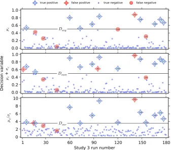
snr

Fig. 8. Actual and predicted outcomes are shown for the 180 simulations in study 3. Predictions are based on three decision variables and thresholds(µcandDavg, top;µc+σcandDsum, middle;µc/σcand

Dsnr, bottom). The horizontal axis displays simulation numbers based on their order in the ensemble.

Simulation failures and successes are shown using stars and circles, respectively. Correct and incorrect predictions are shown in blue and red, respectively.

37

Fig. 8. Actual and predicted outcomes are shown for the 180 simulations in study 3. Predictions are based on three decision variables and thresholds (µcandDavg, top;µc+σcandDsum, middle;µc/σcandDsnr, bottom). The horizontal axis displays simulation numbers

based on their order in the ensemble. Simulation failures and successes are shown using stars and circles, respectively. Correct and incorrect predictions are shown in blue and red, respectively.

consider the tradeoffs between TPs and FPs. Slightly lower-ing the threshold inDsnr, for example, will increase the TPR

and move it to a point that lies closer to a perfect classifier in ROC space, but this occurs at the expense of also increasing the FPR.

5 Sensitivity analysis of simulation failures

Following on the demonstrated success of our predictions, we used the classifier committee to identify, quantify, and rank the importance of the model parameters responsible for the simulation failures. This information can be used to make the model more robust to parameter perturbations by improv-ing the modules associated with the most sensitive parame-ters. For this analysis, we drew 104 Latin hypercube sam-ples from uniform distributions representing the 18 POP2 parameters, calculated the average failure probability from a committee of SVM classifiers (µc) at each of the

sam-ple points, and then performed a global sensitivity analysis (Saltelli et al., 2000; Helton et al., 2006) on the parameter-induced variance of log µc. All of the available simulation

data were used to compute the parameter sensitivities by

re-training a new committee of 100 SVM classifiers with the full set of 540 simulations from studies 1–3. The training fol-lowed the procedure previously described in Sect. 4.3. Also note that the sensitivity analysis is illustrated below usingµc

as the committee response, but the same general results are obtained using the signal-to-noise ratio (µc/σc).

5.1 Polynomial chaos expansion of the failure probability

Parameter sensitivities were measured and ranked using Sobol indices (Sobol, 2001; Saltelli et al., 2000), which decompose the variance of log µc into contributions from

individual parameters and various higher-order combinations of parameters. Polynomial chaos expansions (Wiener, 1938) provide a convenient format for the sensitivity analysis be-cause the squares of the expansion coefficients are directly proportional to Sobol indices (Sudret, 2008; Lucas and Prinn, 2005; Tatang et al., 1997). The distribution of log µc was

fit toNp=18 parameters using a second-order polynomial

(11)

logµc=a0+

Np

X

i=1

[biP1(ξi)+ciP2(ξi)]

+

Np−1

X

i=1

Np

X

j=i+1

dijP1(ξi)P1(ξj), (13)

whereξi is the random variable representation of parameter

i,Pn(ξi)is ann-th order orthogonal polynomial inξi, and the

a0,bi,cianddij are expansion coefficients to be determined. For the case where theξi are standard uniform random vari-ables, thePn(ξi)are the shifted Legendre polynomials (see Xiu and Karnidakis, 2002) with the following orthogonality property:

1

Z

0

Pm(ξi)Pn(ξi)dξi = 1

2n+1δmn, (14)

whereδmnis the Kronecker delta function. The first and sec-ond order shifted Legendre polynomials are given by

P1(ξi)=2ξi−1 (15) and

P2(ξi)=6ξi2−6ξi+1. (16) The coefficients in Eq. (13) were determined through least squares, and higher-order terms were not considered because the second-order expansion fits the data very well (adjusted

R2=0.98). The resulting fit is given in Table 4, which shows the leading terms of the expansion in two forms.

Analytical expressions for the moments of log µc as

a function of the POP2 parameters were derived by directly taking expectation values of Eq. (13). The average value and variance are

avg(logµc)=a0, (17)

and

var(log µc)=

individual parameters

z }| {

Np

X

i=1

b2_i

3 +

c_i2

5 !

+

pairs of parameters

z }| {

Np−1

X

i=1

Np

X

j=i+1

d_ij2

9 . (18)

The two groups of terms labeled on the right hand side of Eq. (18) signify variance contributions from individual pa-rameters (linear and quadratic) and pairs of papa-rameters. The fractional values of the squared polynomial chaos expansion coefficients in Eq. (18) follow from application of Eq. (14).

5.2 Sensitivity network of the failure probability

Given a parameter-based decomposition of the variance, we have developed a technique to visualize complex variance

Discussion

P

ap

er

|

Discussion

P

ap

er

|

Discussion

P

ap

er

|

Di

scuss

ion

P

ap

er

|

0.0 0.2 0.4 0.6 0.8 1.0

FPR

0.0

0.2

0.4

0.6

0.8

1.0 TPR

ROC curves for study 3

µc (AUC = 0.964) µc+ σc (AUC = 0.963) µc/σc (AUC = 0.966)

Davg Dsum Dsnr

Fig. 9. ROC curves for the 180 simulations in study 3 using the SVM committee with three decision

variables (µc,µc+σc, andµc/σc). The locations of the discriminators using the fixed thresholds inDavg,

Dsum, andDsnrare also shown.

38

Fig. 9. ROC curves for the 180 simulations in study 3 using the SVM committee with three decision variables (µc, µc+σc, and µc/σc). The locations of the discriminators using the fixed

thresh-olds inDavg,Dsum, andDsnrare also shown.

connections using network graphs with nodes and edges. The size of nodei in the graph is proportional to the fractional contribution from parameteri,

nodei∝

b2_i/3+c2_i/5 var(log µc)

, (19)

while the thickness of edgeij connecting nodei and nodej is proportional to the fractional contribution from joint varia-tions of parametersiandj,

edge_ij∝ d

2

ij/9 var(log µc)

. (20)

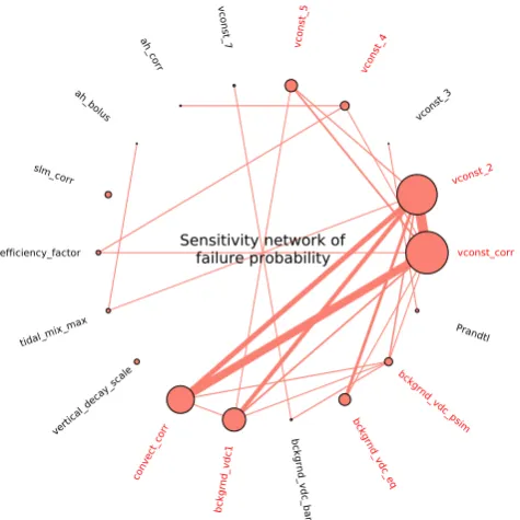
The technique has been extended to include higher order effects (e.g., using edgeij k for 3rd-order terms), but this is not needed for the current application. Important parameters on the resulting network graph are represented by nodes that are large or make significant connections to other nodes.

Figure 10 displays the network graph for the variance de-composition of log µc. Based on node size and

connec-tivity, the graph indicates that 8 out of the 18 parameters are the main drivers of the simulation failures (see param-eters labeled in red in the graph). These eight paramparam-eters account for about 95 % of the variance of log µc, as

quan-tified using Eq. (18). Of these,vconst corr,vconst 2,

convect corr, andbckgrnd vdc1stand out distinctly as the top four parameters in the graph. Recall that the same four parameters are described in Sect. 3 and displayed in Figs. 1 and 2. The top four parameters have the largest overall and most heavily connected nodes in the graph, and they collectively account for about 88 % of the variance of log µc. The strong connections indicate that the

(12)

Table 4. Polynomial chaos expansion of failure probability.

Expansion Leading terms∗

ξi

logµc≈ −4.347+4.049ξ1+3.400ξ2+2.267ξ13−1.980ξ14−1.393ξ16−1.253ξ5−

1.143ξ4−1.007ξ17−0.885ξ2ξ1−0.796ξ13ξ1−0.739ξ6−0.637ξ13ξ2−0.610ξ9+

0.578 ξ14 ξ2+0.480 ξ16 ξ2−0.471 ξ15−0.414 ξ12+0.382 ξ5 ξ1+0.372 ξ14 ξ1+

0.351ξ17ξ2+0.320ξ2ξ5+0.320ξ₈2+. . .

Pn(ξi)

logµc≈ −2.609+1.628P1(ξ1)+1.546P1(ξ2)+1.061P1(ξ13)−0.895P1(ξ14)−

0.475P1(ξ5)−0.455P1(ξ16)−0.338P1(ξ4)−0.311P1(ξ17)−0.245P1(ξ9)−

0.221P1(ξ1)P1(ξ2)−0.199P1(ξ1)P1(ξ13)+0.196P1(ξ12)+0.174P1(ξ10)+0.164P1(ξ11)−

0.159P1(ξ2)P1(ξ13)+0.145P1(ξ2)P1(ξ14)+0.133P1(ξ18)+0.120P1(ξ2)P1(ξ16)+

0.096P1(ξ1)P1(ξ5)+0.093P1(ξ1)P1(ξ14)+0.088P1(ξ2)P1(ξ17)−0.082P1(ξ6)+. . . ∗_{Leading terms are based on the magnitude of the absolute value of the coefficients of the polynomial chaos expansion. Refer to Table 1 for}

the parameter labels that correspond to the numbers. Discussion

P

ap

er

|

Discussion

P

ap

er

|

Discussion

P

ap

er

|

Di

scuss

ion

P

ap

er

|

vconst_corr vconst_2 vconst_3 vconst_4

vconst_5

vconst_7

ah_corr

ah_bolus

slm_corr

efficiency_factor

tidal_mix_max

vertical_decay_scale

convect_corr

bckgrnd_vdc1

bckgrnd_vdc_ban bckgrnd_vdc_eq

bckgrnd_vdc_psim Prandtl

Sensitivity network of

failure probability

Fig. 10.Sensitivity of the probability of simulation failure to climate model parameters is shown using a network graph. Node size and connector thickness are proportional to sensitivity contributions from individual parameters and pairs of parameters, respectively. The eight parameters labeled in red are the main causes of simulation failures.

39

Fig. 10. Sensitivity of the probability of simulation failure to cli-mate model parameters is shown using a network graph. Node size and connector thickness are proportional to sensitivity contributions from individual parameters and pairs of parameters, respectively. The eight parameters labeled in red are the main causes of simula-tion failures.

top four parameters. The direction of the dependence is de-termined by inspecting the signs of the corresponding coef-ficients in the polynomial chaos expansion (i.e., forξ1,ξ2,

ξ13, andξ14). Referring to Table 4, the failure probability

in-creases for increasing values ofvconst corr,vconst 2, andconvect corr, and increases for decreasing values of

bckgrnd vdc1, which is in accordance with the results in Figs. 1 and 2.

The variance decomposition therefore validates the de-scriptive relationships given in Sect. 3. However, it also

extends the failure analysis in important ways. Equation (18) quantitatively ranks the effects of the parameters on the sim-ulation failures, which provides a way to prioritize efforts to improve the model. This type of ranking cannot be easily ob-tained using just the scatterplots in Figs. 1 and 2. Moreover, the scatterplots show the correlations between the parameter values and simulation failures, but the one and two dimen-sional projections are not sufficient for separating the over-lappingCfandCs classes. Figure 10, on the other hand, very

clearly shows that four or more parameter dimensions are re-quired to explain and separate the simulation failures from the successes.

6 Summary and conclusions

(13)

models. The climate ensemble failure dataset used for all of the analysis presented in this manuscript is being made avail-able for public download at three sites (Bache and Lichman, 2013; MLdata.org, 2013; Lawrence Livermore National Lab-oratory Green Data Oasis, 2013).

Acknowledgements. Computing support for this work came from the Lawrence Livermore National Laboratory (LLNL) Institutional Computing Grand Challenge program. We thank G. Danabasoglu, M. Jochum, and R. Tokmakian for recommending the ocean model parameters and their uncertainty ranges. This work was performed under the auspices of the US Department of Energy by Lawrence Livermore National Laboratory under Contract DE-AC52-07NA27344, was funded by LLNL’s Uncertainty Quantification Strategic Initiative Laboratory Directed Research and Development Project under tracking code 10-SI-013, and is released under UCRL number LLNL-JRNL-608873. D. D. L. also received support from the DOE Office of Science through the Sci-entific Discovery Through Advanced Computing (SciDAC) project on Multiscale Methods for Accurate, Efficient, and Scale-Aware Models of the Earth System.

Edited by: J. Annan

References

Annan, J. D., Hargreaves, J. C., Edwards, N. R., and Marsh, R.: Parameter estimation in an intermediate complexity earth system model using an ensemble Kalman filter, Ocean Model., 8, 135– 154, doi:10.1016/j.ocemod.2003.12.004, 2005.

Arlot, S. and Celisse, A.: A survey of cross-validation procedures for model selection, Statistics Surveys, 4, 40–79, 2010. Bache, K. and Lichman, M.: UCI Machine Learning

Repos-itory, available at: http://archive.ics.uci.edu/ml (last access: 30 May 2013), archived on 12 September 2012: http://www. webcitation.org/6AcuZgrsy, 2013.

Bishop, C. M.: Pattern Recognition and Machine Learning, Infor-mation Science and Statistics, 1st Edn., Springer, 2007. Breiman, L.: Bagging predictors, Mach. Learn., 24, 123–140, 1996. Breiman, L.: Random forests, Mach. Learn., 45, 5–32, 2001. Breiman, L., Friedman, J. H., Olshen, R. A., and Stone, P. J.:

Classi-fication and Regression Trees, 1st Edn., Chapman and Hall/CRC, 1984.

Burges, C. J. C.: A tutorial on support vector machines for pattern recognition, Data Min. Knowl. Discov., 2, 121–167, 1998. CCSM4: The Community Climate System Model, Version 4,

avail-able at: http://www.cesm.ucar.edu/models/ccsm4.0/ (last access: 22 January 2013), archived on 21 July 2010: http://www. webcitation.org/5rOj1F8rL, 2012.

Chang, C. C. and Lin, C. J.: LIBSVM: A library for support vector machines, ACM Trans. Intell. Syst. Technol., 2, 27, doi:10.1145/1961189.1961199, 2011.

Clune, T. and Rood, R.: Software testing and verification in climate model development, IEEE Software, 28, 49–55, 2011.

Cortes, C. and Vapnik, V.: Support-vector networks, Mach. Learn., 20, 273–297, 1995.

Danabasoglu, G., Bates, S., Briegleb, B., Jayne, S., Jochum, M., Large, W., Peacock, S., and Yeager, S.: The CCSM4 ocean com-ponent, J. Climate, 25, 1361–1389, 2012.

Dietterich, T. G.: Ensemble methods in machine learning, in: Mul-tiple Classifier Systems, Lecture Notes in Computer Science, Springer Berlin Heidelberg, 1857, 1–15, 2000.

D’Silva, V., Kroening, D., and Weissenbacher, G.: A survey of automated techniques for formal software verification, IEEE T. Comput.-Aid. D., 27, 1165–1178, 2008.

Easterbrook, S. M.: Climate change: a grand software challenge, in: FoSER, edited by: Roman, G.-C. and Sullivan, K. J., 99–104, ACM, 2010.

Easterbrook, S. M.: Do Over or Make Do? Climate Models as a Software Development Challenge, 2012 Fall Meeting Ab-stracts, IN14B-01, AGU, San Francisco, Calif., 3–7 December, 2012.

Easterbrook, S. M. and Johns, T. C.: Engineering the software for understanding climate change, Comput. Sci. Eng., 11, 65–74, 2009.

Easterbrook, S. M., Edwards, P. N., Balaji, V., and Budich, R.: Guest editors’ introduction: climate change – science and soft-ware, IEEE Softsoft-ware, 28, 32–35, 2011.

Edwards, N. R., Cameron, D., and Rougier, J.: Precalibrating an in-termediate complexity climate model, Clim. Dynam., 37, 1469– 1482, doi:10.1007/s00382-010-0921-0, 2011.

Farrell, P. E., Piggott, M. D., Gorman, G. J., Ham, D. A., Wil-son, C. R., and Bond, T. M.: Automated continuous verifica-tion for numerical simulaverifica-tion, Geosci. Model Dev., 4, 435–449, doi:10.5194/gmd-4-435-2011, 2011.

Fawcett, T.: An introduction to ROC analysis, Pattern Recogn. Lett., 27, 861–874, 2006.

Forrester, A. I. J., Sobester, A., and Keane, A. J.: Engineering De-sign via Surrogate Modelling – A Practical Guide, Wiley, 2008. Fox-Kemper, B., Ferrari, R., and Hallberg, R.: Parameterization

of mixed layer eddies, Part I: Theory and diagnosis, J. Phys. Oceanogr., 38, 1145–1165, 2008.

Gent, P. R. and McWilliams, J. C.: Isopycnal mixing in ocean cir-culation models, J. Phys. Oceanogr., 20, 150–155, 1990. Gent, P. R., Danabasoglu, G., Donner, L. J., Holland, M. M.,

Hunke, E. C., Jayne, S. R., Lawrence, D. M., Neale, R. B., Rasch, P. J., Vertenstein, M., Worley, P. H., Yang, Z.-L., and Zhang, M.: The Community Climate System Model Version 4, J. Climate, 24, 4973–4991, 2011.

Griffies, S.: Fundamentals of Ocean Climate Models, Princeton University Press, 2004.

Helton, J. C. and Davis, F. J.: Latin hypercube sampling and the propagation of uncertainty in analyses of complex systems, Re-liab. Eng. Syst. Safe., 81, 23–69, 2003.

Helton, J., Johnson, J., Sallaberry, C., and Storlie, C.: Survey of sampling-based methods for uncertainty and sensitivity analysis, Reliab. Eng. Syst. Safe., 91, 1175–1209, 2006.

Hosmer, D. W. and Lemeshow, S.: Applied Logistic Regression, 2nd Edn., Wiley-Interscience, 2000.

Jackson, C., Sen, M., Huerta, G., Deng, Y., and Bowman, K.: Error reduction and convergence in climate prediction, J. Climate, 21, 6698–6709, 2008.

(14)

Jochum, M., Danabasoglu, G., Holland, M., Kwon, Y.-O., and Large, W. G.: Ocean viscosity and climate, J. Geophys. Res., 113, C06017, doi:10.1029/2007JC004515, 2008.

Kotsiantis, S. B.: Supervised Machine Learning: a Review of Clas-sification Techniques, in: Proceedings of the 2007 conference on Emerging Artificial Intelligence Applications in Computer Engi-neering: Real Word AI Systems with Applications in eHealth, HCI, Information Retrieval and Pervasive Technologies, IOS Press, Amsterdam, The Netherlands, The Netherlands, 3–24, 2007.

Large, W. and Yeager, S.: The global climatology of an interannu-ally varying air–sea flux data set, Clim. Dynam., 33, 341–364, 2009.

Large, W. G., McWilliams, J. C., and Doney, S. C.: Oceanic vertical mixing: A review and a model with a nonlocal boundary layer parameterization, Rev. Geophys., 32, 363–403, 1994.

Large, W. G., Danabasoglu, G., McWilliams, J. C., Gent, P. R., and Bryan, F. O.: Equatorial circulation of a global ocean climate model with anisotropic horizontal viscosity, J. Phys. Oceanogr., 31, 518–536, 2001.

Lawrence Livermore National Laboratory Green Data Oasis, avail-able through anonymous ftp at: ftp://gdo148.ucllnl.org/pub/ (last access: 24 June 2013), 2013.

Lucas, D. D. and Prinn, R. G.: Parametric sensitivity and uncer-tainty analysis of dimethylsulfide oxidation in the clear-sky re-mote marine boundary layer, Atmos. Chem. Phys., 5, 1505– 1525, doi:10.5194/acp-5-1505-2005, 2005.

Marzban, C.: The ROC curve and the area under it as performance measures, Weather Forecast., 124, 1106–1113, 2004.

McKay, M. D., Beckman, R. J., and Conover, W. J.: A compari-son of three methods for selecting values of input variables in the analysis of output from a computer code, Technometrics, 21, 239–245, 1979.

MLdata.org: Machine learning data set repository, avail-able at: http://mldata.org/repository/data/viewslug/ climate-model-simulation-crashes/ (last access: 24 June 2013), archived on 24 June 2013: http://www.webcitation.org/ 6HcrKQ4Lk, 2013.

Murphy, J., Sexton, D., Barnett, D., Jones, G., Webb, M., Collins, M., and Stainforth, D.: Quantification of modelling un-certainties in a large ensemble of climate change simulations, Nature, 430, 768–772, 2004.

National Research Council Report: Assessing the Reliability of Complex Models: Mathematical and Statistical Foundations of Verification, Validation, and Uncertainty Quantification, The Na-tional Academies Press, 2012.

Pipitone, J. and Easterbrook, S.: Assessing climate model software quality: a defect density analysis of three models, Geosci. Model Dev., 5, 1009–1022, doi:10.5194/gmd-5-1009-2012, 2012. Platt, J. C.: Probabilistic outputs for support vector machines and

comparisons to regularized likelihood methods, in: Advances in Large Margin Classifiers, MIT Press, 61–74, 1999.

Prati, R. C., Batista, G. E. A. P. A., and Monard, M. C.: Class imbalances versus class overlapping: an analysis of a learning system behavior, in: MICAI, edited by: Monroy, R., Arroyo-Figueroa, G., Sucar, L. E., and Azuela, J. H. S., Lecture Notes in Computer Science, vol. 2972, Springer, 312–321, 2004. Randall, D., Wood, R., Bony, S., Colman, R., Fichefet, T., Fyfe, J.,

Kattsov, V., Pitman, A., Shukla, J., Srinivasan, J., Stouffer, R.,

Sumi, A., and Taylor, K.: Climate Models and Their Evaluation, in: Climate Change 2007: The Physical Science Basis, Contri-bution of Working Group I to the Fourth Assessment Report of the Intergovernmental Panel on Climate Change, edited by: Solomon, S., Qin, D., Manning, M., Chen, Z., Marquis, M., Av-eryt, K. B., Tignor, M., and Miller, H. L., Cambridge University Press, 2007.

Rugaber, S., Dunlap, R., Mark, L., and Ansari, S.: Managing soft-ware complexity and variability in coupled climate models, IEEE Software, 28, 43–48, 2011.

Saltelli, A., Chan, K., and Scott, E. M.: Sensitivity Analysis, Wiley, 2000.

Sanderson, B.: A multimodel study of parametric uncertainty in pre-dictions of climate response to rising greenhouse gas concentra-tions, J. Climate, 24, 1362–1377, 2011.

Shiogama, H., Watanabe, M., Yoshimori, M., Yokohata, T., Ogura, T., Annan, J. D., Hargreaves, J. C., Abe, M., Kamae, Y., O’ishi, R., Nobui, R., Emori, S., Nozawa, T., Abe-Ouchi, A., and Kimoto, M.: Perturbed physics ensemble using the MIROC5 coupled atmosphere-ocean GCM without flux corrections: exper-imental design and results, Clim. Dynam., 39, 3041–3056, 2012. Smith, R., Jones, P., Briegleb, B., Bryan, F., Danabasoglu, G., Dennis, J., Dukowicz, J., Eden, C., Fox-Kemper, B., Gent, P., Hecht, M., Jayne, S., Jochum, M., Large, W., Lindsay, K., Mal-trud, M., Norton, N., Peacock, S., Vertenstein, M., and Yeager, S.: The Parallel Ocean Program (POP) reference manual, ocean component of the Community Climate System Model (CCSM), Tech. Rep. LAUR-10-01853, Los Alamos National Laboratory, 141 pp., 2010.

Smith, R. D. and McWilliams, J. C.: Anisotropic horizontal viscos-ity for ocean models, Ocean Model., 5, 129–156, 2003. Sobol, I. M.: Global sensitivity indices for nonlinear mathematical

models and their Monte Carlo estimates, Math. Comput. Simu-lat., 55, 271–280, 2001.

Stainforth, D., Aina, T., Christensen, C., Collins, M., Faull, N., Frame, D. J., Kettleborough, J. A., Knight, S., Martin, A., Mur-phy, J. M., Piani, C., Sexton, D., Smith, L. A., Spicer, R. A., Thorpe, A. J., and Allen, M. R.: Uncertainty in predictions of the climate response to rising levels of greenhouse gases, Nature, 433, 403–406, 2005.

Stein, M.: Large sample properties of simulations using Latin hy-percube sampling, Technometrics, 29, 143–151, 1987.

Stensrud, D. J.: Parameterization Schemes: Keys to Understand-ing Numerical Weather Prediction Models, Cambridge Univer-sity Press, 2009.

Sudret, B.: Global sensitivity analysis using polynomial chaos ex-pansions, Reliab. Eng. Syst. Safe., 93, 964–979, 2008.

Swets, J. A.: Measuring the accuracy of diagnostic systems, Sci-ence, 240, 1285–1293, 1988.

Tannahill, J., Lucas, D. D., Domyancic, D., Brandon, S., and Klein, R.: Data intensive uncertainty quantification: Appli-cations to climate modeling, in: Poster Presented at Super Computing 11, November 12–18, Seattle, Washington, USA, doi:10.1145/2148600.2148610, 2011.

Tatang, M., Pan, W., Prinn, R., and McRae, G.: An efficient method for parametric uncertainty analysis of numerical geophysical models, J. Geophys. Res., 102, 21925–21932, 1997.