www.geosci-model-dev.net/9/3447/2016/ doi:10.5194/gmd-9-3447-2016
© Author(s) 2016. CC Attribution 3.0 License.
The Radiative Forcing Model Intercomparison Project (RFMIP):
experimental protocol for CMIP6
Robert Pincus1,2, Piers M. Forster3, and Bjorn Stevens4
1Cooperative Institute for Research in Environmental Sciences, University of Colorado, Boulder, CO 80309, USA 2NOAA Earth System Research Lab, Physical Sciences Division, Boulder, CO 80305, USA
3Institute for Climate and Atmospheric Science, School of Earth and Environment, University of Leeds, Leeds, UK 4Max Planck Institute for Meteorology, Hamburg 20146, Germany
Correspondence to:Robert Pincus ([email protected])
Received: 12 April 2016 – Published in Geosci. Model Dev. Discuss.: 19 May 2016
Revised: 7 September 2016 – Accepted: 16 September 2016 – Published: 27 September 2016
Abstract. The phrasing of the first of three questions mo-tivating CMIP6 – “How does the Earth system respond to forcing?” – suggests that forcing is always well-known, yet the radiative forcing to which this question refers has his-torically been uncertain in coordinated experiments even as understanding of how best to infer radiative forcing has evolved. The Radiative Forcing Model Intercomparison Project (RFMIP) endorsed by CMIP6 seeks to provide a foundation for answering the question through three related activities: (i) accurate characterization of the effective radia-tive forcing relaradia-tive to a near-preindustrial baseline and care-ful diagnosis of the components of this forcing; (ii) assess-ment of the absolute accuracy of clear-sky radiative trans-fer parameterizations against retrans-ference models on the global scales relevant for climate modeling; and (iii) identification of robust model responses to tightly specified aerosol radia-tive forcing from 1850 to present.
Complete characterization of effective radiative forcing can be accomplished with 180 years (Tier 1) of atmosphere-only simulation using a sea-surface temperature and sea ice concentration climatology derived from the host model’s preindustrial control simulation. Assessment of parameter-ization error requires trivial amounts of computation but the development of small amounts of infrastructure: new, spectrally detailed diagnostic output requested as two snap-shots at present-day and preindustrial conditions, and results from the model’s radiation code applied to specified atmo-spheric conditions. The search for robust responses to aerosol changes relies on the CMIP6 specification of anthropogenic aerosol properties; models using this specification can
con-tribute to RFMIP with no additional simulation, while those using a full aerosol model are requested to perform at least one and up to four 165-year coupled ocean–atmosphere sim-ulations at Tier 1.
1 Evolving understanding of radiative forcing
Perturbations to the chemical or physical state of the climate system, including those caused by anthropogenic activities, can induce a radiative perturbation loosely called a radia-tive forcing. Projections of future changes involve estimating the magnitude of future radiative forcing and the strength of climate system’s response to that forcing. If the system’s re-sponse can be adequately described by a single temperature
T (normally the global-mean surface temperature), then ra-diative forcingF is related to the top-of-atmosphere energy imbalanceN(or equivalently, global ocean heat uptake) and the temperature change1T as
F =N+α1T , (1)
where the constant of proportionality between temperature and radiative responseαis the climate feedback parameter.
underlies the question “How does the Earth system respond to forcing?” – one of the central questions motivating the sixth phase of the CMIP (CMIP6; see Eyring et al., 2016). The formulation of this question presumes that the forcing to which the Earth system, or a model representation of the sys-tem, is subject is well-known. But this is not true in practice: models participating in exercises like CMIP are subject to surprisingly large differences in radiative forcing (Andrews et al., 2012; Forster et al., 2013; Chung and Soden, 2015) even when the perturbations applied to the physical system are the same. The radiative forcing to which the Earth it-self has been subject is also relatively uncertain (e.g., Skeie et al., 2011). Even the concept of radiative forcing continues to evolve (Sherwood et al., 2015) in a search for informa-tive measures and precise methods for diagnosis. To answer questions about how the Earth system responds to forcing it is first necessary both to understand the nature of radiative forcing and to quantify the forcing experienced by individual models.
Some differences arise because individual models produce a range of radiative changes for the same physical pertur-bation. Specifying atmospheric composition changes, as has been common in previous phases of CMIP, does not uniquely determine even the instantaneous change in radiative fluxes at the top of the atmosphere (the “instantaneous radiative forcing” or IRF, in the language of Myhre et al., 2013). This is partly because extinction by gases depends on the distribu-tions of temperature and humidity, which vary across models, and partly because computationally efficient parameteriza-tions for radiative transfer will differ to varying degrees with respect to reference models. This non-uniqueness is most rel-evant to radiative forcing by greenhouse gases, changes in which are responsible for the largest forcing since preindus-trial times (Myhre et al., 2013).
Differences also arise because models make different choices with respect to important but uncertain or loosely specified physical perturbations, especially aerosols (Shin-dell et al., 2013), which, after greenhouse gases, are thought to be responsible for the second largest source of anthro-pogenic radiative perturbations. In the previous phase of CMIP the breadth of direct aerosol impacts on top-of-atmosphere radiation was larger than that due to greenhouses gases even as the signal was∼3 times smaller (e.g., Myhre et al., 2013, their Fig. 8.16).
Equation (1) is a diagnostic framework, useful in inter-preting observations and comprehensive models of the cli-mate system. Experience with models (in which all terms can be determined precisely) suggests that IRF is not, in prac-tice, related very closely to changes in surface temperature, a point highlighted by Hansen et al. (1997) but well-known for even longer. Far more useful in Eq. (1) is theeffective ra-diative forcing(ERF) that accounts foradjustments, the com-ponent of climate response that does not depend on global-mean surface temperature (Sherwood et al., 2015). Many such adjustments, for example the reduction in oceanic
sub-tropical boundary layer cloudiness due to increased down-welling longwave radiation from increased CO2, occur much more rapidly than the timescale for warming (e.g., Kamae and Watanabe, 2012) leading to the terminology “rapid ad-justments”. Rapid adjustments are generalizations of (and re-place) the stratospheric adjustment (Hansen et al., 1997) that has historically been used to account for the impact of rapid stratospheric equilibration on top-of-atmosphere radiation fluxes. Accurate diagnosis of ERF requires custom model in-tegrations, either using linear regression to diagnoseF and
α(assumed constant) in Eq. (1) from temporal variations in
N and1T following abruptly applied changes in composi-tion (Gregory et al., 2004), or by approximately suppressing
1T by fixing sea surface temperatures (SSTs) and inferring effective radiative forcing from N following Hansen et al. (2005) and Rotstayn and Penner (2001). The diagnosis of ERF from such simulations is simplified, however, because ERF is diagnosed from changes in top-of-atmosphere radi-ation. Unlike the radiative perturbation arising from a com-position change, ERF depends on the fullness of system re-sponse, so its calculation is no longer an exercise in pure ra-diative transfer.
Better estimates of effective radiative forcing will refine understanding of how the Earth system responds to forc-ing, but the potentially knotty relationships between radia-tive forcing and response suggest value in subjecting models to ERFs that are as similar as possible. In signal processing it is common, when looking for a signal amidst a noisy back-ground, to reduce the noise as close to the source as possi-ble. In the context of ERF the largest source of variability is the treatment of atmospheric aerosol. The Radiative Forcing Model Intercomparison Project (RFMIP) therefore includes coupled atmosphere–ocean simulations in which aerosol ef-fective radiative forcing over the historical period is pre-scribed as much as possible, by analogy to protocols in which greenhouse gas concentrations over time are similarly spec-ified. This is not to diminish the true uncertainty in histori-cal concentration of anthropogenic aerosols but to ascertain what model responses robustly arise from a plausible histor-ical aerosol radiative forcing.
RFMIP seeks to provide a foundation for answering one of the guiding questions of CMIP6, namely “how does the Earth system respond to forcing?” This will be accomplished by
1. accurately characterizing the effective radiative forcing relative to a near-preindustrial baseline and understand-ing the components of this forcunderstand-ing,
2. assessing the absolute accuracy of clear-sky radiative transfer parameterizations on the global scales relevant for climate modeling, and
This paper describes each of these efforts in greater detail, in-cluding the contributions requested from participating mod-eling centers, reference calculations to be undertaken as part of RFMIP, and planned analyses. The simulations are sum-marized in tables below.
RFMIP follows CMIP6 protocols so that “present day” is interpreted as the year 2014 and “greenhouse gases” re-fer to those specified by Meinshausen et al. (2016), i.e., CO2, CH4, N2O, and a long list of halocarbons. Ozone con-centrations are specified separately from greenhouse gases but in concert with aerosols. Here we provide brief sum-maries of requested output, but the definitive, detailed, and still-evolving specification is documented in the CMIP6 data request available at https://earthsystemcog.org/projects/wip/ CMIP6DataRequest.
2 Diagnosing effective radiative forcing
The concept of radiative forcing has evolved over time, as can be seen by comparing the discussions in Hansen et al. (1997) with those in Sherwood et al. (2015), which we follow here. Partly for this reason, and partly because the climate system response was considered the largest unknown, pre-vious iterations of CMIP have emphasized model response without careful characterization of effective radiative forc-ing. This omission has made it challenging to understand the degree to which differences in model response arise purely from different feedbacks. In the previous phase of CMIP, for example, models exhibited a wide range of global-mean temperature changes over the historical period (1860–2005 for CMIP5). These models were driven by the same con-centration or emission changes, but for the reasons described above the same concentration time series applied to different models led to different temporal evolutions of ERF including rapid adjustments (Forster et al., 2013). The extent to which the varying responses in CMIP3 and CMIP5 historical simu-lations were due to differences in effective radiative forcing among models, as opposed to differences in feedbacks, re-mains unknown.
Limited understanding of ERF has severely hampered progress in key areas of physical climate science, includ-ing understandinclud-ing historical temporal and spatial variations in climate feedbacks (Armour et al., 2013; Rose et al., 2014; Andrews et al., 2015); attribution of aerosol and greenhouse gas signals from the historic record (Bindoff et al., 2013); di-agnosis of equilibrium climate sensitivity from observed en-ergy budget changes (Masters, 2013; Otto et al., 2013); diag-nosing transient climate response from historic trends (Gre-gory and Forster, 2008; Storelvmo et al., 2016); understand-ing the causes of global and regional precipitation trends (Richardson et al., 2016); and understanding of decadal vari-ations in surface temperature, including the recent “hiatus” in surface warming (Marotzke and Forster, 2015; Fyfe et al., 2016).
RFMIP will diagnose model ERF by suppressing re-sponse, i.e., specifying SST and sea ice concentrations (Hansen et al., 2005). The “fixed-SST” method has important advantages compared to regressions of top-of-atmosphere imbalance against surface temperature change (Gregory et al., 2004). The most important is better error character-istics (Forster et al., 2016): 30 years of simulation using only the atmospheric and land components of an Earth system model can diagnose global ERF to better than 0.05 W m−2 standard error, such that a 2×CO2effective radiative forc-ing of 3.7 W m−2is larger than its standard error over 70 % of the globe. Achieving similarly small errors from regres-sion requires ensembles of coupled model integrations and therefore many centuries of simulation. Using fixed SSTs also allows model groups to diagnose transient ERF while regressions are suitable only for diagnosing ERF from abrupt changes. Transient ERFs are of particular interest in histori-cal simulations.
2.1 Protocol: effective radiative forcing
The protocol for RFMIP fixed-SST integrations is to use a model-specific monthly averaged climatology of SST and sea ice based on the model’s preindustrial DECK integra-tion (Eyring et al., 2016). Applying a climatology limits vari-ability and improves the diagnoses of small ERF differences. The same climatology is to be used for all ERF integrations. We request that distributions from a monthly averaged cli-matology of SST and sea ice fractional coverage covering the annual cycle be generated from at least a 30-year seg-ment of a preindustrial control integration. These should be prescribed according to the AMIP protocols, whereby inter-polated daily data are generated preserving the prescribed monthly averaged fields. Because ERF is weakly dependent on background state (Forster et al., 2016) the exact choice of background SST and sea ice has little impact on the effec-tive radiaeffec-tive forcing estimated in the historic period and in future climates (see below). We hope that a simple approach will encourage modeling centers to participate.
Time-slice simulations (Table 1), in which forcing agents are held constant at present-day or 4×CO2values, provide estimates of present-day and 4×CO2ERF. Present-day esti-mates provide a direct comparison between the estiesti-mates of ERF in the model with other estimates, e.g., in assessment reports (Myhre et al., 2013). Estimates of ERF will also let us understand basic aspects of each model’s temperature and other climate responses in the historical and 4×CO2DECK simulations.
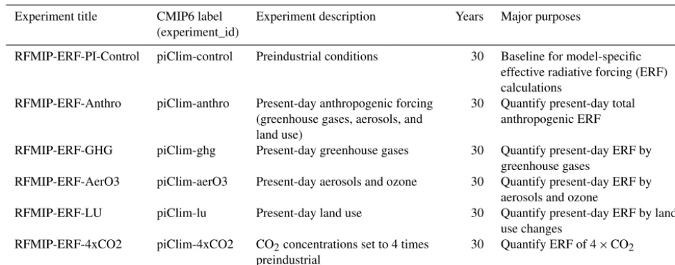
Table 1.Experiments for diagnosing effective radiative forcing at present day and under 4×CO2conditions. These are atmosphere-only integrations with interactive vegetation using sea-surface temperatures and sea ice concentrations fixed at model-specific preindustrial control climatology. All experiments are perturbations to RFMIP-ERF-PI-Cntrl and are requested at Tier 1.
Experiment title CMIP6 label Experiment description Years Major purposes (experiment_id)
RFMIP-ERF-PI-Control piClim-control Preindustrial conditions 30 Baseline for model-specific effective radiative forcing (ERF) calculations
RFMIP-ERF-Anthro piClim-anthro Present-day anthropogenic forcing (greenhouse gases, aerosols, and land use)
30 Quantify present-day total anthropogenic ERF
RFMIP-ERF-GHG piClim-ghg Present-day greenhouse gases 30 Quantify present-day ERF by greenhouse gases
RFMIP-ERF-AerO3 piClim-aerO3 Present-day aerosols and ozone 30 Quantify present-day ERF by aerosols and ozone
RFMIP-ERF-LU piClim-lu Present-day land use 30 Quantify present-day ERF by land use changes
RFMIP-ERF-4xCO2 piClim-4xCO2 CO2concentrations set to 4 times preindustrial
30 Quantify ERF of 4×CO2
Table 2.Experiments for diagnosing time-evolving effective radiative forcing. Three-member ensembles of atmosphere-only integrations interactive vegetation and using sea-surface temperatures and sea ice concentrations fixed at model-specific preindustrial control climatology. Forcing post-2015 uses a scenario consistent with DCPP and DAMIP (SSP2-4.5).
Experiment title CMIP6 label Experiment description Start End Major purposes (experiment_id)
RFMIP-ERF-HistAll piClim-histall Time-varying forcing from all agents
1850 2100 Diagnose transient ERF from all agents
RFMIP-ERF-HistNat piClim-histnat Time-varying ERF from volca-noes, solar (including spectral) variability
1850 2100 Diagnose transient natural ERF
RFMIP-ERF-HistGHG piClim-histghg Time-varying ERF by greenhouse gases
1850 2100 Diagnose transient ERF from greenhouse gases
RFMIP-ERF-HistAerO3 piClim-histaerO3 Time-varying ERF by aerosols 1850 2100 Diagnose transient ERF from aerosols
from the 30-year control simulation. These integrations will use the same prescribed preindustrial climatology of SST and sea ice as in the time-slice ERF experiments. AerChem-MIP employs a more complex method of prescribing SSTs and sea ice that allows for base climate changes through time. Offline tests found that such complexity was unnec-essary as ERF was only weakly dependent on the base state with small differences in the future confined to sea ice edges (Forster et al., 2016). Therefore RFMIP adopts the same base climatology in all experiments for ease of implemen-tation. Tests also found that the transient ERF fields suf-fer from year-to-year random noise, so 10-year averages of the three ensemble members are needed to quantify ERF to within 0.05 W m−2(Forster et al., 2016). The future scenario (SSP2.4.5) matches experimental protocols requested by the Decadal Climate Prediction Project (DCCMIP, Boer et al., 2016) and the Detection and Attribution Model
Intercom-parison Project (DAMIP, Gillett et al., 2016). The full ERF history from these simulations will give a much better un-derstanding of decadal variability in the models and will aid attribution studies.
Land-surface models including interactive vegetation, if available, should be applied as in other CMIP integrations. The main diagnostics are the top of atmosphere energy bud-get terms required to estimate ERF. Diagnostics of atmo-spheric state, including temperature, water vapor, cloud and aerosol information, are requested to allow for detailed di-agnosis of rapid adjustments. A few daily variables related to temperature and precipitation are requested in conjunc-tion with DAMIP to help distinguish direct effects of external forcing and air–sea interaction effects on historical changes in extreme indices (e.g., extreme precipitation).
partic-ipate in no other aspect of RFMIP. Knowing the present-day and 4×CO2ERF will enable modeling centers to understand why their DECK and historical simulations differ from those performed by other models. Having all modeling centers per-form these is important to understand outliers in the multi-model ensemble, allowing us to probe whether outliers are caused by radiative forcing-related or feedback-related pro-cesses. Further, the transient simulations in Table 2 are im-portant for understanding model decadal variability and tran-sient variations in climate feedbacks. This will benefit both decadal projections and attribution.
2.2 Planned analyses: effective radiative forcing
Global and regional effective radiative forcing will be diag-nosed for each model participating in RFMIP by differenc-ing top-of-atmosphere radiative fluxes from the experiment with those from the preindustrial control simulation. RFMIP will characterize present day, historical and future ERF for the main radiative forcing groups (CO2, all anthropogenic forcings, land use, and aerosol and ozone changes taken together; see Tables 1 and 2). Aerosol and ozone changes are investigated together to allow participation from both concentration-driven and emission-driven models, as emis-sions of NOx, for example, can drive both ozone and aerosol
changes. The complimentary Aerosols Chemistry Model In-tercomparison Project (AerChemMIP, Collins et al., 2016) ERF simulations adopt the same calculation methodology as RFMIP for Tier 1 experiments. AerChemMIP targets interac-tive chemistry models and extends RFMIP to allow the com-munity to further decompose present-day aerosol and non-CO2ERFs into a more finely delineated set of ERFs for dif-ferent sets of precursor emissions.
Regional patterns of ERF will be compared across the models. This will aid the understanding of regional differ-ences in climate response including an investigation of spa-tial variation in climate feedbacks.
The rapid adjustment component of effective radiative forcing will also be investigated. Rapid adjustments associ-ated with aerosol–cloud interaction are the major contribu-tor to the negative aerosol ERF, and quantifying these ef-fects has been a focus of much previous work (Boucher et al., 2013). Rapid adjustments are also important for many forc-ing agents includforc-ing CO2(Sherwood et al., 2015). RFMIP re-quests joint histograms of cloud optical thickness and cloud top pressure from the “ISCCP simulator” (Klein and Jakob, 1999; Webb et al., 2001), part of the CFMIP Observation Simulator Package (Bodas-Salcedo et al., 2011) providing specialized diagnostics for the Cloud Feedback Model Inter-comparison Project (CFMIP, see Webb et al., 2016). These will be used to estimate rapid adjustments by clouds using ra-diative kernels (Zelinka et al., 2012, 2014) that map changes in cloud properties into top-of-atmosphere radiative flux per-turbations. Where these diagnostics are not available the ap-proximate partial radiative perturbation methodology of
Tay-lor et al. (2007) will be applied to clear-sky and all-sky com-ponents of shortwave (SW) radiative fluxes, to estimate the rapid adjustments due to cloud changes. Non-cloud radiative kernels (Soden et al., 2008) will also be applied to standard diagnostics of water vapor and temperature to estimate IRF as well as stratospheric and tropospheric adjustments (Zhang and Huang, 2014; Chung and Soden, 2015).
These analyses will comprehensively characterize ERF in each model participating in RFMIP. Radiative kernel diag-nostics will enable us to develop understanding of rapid ad-justment processes. We will test the kernel approach by com-paring pre-adjustment radiative perturbations at the top-of-atmosphere estimated from radiative kernels with the best es-timate of those perturbations from the line-by-line radiative transfer models according to the experimental design out-lined in Sect. 3. In the same spirit we are interested in com-paring radiative perturbations and cloud adjustments esti-mated from radiative kernels with those explicitly calculated in models employing the “triple radiation call” approach of Ghan (2013) to diagnose instantaneous radiative forcing and cloud adjustments. As this method is time-consuming and not implemented by all models, we do not include this re-quest as part of the protocol but models implementing triple radiation calls are encouraged to contact us.
3 Assessing parameterization error in clear-sky radiative forcing
One of the causes for model differences in effective radiative forcing for the same physical perturbation is error in radiative transfer parameterizations. This is somewhat surprising: ra-diative transfer is unique among the processes parameterized in atmospheric models because there is so little fundamen-tal uncertainty. Line-by-line models can map atmospheric conditions and gas concentrations to extinction with very high accuracy and at very high spectral resolution. Transport algorithms, given enough computing resources, can com-pute fluxes to a precision limited primarily by uncertainty in inputs. But this deep knowledge is not completely repre-sented in climate models. Parameterizations strike a practical compromise between accuracy and computational cost and might be expected to have some error even under the best of circumstances. More subtly, parameterizations require so much effort to develop and maintain that they can lag behind current spectroscopic knowledge, especially for solar radia-tion where new absorpradia-tion features continue to be identified (Rothman et al., 2013). These errors have been apparent in previous assessments of radiative transfer parameterizations for both gaseous absorption (Ellingson and Fouquart, 1991; Collins et al., 2006; Oreopoulos et al., 2012; Pincus et al., 2015) and aerosols (Randles et al., 2013).
different approaches but will both highlight global- and regional-mean errors.
Despite the important roles of clouds in modulating ef-fective radiative forcing, RFMIP focuses on parameteriza-tion error in cloud-free skies. This is partly because errors in clear skies are always present and may affect, e.g., surface fluxes even when the top-of-atmosphere impact is masked by clouds, and partly because inter-model differences in the spatial and temporal distribution of clouds, which arise from complicated interactions between parameterizations and cir-culation, are likely to have a much larger impact on estimates of radiative forcing than are parameterization errors. 3.1 Protocol: parameterization error
Assessments of radiative transfer parameterizations rely on computationally expensive reference models. This has his-torically meant that only a few atmospheric conditions are considered, making it difficult to infer the error in global-mean radiative perturbations (Pincus et al., 2015) or the flux pairs which underlie them. The narrow range of conditions has also obscured some crucial differences between param-eterizations, most notably the widely varying sensitivity of shortwave absorption to water vapor that causes much of the variability in hydrologic sensitivity among climate models (Fildier and Collins, 2015; DeAngelis et al., 2015).
3.1.1 Assessing accuracy in the treatment of greenhouse gases
RFMIP is developing a compact (roughly 100) sample of at-mospheric conditions (profiles of pressure, temperature, hu-midity, greenhouse gas concentrations, surface properties) and radiative transfer boundary conditions (solar geometry and solar constant) that, when weighted appropriately, can be used to estimate time-averaged global-mean fluxes (sampling approaches are common in remote sensing problems; see for example Garand et al., 2001). Present-day atmospheric and surface conditions are sampled from reanalysis while green-house gas concentrations follow the CMIP6 protocol, using 2014 values provided by Meinshausen et al. (2016). Aerosols are not included. Perturbations to these states allow for the calculation of IRF as the difference in flux between a per-turbed state and present-day conditions and concentrations. Some perturbed states (see Table 3) represent changes in con-ditions tied to CMIP DECK or historical simulations. The more idealized perturbations described in Table 4 are aimed at exposing model errors with global impacts, especially in present-day radiative forcing by specific greenhouse gases, while three experiments in the table assess radiative transfer performance in conditions far from present day. This set of conditions will be distributed on the Earth System Grid as a single file.
The sample is constructed to minimize the sampling er-ror in annual-mean, present-day, clear-sky, aerosol-free
ra-diative perturbation by greenhouse gases (i.e., the difference in top-of-atmosphere fluxes using present-day and preindus-trial gas concentrations). The sampling error, even with as few as 50 distinct conditions, is several orders of magnitude smaller than the flux perturbation itself. Sampling errors for other composition changes are larger but still small relative to the change in flux. Further details on the selection of these columns will be reported separately.
Modeling centers are asked to compute broadband (spec-trally integrated) fluxes for the full range of conditions and all perturbations using offline versions of their radiative trans-fer parameterizations (or using any workflow that computes fluxes as the host model does using precisely the specified conditions). Modeling centers are asked to use the vertical grid provided and to omit aerosols. The representation of greenhouse gases, and particularly the choice of using a sub-set of gases or one of the equivalent concentrations provided by Meinshausen et al. (2016), should follow that used in other integrations made for CMIP6 and related activities.
Results from one or more reference models will also be made available on the Earth System Grid, as discussed in Sect. 3.2.
3.1.2 Assessing accuracy in the treatment of aerosols
The assessment of aerosol instantaneous clear-sky (direct) ra-diative perturbations seeks to determine parameterization er-ror “in the wild”, i.e., under climatological conditions spe-cific to each model. The effort is diagnostic: we request from modeling centers climate model estimates of clear-sky IRF due to aerosols and the detailed optical properties nec-essary to reconstruct this estimate, including instantaneous four-dimensional fields of spectrally resolved surface albedo, aerosol extinction, single-scattering albedo, and asymmetry parameter on the models native atmospheric grid and using the native spectral discretization. The request is limited to solar radiation, and to a single day in the preindustrial and present-day epoch taken from the model’s CMIP6 historical simulations. Participation involves no additional simulation but does require producing outputs new to CMIP that include a spectral dimension.
3.2 Planned analyses and supporting calculations: parameterization error
Table 3.Sets of atmospheric conditions to be supplied by RFMIP for assessing parameterization error in clear-sky top-of-atmosphere flux changes. The entire set of conditions is described as CMIP experiment RFMIP-IRF with CMIP6 label (experiment_id) rad-irf.
Atmospheric conditions Gas concentrations Major purpose Relevant experiment
Present-day Present-day Baseline
Present-day Preindustrial Present-day radiative forcing Historical Present-day 4×preindustrial CO2 Radiative forcing from 4×CO2 abrupt4xCO2 Present-day “Future” Radiative forcing in future conditions RCP8.5 at 2100
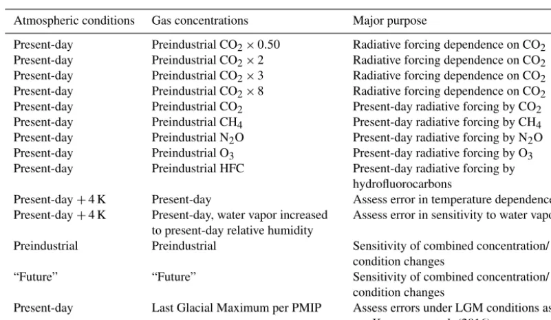
Table 4.Sets of atmospheric conditions to be supplied by RFMIP for assessing radiative forcing by specific agents and probing sources of parameterization error. The entire set of conditions is described as CMIP experiment RFMIP-IRF with CMIP6 Label (experiment_id) rad-irf.
Atmospheric conditions Gas concentrations Major purpose
Present-day Preindustrial CO2×0.50 Radiative forcing dependence on CO2 Present-day Preindustrial CO2×2 Radiative forcing dependence on CO2 Present-day Preindustrial CO2×3 Radiative forcing dependence on CO2 Present-day Preindustrial CO2×8 Radiative forcing dependence on CO2 Present-day Preindustrial CO2 Present-day radiative forcing by CO2 Present-day Preindustrial CH4 Present-day radiative forcing by CH4 Present-day Preindustrial N2O Present-day radiative forcing by N2O Present-day Preindustrial O3 Present-day radiative forcing by O3 Present-day Preindustrial HFC Present-day radiative forcing by
hydrofluorocarbons
Present-day+4 K Present-day Assess error in temperature dependence Present-day+4 K Present-day, water vapor increased
to present-day relative humidity
Assess error in sensitivity to water vapor
Preindustrial Preindustrial Sensitivity of combined concentration/ condition changes
“Future” “Future” Sensitivity of combined concentration/ condition changes
Present-day Last Glacial Maximum per PMIP Assess errors under LGM conditions as per Kageyama et al. (2016)
(2015) have indicated that they will also provide analogous results. Reference results will be provided for the sets of at-mospheric conditions described in the last section – of the or-der of 2000 profiles for all perturbations. We anticipate that reference models may also be used to assess the impact of choices made in the CMIP6 specification for greenhouse gas concentrations (Meinshausen et al., 2016) including the use of equivalent concentrations to reduce the number of green-house gases considered, the neglect of species like CO that are not well mixed, and the specification of latitudinal and vertically varying concentrations for well-mixed gases.
The diagnostic request for aerosol instantaneous radia-tive perturbation is substantially larger. Each model uses its own ambient atmospheric conditions, of the order of 65 000 columns per time step for a 1◦climate model. Eight 3-hourly time steps are requested for present-day and preindustrial conditions. Reference calculations will be some combina-tion of line-by-line modeling at reduced spectral resolucombina-tion (though still much finer than in broad bands used in pa-rameterizations) and subsets of columns sampled from each
model to optimally represent present-day radiative forcing by aerosols.
4 Seeking robust signatures of aerosol radiative forcing
attempts to identify and explain robust responses to aerosol perturbations including how anthropogenic aerosols affected 20th century climate.
In the 20th century sulfate is thought to have contributed substantially to the net effective radiative forcing, although the magnitude and mechanisms are disputed (Stevens, 2015). What is not disputed is that precursor SO2 emissions in-creased greatly, and that these emissions were concentrated over a relatively small portion of the planet. Consistent with other studies, Carslaw et al. (2013) estimate that SO2 emis-sions, to which the dominant component of the aerosol con-tribution to ERF is attributed, increased 3-fold through the first hundred years of industrialization. Smith et al. (2011) pinpoint these changes to changes in the North Atlantic sec-tor – a region covering about a tenth of Earth’s surface. Be-ginning in the 1970s air quality controls began to reduce emissions in Western Europe and North America. Present Western European emissions are now estimated to be a fifth and North American emissions a half of what they were in the early 1970s. As emissions over the Atlantic sector declined, emissions over South and East Asia increased so that glob-ally anthropogenic SO2 emissions remained roughly con-stant. The short lifetime of sulfate implies that the regional concentration of emissions leads to strong regionality in ra-diative forcing. To the extent that sulfate forcing is important globally, then regional signals should be readily identifiable and may help bound the overall radiative forcing attributable to anthropogenic SO2emissions.
One way to estimate the ERF from these changes to at-mospheric composition is to calculate it from first princi-ples, i.e., from emissions information and chemical model-ing. This approach is used increasingly frequently in Earth system models but has so far led to wide disagreement in estimates of anthropogenic aerosol burden (Shindell et al., 2013) and aerosol ERF (cf. Fig. 7.18 in Boucher et al., 2013). This disagreement is unsurprising: understanding of aerosol chemistry and physics is far from complete, and the abil-ity to implement existing understanding is limited both by poor understanding of past emissions of aerosol and their precursors (Carslaw et al., 2013) and by incomplete under-standing of aerosol interactions with other components of the climate system, especially clouds and precipitation (Stevens and Feingold, 2009; Bony et al., 2015).
Thus, beyond agreement that temporal and spatial changes in aerosols have been large, there is little consensus as to how such changes have influenced the 20th century climate beyond reducing global-mean temperature by some indeter-minate amount. Yet the response of the climate system to his-torical emissions of aerosols might offer the best chance of bounding aerosol ERF (Stevens, 2015). The strong warming in the first half of the century, a period when CO2 concentra-tions rose only modestly, is difficult to reconcile with under-standing of natural variability and a large (more negative than −1 W m−2) aerosol radiative forcing. This argument depends on the extent to which the climate response to a localized
aerosol forcing is itself more localized than the response to a globally distributed greenhouse gas forcing. In particular, if the Northern Hemisphere is subject to a net negative radiative forcing but the global radiative forcing is slightly positive, is it reasonable to expect global warming that is amplified by Northern Hemisphere?
To answer these and similar questions it would be helpful to better understand how the climate system responds to a given aerosol perturbation in the presence of other physical perturbations such as increasing greenhouse gas concentra-tions. By more tightly constraining the pattern of the aerosol effective radiative forcing across models it should be easier to identify a clear response of the climate system to the imposed aerosol perturbations. To the extent that clear responses can be identified, they may be combined with formal methods of detection and attribution (e.g., Stott et al., 2010) to also esti-mate the magnitude of the radiative forcing.
The desire for a uniform, easily controlled and imple-mented representation of anthropogenic aerosol perturba-tions motivated the development of a semi-analytic represen-tation of the distribution of anthropogenic aerosol-radiative and cloud-active properties over the full historical record. MACv2-SP (Stevens et al., 2016) specifies only the an-thropogenic perturbation to the atmospheric aerosol and de-scribes this perturbation directly and so does not interfere with the model development processes or tuning of the con-trolled coupled climate. The climatology prescribes the four-dimensional distribution of anthropogenic aerosol radiative properties needed in two-stream radiative transfer calcula-tions, i.e., the wavelength-dependent aerosol optical depth, single-scattering albedo, and asymmetry factor. The influ-ence of anthropogenic aerosol on clouds is specified as a mul-tiplicative factor applied to the cloud droplet number con-centrations used to calculate cloud droplet effective radius and hence cloud optical properties. Some models have ex-perimented with representing a variety of more speculative aerosol–cloud interactions, for example increased cloudiness caused by changes to precipitation (Albrecht, 1989) that arise from aerosol perturbations. Given an increasing body of evi-dence (cf. Christensen and Stephens, 2011; Boucher et al., 2013; Seifert et al., 2015) calling these descriptions into question, MACv2-SP does not incorporate such effects.
Table 5.RFMIP simulations with specified anthropogenic aerosols (SpAer). All simulations are all based on the MACv2-SP prescription of anthropogenic aerosol optical and cloud active properties. They are only to be performed to replicate other simulations in the DECK, within the ERF component of RFMIP, or within the Detection and Attribution Model Intercomparison Project (DAMIP) in the case when MACv2-SP is not used as the default aerosol climatology in the parent simulation.
Experiment Title Experiment_id Tier Period (or years) Members Parallel Experiment_id
RFMIP-SpAerO3-all hist-spAerO3-all 1 1850–2014 1 (4) CMIP6 historical RFMIP-SpAerO3-aer hist-spAerO3-aer 2 1850–2014 4 Historical-Aer (DAMIP) RFMIP-SpAerO3-ERF-anthro piClim-spAerO3-anthro 2 30 1 (4) piClim-anthro (RFMIP-ERF) RFMIP-SpAerO3-ERF-aer piClim-spAerO3-aerO3 2 30 1 (4) piClim-aerO3 (RFMIP-ERF) RFMIP-SpAerO3-ERF-histall piClim-spAerO3-histall 2 1850–2014 1 (4) piClim-histall (RFMIP-ERF) RFMIP-SpAerO3-ERF-histaer piClim-spAerO3-histaer 2 1850–2014 1 (4) piClim-histaer (RFMIP-ERF)
4.1 Protocol: specified aerosol forcing
Simulations using MACv2-SP to describe the anthropogenic perturbation to the control background over the historical pe-riod (1850–2014) form the basis for the specified aerosol (SpAer) component of RFMIP. The simulations, described fully below and summarized in Table 5, repeat either DECK or other RFMIP simulations.
The recommendation for CMIP6 is that models using prescribed aerosol for the historical simulations use the MACv2-SP specification (Stevens et al., 2016). Models us-ing MACv2-SP to describe anthropogenic aerosols can par-ticipate in RFMIP-SpAer without additional effort by sub-mitting the corresponding DECK or RFMIP simulation as part of RFMIP. Additional simulations beyond those needed to participate in CMIP6 or other components of RFMIP are only necessary if a modeling centerdoes notadopt the MACv2-SP as their default aerosol prescription.
4.1.1 Tier 1 simulation: hist-spAerO3-all
For this component of RFMIP only a single Tier 1 simulation with experiment_idhist-spAerO3-allis requested. This sim-ulation replicates the CMIP6 historical simsim-ulation but using the MACv2-SP aerosol (Stevens et al., 2016) as the descrip-tion of the anthropogenic aerosol forcing for models which use other representations for the CMIP6 historical submis-sion. A single ensemble member is required, but if it is in-tended to use this simulation also for DAMIP an ensemble size of four members is required.
4.1.2 Tier 2 simulations
Tier 2 simulations are designed to augment the value of the Tier 1 simulations by making them useful for detection and attribution and to improve the diagnosis of radiative forcing. They either replicate simulations requested within DAMIP or within the ERF component of RFMIP. Again, they arise as an additional experimental request only for models that chose not to use MACv2-SP for their default description of the anthropogenic aerosol forcing.
– hist-spAerO3-aer:This simulation is analogous to the Tier 1 simulationhist-spAerO3-all, except that the only time-varying forcing that is to be specified is that as-sociated with the anthropogenic aerosol through the prescription of MACv2-SP. Volcanoes, solar variabil-ity, and other non-aerosol forcings (both natural and an-thropogenic) are to be omitted. Likehist-spAerO3-allit should use the full coupled (ocean–atmosphere) model and simulate the period between 1850 through 2014. For those models that adopt MACv2-SP as their default aerosol prescription it can replace the DAMIP aerosol-only simulation to satisfy the DAMIP protocol. Hence this additional simulation should only be performed for models wishing to contribute to DAMIP, and in this case the historical natural simulations must, through DAMIP, also be performed, i.e., historical simulations with only natural forcing.
– piClim-spAerO3-anthro:This atmosphere-only simu-lation mimics the RFMIPpiClim-anthrosimulation de-scribed in Table 2 but using the MACv2-SP prescription of the anthropogenic aerosol as the aerosol component of the anthropogenic forcing. For whatpiClim-anthro
describes as the “present-day” aerosol, MACv2-SP pro-vides a special description which averages aerosol prop-erties for the period between 1985 and 2005. This is the first of four simulations intended to diagnose the ERF of aerosols and other anthropogenic perturbations. The first two diagnose ERF at present day.
– piClim-spAerO3-AerO3: This atmosphere-only sim-ulation mimics the RFMIP piClim-AerO3 simulation but using the MACv2-SP prescription of the pogenic aerosol as the aerosol component of the anthro-pogenic forcing. For whatpiClim-AerO3describes as the “present-day” aerosol, MACv2-SP provides a spe-cial description which averages aerosol properties for the period between 1985 and 2005.
aerosol as the aerosol component of the anthropogenic forcing. This is the first of two simulations aimed at di-agnosing transient ERF in the presence of prescribed aerosols.
– piClim-spAerO3-histaer:This atmosphere-only simu-lation mimics the RFMIPpiClim-histaersimulation but using the MACv2-SP prescription of the anthropogenic aerosol as the aerosol component of the anthropogenic forcing.
4.2 Planned analyses: aerosol forcing
Because the experimental design mimics that of the ERF component of RFMIP as well as allows for participation in DAMIP through a prescribed aerosol forcing, analysis will follow identically what is proposed for these families of sim-ulations. In particular the SpAer-All experiments are planned for incorporation in formal detection and attribution studies to assess the magnitude of aerosol forcing.
The historical simulations based on MACv2-SP will be analyzed, also in cooperation with DAMIP, to test the hy-pothesis by Stevens (2015) that the observed northern hemi-spheric warming is inconsistent with an aerosol radiative forcing more negative than about−1 W m−2. The Tier 1 ex-periment hist-spAerO3-all will also be used to identify ro-bust responses to an aerosol forcing. For example the pat-tern, or lack thereof, of the response across the multi-model ensemble may be helpful to advancing our understanding of the extent to which aerosol forcing underlies the warming hole in the east-central United States (Leibensperger et al., 2012), shifts in the tropical convergence zones (Bollasina et al., 2011), or phasing of Atlantic (Booth et al., 2012) and Pacific (Meehl et al., 2009; Smith et al., 2016) decadal vari-ability. Tier 2 experiments are primarily concerned with al-lowing analysis already planned to also be performed for models with the MACv2-SP aerosol; for instance piClim-spAerO3-anthro will be used to characterize how different the ERF is for an identical specification of aerosol optical and cloud active properties, and to what extent these differ-ences arise from differdiffer-ences in the adjustments or in the in-stantaneous radiative perturbations being differently masked by atmospheric properties.
5 Summary
CMIP6 addresses three broad questions (Eyring et al., 2016): (i) How does the Earth system respond to forcing? (ii) What are the origins and consequences of systematic model biases?
(iii) How can we assess future climate changes given climate variability, limited predictability, and uncertain-ties in scenarios?
As we have noted, results from all phases of RFMIP will be central in addressing the first question both by better char-acterizing the ERF relevant to each model’s historical sim-ulation (in RFMIP-ERF) and by examining the response of those same models to far more tightly constrained ERF due to aerosols (RFMIP-SpAer). RFMIP will contribute valuable information on model biases (second question) through the assessment of radiative transfer parameterizations on global scales (RFMIP-IRF) and help reduce, in a small way, the un-certainty in scenarios caused by error in the translation of gas concentrations to radiative flux perturbations.
RFMIP also supports elements of the World Climate Re-search Programme’s Grand Science Challenges. Links are especially strong to the effort on clouds, circulation, and cli-mate sensitivity (Bony et al., 2015, with which B. Stevens and R. Pincus are involved) through a shared interest in cloud adjustments, for which the ISCCP simulator diagnostic infor-mation requested in Sect. 2.2 will be quite useful. Many of the challenges have strong regional aspects that may bene-fit from the RFMIP-SpAer simulations in which the regional forcing is constrained to be more similar across models than has been true to date.
RFMIP also offers a chance to explore methods for model development and experimental protocols. The assessment of radiative transfer parameterizations has a 25+year history, but such assessments have often been performed on a narrow range of idealized conditions, obscuring their relevance to climate model response until underlying errors become ev-ident in important aspects of model response (e.g., Fildier and Collins, 2015; DeAngelis et al., 2015). By identifying a tractably sized but globally representative set of conditions we hope to enable routine testing of parameterizations strin-gent enough to identify errors during model development; these will provide a useful complement to observationally constrained conditions (Oreopoulos et al., 2012) useful for testing reference models.
6 Data availability
Acknowledgements. Robert Pincus and Piers M. Forster are finan-cially supported by the Regional and Global Climate Modeling Program of the US Department of Energy Office of Environmental and Biological Sciences under grant DE-SC0012549. The protocol for RFMIP has benefited from conversations with T. Andrews, D. R. Feldman, E. J. Mlawer, L. Oreopoulos, and D. Paynter. W. D. Collins and V. Ramaswamy originated the idea of assessing parameterization error in treatment of aerosols (Sect. 3.1.2). We thank Daniel R. Feldman of Lawrence Berkeley National Lab for carefully assembling the novel data request for the assessment of aerosol radiative forcing.
Edited by: K. Gierens
Reviewed by: J. Quaas and K. P. Shine
References
Albrecht, B. A.: Aerosols, Cloud Microphysics, and Fractional Cloudiness, Science, 245, 1227–1230, 1989.
Andrews, T., Gregory, J. M., Webb, M. J., and Taylor, K. E.: Forcing, feedbacks and climate sensitivity in CMIP5 coupled atmosphere-ocean climate models, Geophys. Res. Lett., 39, L09712, doi:10.1029/2012GL051607, 2012.
Andrews, T., Gregory, J. M., and Webb, M. J.: The Dependence of Radiative Forcing and Feedback on Evolving Patterns of Surface Temperature Change in Climate Models, J. Climate, 28, 1630– 1648, 2015.
Armour, K. C., Bitz, C. M., and Roe, G. H.: Time-Varying Climate Sensitivity from Regional Feedbacks, J. Climate, 26, 4518–4534, 2013.
Bindoff, N. L., Stott, P. A., AchutaRao, K. M., Allen, M. R., Gillett, N., Gutzler, D., Hansingo, K., Hegerl, G., Hu, Y., Jain, S., Mokhov, I. I., Overland, J., Perlwitz, J., Sebbari, R., and Zhang, X.: Detection and Attribution of Climate Change: from Global to Regional, in: Climate Change 2013: The Physical Science Basis. Contribution of Working Group I to the Fifth Assessment Report of the Intergovernmental Panel on Climate Change, edited by: Stocker, T. F., Qin, D., Plattner, G.-K., Tignor, M., Allen, S. K., Nauels, A., Xia, Y., Bex, V., and Midgley, P. M., Cambridge Uni-versity Press, Cambridge, UK and New York, NY, USA, 2013. Bodas-Salcedo, A., Webb, M. J., Bony, S., Chepfer, H., Dufrense,
J. L., Klein, S. A., Zhang, Y., Marchand, R., Haynes, J. M., Pin-cus, R., and John, V.: COSP: Satellite simulation software for model assessment, B. Am. Meteorol. Soc., 92, 1023–1043, 2011. Boer, G. J., Smith, D. M., Cassou, C., Doblas-Reyes, F., Danaba-soglu, G., Kirtman, B., Kushnir, Y., Kimoto, M., Meehl, G. A., Msadek, R., Mueller, W. A., Taylor, K., and Zwiers, F.: The Decadal Climate Prediction Project, Geosci. Model Dev. Dis-cuss., doi:10.5194/gmd-2016-78, in review, 2016.
Bollasina, M. A., Ming, Y., and Ramaswamy, V.: Anthropogenic Aerosols and the Weakening of the South Asian Summer Mon-soon, Science, 334, 502–505, 2011.
Bony, S., Stevens, B., Frierson, D. M. W., Jakob, C., Kageyama, M., Pincus, R., Shepherd, T. G., Sherwood, S. C., Siebesma, A. P., Sobel, A. H., Watanabe, M., and Webb, M. J.: Clouds, circulation and climate sensitivity, Nat. Geosci., 8, 261–268, 2015. Booth, B. B. B., Dunstone, N. J., Halloran, P. R., Andrews, T., and
Bellouin, N.: Aerosols implicated as a prime driver of
twentieth-century North Atlantic climate variability, Nature, 484, 228–232, 2012.
Boucher, O., Randall, D. A., Artaxo, P., Bretherton, C. S., Fein-gold, G., Forster, P. M., Kerminen, V. M., Kondo, Y., Liao, H., Lohmann, U., Rasch, P., Satheesh, S. K., Sherwood, S. C., Stevens, B., and Zhang, X. Y.: Clouds and Aerosols, in: Cli-mate Change 2013: The Physical Science Basis. Contribution of Working Group I to the Fifth Assessment Report of the Intergov-ernmental Panel on Climate Change, edited by: Stocker, T. F., Qin, D., Plattner, G.-K., Tignor, M., Allen, S. K., Nauels, A., Xia, Y., Bex, V., and Midgley, P. M., pp. 571–657, Cambridge Univer-sity Press, Cambridge, UK and New York, NY, USA, 2013. Carslaw, K. S., Lee, L. A., Reddington, C. L., Pringle, K. J., Rap,
A., Forster, P. M., Mann, G. W., Spracklen, D. V., Woodhouse, M. T., Regayre, L. A., and Pierce, J. R.: Large contribution of natural aerosols to uncertainty in indirect forcing, Nature, 503, 67–71, 2013.
Christensen, M. W. and Stephens, G. L.: Microphysical and macro-physical responses of marine stratocumulus polluted by underly-ing ships: Evidence of cloud deepenunderly-ing, J. Geophys. Res., 116, D03201, doi:10.1029/2010JD014638, 2011.
Chung, E.-S. and Soden, B. J.: An Assessment of Direct Radia-tive Forcing, RadiaRadia-tive Adjustments, and RadiaRadia-tive Feedbacks in Coupled Ocean–Atmosphere Models, J. Climate, 28, 4152– 4170, 2015.
Clough, S. A., Shephard, M. W., Mlawer, E. J., Delamere, J. S., Iacono, M. J., Cady-Pereira, K., Boukabara, S., and Brown, P. D.: Atmospheric radiative transfer modeling: a summary of the AER codes, J. Quant. Spectrosc. Ra., 91, 233–244, 2005.
Collins, W. D., Ramaswamy, V., Schwarzkopf, M. D., Sun, Y., Port-mann, R. W., Fu, Q., Casanova, S. E. B., Dufresne, J.-L., Fill-more, D. W., Forster, P. M. D., Galin, V. Y., Gohar, L. K., In-gram, W. J., Kratz, D. P., Lefebvre, M.-P., Li, J., Marquet, P., Oinas, V., Tsushima, Y., Uchiyama, T., and Zhong, W. Y.: Radia-tive forcing by well-mixed greenhouse gases: Estimates from cli-mate models in the Intergovernmental Panel on Clicli-mate Change (IPCC) Fourth Assessment Report (AR4), J. Geophys. Res., 111, D14317, doi:10.1029/2005JD006713, 2006.
Collins, W. J., Lamarque, J.-F., Schulz, M., Boucher, O., Eyring, V., Hegglin, M. I., Maycock, A., Myhre, G., Prather, M., Shindell, D., and Smith, S. J.: AerChemMIP: Quantifying the effects of chemistry and aerosols in CMIP6, Geosci. Model Dev. Discuss., doi:10.5194/gmd-2016-139, in review, 2016.
DeAngelis, A. M., Qu, X., Zelinka, M. D., and Hall, A.: An obser-vational radiative constraint on hydrologic cycle intensification, Nature, 528, 249–253, 2015.
Ellingson, R. G. and Fouquart, Y.: The Intercomparison of Radia-tion Codes in Climate Models: An Overview, J. Geophys. Res., 96, 8925–8927, 1991.
Eyring, V., Bony, S., Meehl, G. A., Senior, C. A., Stevens, B., Stouffer, R. J., and Taylor, K. E.: Overview of the Coupled Model Intercomparison Project Phase 6 (CMIP6) experimen-tal design and organization, Geosci. Model Dev., 9, 1937–1958, doi:10.5194/gmd-9-1937-2016, 2016.
Fildier, B. and Collins, W. D.: Origins of climate model discrepan-cies in atmospheric shortwave absorption and global precipita-tion changes, Geophys. Res. Lett., 42, 8749–8757, 2015. Forster, P. M., Andrews, T., Good, P., Gregory, J. M., Jackson, L. S.,
for historical and future scenarios in the CMIP5 generation of climate models, J. Geophys. Res., 118, 1139–1150, 2013. Forster, P. M., Richardson, T. B., Maycock, A., Smith, C. J., Samset,
B. H., Myhre, G., Andrews, T., Pincus, R., and Schulz, M.: Rec-ommendations for diagnosing effective radiative forcing from climate models for CMIP6, J. Geophys. Res., in review, 2016. Fyfe, J. C., Meehl, G. A., England, M. H., Mann, M. E., Santer,
B. D., Flato, G. M., Hawkins, E., Gillett, N. P., Xie, S.-P., Kosaka, Y., and Swart, N. C.: Making sense of the early-2000s warming slowdown, Nature Clim. Change, 6, 224–228, 2016.
Garand, L., Turner, D. S., Larocque, M., Bates, J., Boukabara, S., Brunel, P., Chevallier, F., Deblonde, G., Engelen, R., Holling-shead, M., Jackson, D., Jedlovec, G., Joiner, J., Kleespies, T., McKague, D. S., McMillin, L., Moncet, J. L., Pardo, J. R., Rayer, P. J., Salathe, E., Saunders, R., Scott, N. A., Van Delst, P., and Woolf, H.: Radiance and Jacobian intercomparison of radiative transfer models applied to HIRS and AMSU channels, J. Geo-phys. Res., 106, 24017–24031, 2001.
Ghan, S. J.: Technical Note: Estimating aerosol effects on cloud radiative forcing, Atmos. Chem. Phys., 13, 9971–9974, doi:10.5194/acp-13-9971-2013, 2013.
Gillett, N. P., Shiogama, H., Funke, B., Hegerl, G., Knutti, R., Matthes, K., Santer, B. D., Stone, D., and Tebaldi, C.: Detec-tion and AttribuDetec-tion Model Intercomparison Project (DAMIP), Geosci. Model Dev. Discuss., doi:10.5194/gmd-2016-74, in re-view, 2016.
Giorgetta, M. A., Jungclaus, J., Reick, C. H., Legutke, S., Bader, J., Böttinger, M., Brovkin, V., Crueger, T., Esch, M., Fieg, K., Glushak, K., Gayler, V., Haak, H., Hollweg, H.-D., Ilyina, T., Kinne, S., Kornblueh, L., Matei, D., Mauritsen, T., Mikolajew-icz, U., Mueller, W., Notz, D., Pithan, F., Raddatz, T., Rast, S., Redler, R., Roeckner, E., Schmidt, H., Schnur, R., Segschnei-der, J., Six, K. D., Stockhause, M., Timmreck, C., Wegner, J., Widmann, H., Wieners, K.-H., Claussen, M., Marotzke, J., and Stevens, B.: Climate and carbon cycle changes from 1850 to 2100 in MPI-ESM simulations for the Coupled Model Intercom-parison Project phase 5, J. Adv. Model. Earth Syst., 5, 572–597, 2013.
Gregory, J. M. and Forster, P. M.: Transient climate response esti-mated from radiative forcing and observed temperature change, J. Geophys. Res., 113, D23105, doi:10.1029/2008JD010405, 2008.
Gregory, J. M., Ingram, W. J., Palmer, M. A., Jones, G. S., Stott, P. A., Thorpe, R. B., Lowe, J. A., Johns, T. C., and Williams, K. D.: A new method for diagnosing radiative forc-ing and climate sensitivity, Geophys. Res. Lett., 31, L03205, doi:10.1029/2003GL018747, 2004.
Hansen, J., Sato, M., and Ruedy, R.: Radiative forcing and climate response, J. Geophys. Res., 102, 6831–6864, 1997.
Hansen, J., Sato, M., Ruedy, R., Nazarenko, L., Lacis, A., Schmidt, G. A., Russell, G., Aleinov, I., Bauer, M., Bauer, S., Bell, N., Cairns, B., Canuto, V., Chandler, M., Cheng, Y., Del Genio, A., Faluvegi, G., Fleming, E., Friend, A., Hall, T., Jackman, C., Kel-ley, M., Kiang, N., Koch, D., Lean, J., Lerner, J., Lo, K., Menon, S., Miller, R., Minnis, P., Novakov, T., Oinas, V., Perlwitz, J., Perlwitz, J., Rind, D., Romanou, A., Shindell, D., Stone, P., Sun, S., Tausnev, N., Thresher, D., Wielicki, B., Wong, T., Yao, M., and Zhang, S.: Efficacy of climate forcings, J. Geophys. Res., 110, D18104, doi:10.1029/2005JD005776, 2005.
Kageyama, M., Braconnot, P., Harrison, S. P., Haywood, A. M., Jungclaus, J., Otto-Bliesner, B. L., Peterschmitt, J.-Y., Abe-Ouchi, A., Albani, S., Bartlein, P. J., Brierley, C., Crucifix, M., Dolan, A., Fernandez-Donado, L., Fischer, H., Hopcroft, P. O., Ivanovic, R. F., Lambert, F., Lunt, D. J., Mahowald, N. M., Peltier, W. R., Phipps, S. J., Roche, D. M., Schmidt, G. A., Tarasov, L., Valdes, P. J., Zhang, Q., and Zhou, T.: PMIP4-CMIP6: the contribution of the Paleoclimate Modelling Inter-comparison Project to CMIP6, Geosci. Model Dev. Discuss., doi:10.5194/gmd-2016-106, in review, 2016.
Kamae, Y. and Watanabe, M.: Tropospheric adjustment to increas-ing CO2: its timescale and the role of land–sea contrast, Clim. Dynam., 41, 3007–3024, 2012.
Klein, S. A. and Jakob, C.: Validation and sensitivities of frontal clouds simulated by the ECMWF model, Mon. Weather Rev., 127, 2514–2531, 1999.
Leibensperger, E. M., Mickley, L. J., Jacob, D. J., Chen, W.-T., Se-infeld, J. H., Nenes, A., Adams, P. J., Streets, D. G., Kumar, N., and Rind, D.: Climatic effects of 1950–2050 changes in US an-thropogenic aerosols – Part 2: Climate response, Atmos. Chem. Phys., 12, 3349–3362, doi:10.5194/acp-12-3349-2012, 2012. Marotzke, J. and Forster, P. M.: Forcing, feedback and internal
vari-ability in global temperature trends, Nature, 517, 565–570, 2015. Masters, T.: Observational estimate of climate sensitivity from changes in the rate of ocean heat uptake and comparison to CMIP5 models, Clim. Dynam., 42, 2173–2181, 2013.
Meehl, G. A., Hu, A., and Santer, B. D.: The Mid-1970s Climate Shift in the Pacific and the Relative Roles of Forced versus In-herent Decadal Variability, J. Climate, 22, 780–792, 2009. Meinshausen, M., Vogel, E., Nauels, A., Lorbacher, K.,
Mein-shausen, N., Etheridge, D., Fraser, P., Montzka, S. A., Rayner, P., Trudinger, C., Krummel, P., Beyerle, U., Cannadell, J. G., Daniel, J. S., Enting, I., Law, R. M., O’Doherty, S., Prinn, R. G., Reimann, S., Rubino, M., Velders, G. J. M., Vollmer, M. K., and Weiss, R.: Historical greenhouse gas concentrations, Geosci. Model Dev. Discuss., doi:10.5194/gmd-2016-169, in re-view, 2016.
Myhre, G., Shindell, D., Bréon, F. M., Collins, W., Fuglestvedt, J., Huang, J., Koch, D., Lamarque, J. F., Lee, D., Mendoza, B., Nakajima, T., Robock, A., Stephens, G., Takemura, T., and Zhang, H.: Anthropogenic and natural radiative forcing, in: Cli-mate Change 2013: The Physical Science Basis. Contribution of Working Group I to the Fifth Assessment Report of the Intergov-ernmental Panel on Climate Change, edited by: Stocker, T. F., Qin, D., Plattner, G.-K., Tignor, M., Allen, S. K., Nauels, A., Xia, Y., Bex, V., and Midgley, P. M., Cambridge University Press, Cambridge, UK and New York, NY, USA, 2013.
Oreopoulos, L., Mlawer, E., Delamere, J., Shippert, T., Cole, J. N. S., Fomin, B., Iacono, M. J., Jin, Z., Li, J., Manners, J. C., Räisänen, P., Rose, F., Zhang, Y., Wilson, M. J., and Rossow, W. B.: The Continual Intercomparison of Radiation Codes: Results from Phase I, J. Geophys. Res., 117, D06118, doi:10.1029/2011JD016821, 2012.
Penner, J. E., Quaas, J., Storelvmo, T., Takemura, T., Boucher, O., Guo, H., Kirkevåg, A., Kristjánsson, J. E., and Seland, Ø.: Model intercomparison of indirect aerosol effects, Atmos. Chem. Phys., 6, 3391–3405, doi:10.5194/acp-6-3391-2006, 2006.
Pincus, R., Mlawer, E. J., Oreopoulos, L., Ackerman, A. S., Baek, S., Brath, M., Buehler, S. A., Cady-Pereira, K. E., Cole, J. N. S., Dufresne, J.-L., Kelley, M., Li, J., Manners, J., Paynter, D. J., Roehrig, R., Sekiguchi, M., and Schwarzkopf, D. M.: Radia-tive flux and forcing parameterization error in aerosol-free clear skies, Geophys. Res. Lett., 42, 5485–5492, 2015.
Randles, C. A., Kinne, S., Myhre, G., Schulz, M., Stier, P., Fischer, J., Doppler, L., Highwood, E., Ryder, C., Harris, B., Huttunen, J., Ma, Y., Pinker, R. T., Mayer, B., Neubauer, D., Hitzenberger, R., Oreopoulos, L., Lee, D., Pitari, G., Di Genova, G., Quaas, J., Rose, F. G., Kato, S., Rumbold, S. T., Vardavas, I., Hatzianas-tassiou, N., Matsoukas, C., Yu, H., Zhang, F., Zhang, H., and Lu, P.: Intercomparison of shortwave radiative transfer schemes in global aerosol modeling: results from the AeroCom Radia-tive Transfer Experiment, Atmos. Chem. Phys., 13, 2347–2379, doi:10.5194/acp-13-2347-2013, 2013.
Richardson, T. B., Forster, P. M., Andrews, T., and Parker, D. J.: Understanding the Rapid Precipitation Response to CO2 and Aerosol Forcing on a Regional Scale, J. Climate, 29, 583–594, 2016.
Rose, B. E. J., Armour, K. C., Battisti, D. S., Feldl, N., and Koll, D. D. B.: The dependence of transient climate sensitivity and radiative feedbacks on the spatial pattern of ocean heat uptake, Geophys. Res. Lett., 41, 1071–1078, 2014.
Rothman, L. S., Gordon, I. E., Babikov, Y., Barbe, A., Chris Benner, D., Bernath, P. F., Birk, M., Bizzocchi, L., Boudon, V., Brown, L. R., Campargue, A., Chance, K., Cohen, E. A., Coudert, L. H., Devi, V. M., Drouin, B. J., Fayt, A., Flaud, J. M., Gamache, R. R., Harrison, J. J., Hartmann, J. M., Hill, C., Hodges, J. T., Jacque-mart, D., Jolly, A., Lamouroux, J., Le Roy, R. J., Li, G., Long, D. A., Lyulin, O. M., Mackie, C. J., Massie, S. T., Mikhailenko, S., Müller, H. S. P., Naumenko, O. V., Nikitin, A. V., Orphal, J., Perevalov, V., Perrin, A., Polovtseva, E. R., Richard, C., Smith, M. A. H., Starikova, E., Sung, K., Tashkun, S., Tennyson, J., Toon, G. C., Tyuterev, V. G., and Wagner, G.: The HITRAN2012 molecular spectroscopic database, J. Quant. Spectrosc. Ra., 130, 4–50, 2013.
Rotstayn, L. D. and Penner, J. E.: Indirect Aerosol Forcing, Quasi Forcing, and Climate Response, J. Climate, 14, 2960–2975, 2001.
Seifert, A., Heus, T., Pincus, R., and Stevens, B.: Large-eddy sim-ulation of the transient and near-equilibrium behavior of precip-itating shallow convection, J. Adv. Model. Earth Syst., 7, 1918– 1937, 2015.
Sherwood, S. C., Bony, S., Boucher, O., Bretherton, C., Forster, P. M., Gregory, J. M., and Stevens, B.: Adjustments in the forcing-feedback framework for understanding climate change, B. Am. Meteorol. Soc., 96, 217–228, 2015.
Shindell, D. T., Lamarque, J.-F., Schulz, M., Flanner, M., Jiao, C., Chin, M., Young, P. J., Lee, Y. H., Rotstayn, L., Mahowald, N., Milly, G., Faluvegi, G., Balkanski, Y., Collins, W. J., Conley, A. J., Dalsoren, S., Easter, R., Ghan, S., Horowitz, L., Liu, X., Myhre, G., Nagashima, T., Naik, V., Rumbold, S. T., Skeie, R., Sudo, K., Szopa, S., Takemura, T., Voulgarakis, A., Yoon, J.-H., and Lo, F.: Radiative forcing in the ACCMIP historical and
fu-ture climate simulations, Atmos. Chem. Phys., 13, 2939–2974, doi:10.5194/acp-13-2939-2013, 2013.
Skeie, R. B., Berntsen, T. K., Myhre, G., Tanaka, K., Kvalevåg, M. M., and Hoyle, C. R.: Anthropogenic radiative forcing time series from pre-industrial times until 2010, Atmos. Chem. Phys., 11, 11827–11857, doi:10.5194/acp-11-11827-2011, 2011.
Smith, D. M., Booth, B. B. B., Dunstone, N. J., Eade, R., Herman-son, L., Jones, G. S., Scaife, A. A., Sheen, K. L., and Thomp-son, V.: Role of volcanic and anthropogenic aerosols in the re-cent global surface warming slowdown, Nature Clim. Change, advance online publication, doi:10.1038/nclimate3058, 2016. Smith, S. J., van Aardenne, J., Klimont, Z., Andres, R. J.,
Volke, A., and Delgado Arias, S.: Anthropogenic sulfur diox-ide emissions: 1850–2005, Atmos. Chem. Phys., 11, 1101–1116, doi:10.5194/acp-11-1101-2011, 2011.
Soden, B. J., Held, I. M., Colman, R., Shell, K. M., Kiehl, J. T., and Shields, C. A.: Quantifying Climate Feedbacks Using Radiative Kernels, J. Climate, 21, 3504–3520, 2008.
Stevens, B.: Rethinking the Lower Bound on Aerosol Radiative Forcing, J. Climate, 28, 4794–4819, 2015.
Stevens, B. and Feingold, G.: Untangling aerosol effects on clouds and precipitation in a buffered system, Nature, 461, 607–613, 2009.
Stevens, B., Giorgetta, M., Esch, M., Mauritsen, T., Crueger, T., Rast, S., Salzmann, M., Schmidt, H., Bader, J., Block, K., Brokopf, R., Fast, I., Kinne, S., Kornblueh, L., Lohmann, U., Pin-cus, R., Reichler, T., and Roeckner, E.: Atmospheric component of the MPI-M Earth System Model: ECHAM6, J. Adv. Model. Earth Syst., 5, 146–172, 2013.
Stevens, B., Fiedler, S., Kinne, S., Peters, K., Rast, S., Müsse, J., Smith, S. J., and Mauritsen, T.: Simple Plumes: A parameteriza-tion of anthropogenic aerosol optical properties and an associated Twomey effect for climate studies, Geosci. Model Dev. Discuss., doi:10.5194/gmd-2016-189, in review, 2016.
Stier, P., Schutgens, N. A. J., Bellouin, N., Bian, H., Boucher, O., Chin, M., Ghan, S., Huneeus, N., Kinne, S., Lin, G., Ma, X., Myhre, G., Penner, J. E., Randles, C. A., Samset, B., Schulz, M., Takemura, T., Yu, F., Yu, H., and Zhou, C.: Host model uncertain-ties in aerosol radiative forcing estimates: results from the Aero-Com Prescribed intercomparison study, Atmos. Chem. Phys., 13, 3245–3270, doi:10.5194/acp-13-3245-2013, 2013.
Storelvmo, T., Leirvik, T., Lohmann, U., Phillips, P. C. B., and Wild, M.: Disentangling greenhouse warming and aerosol cool-ing to reveal Earth’s climate sensitivity, Nat. Geosci., 9, 286–289, doi:10.1038/ngeo2670, 2016.
Stott, P. A., Gillett, N. P., Hegerl, G. C., Karoly, D. J., Stone, D. A., Zhang, X., and Zwiers, F.: Detection and attribution of climate change: a regional perspective, WIREs Climate Change, 1, 192– 211, doi:10.1002/wcc.34, 2010.
Taylor, K. E., Crucifix, M., Braconnot, P., Hewitt, C. D., Doutriaux, C., Broccoli, A. J., Mitchell, J. F. B., and Webb, M. J.: Estimating Shortwave Radiative Forcing and Response in Climate Models, J. Climate, 20, 2530–2543, 2007.
Taylor, K. E., Stouffer, R. J., and Meehl, G. A.: An Overview of CMIP5 and the Experiment Design, B. Am. Meteorol. Soc., 93, 485–498, 2012.
ECMWF and LMD atmospheric climate models, Clim. Dynam., 17, 905–922, 2001.
Webb, M. J., Andrews, T., Bodas-Salcedo, A., Bony, S., Brether-ton, C. S., Chadwick, R., Chepfer, H., Douville, H., Good, P., Kay, J. E., Klein, S. A., Marchand, R., Medeiros, B., Siebesma, A. P., Skinner, C. B., Stevens, B., Tselioudis, G., Tsushima, Y., and Watanabe, M.: The Cloud Feedback Model Intercompari-son Project (CFMIP) contribution to CMIP6, Geosci. Model Dev. Discuss., doi:10.5194/gmd-2016-70, in review, 2016.
Zelinka, M. D., Klein, S. A., and Hartmann, D. L.: Computing and Partitioning Cloud Feedbacks Using Cloud Property His-tograms. Part I: Cloud Radiative Kernels, J. Climate, 25, 3715– 3735, 2012.
Zelinka, M. D., Andrews, T., Forster, P. M., and Taylor, K. E.: Quan-tifying components of aerosol-cloud-radiation interactions in cli-mate models, J. Geophys. Res., 119, 7599–7615, 2014. Zhang, M. and Huang, Y.: Radiative Forcing of Quadrupling CO2,