Geosci. Model Dev., 7, 649–662, 2014 www.geosci-model-dev.net/7/649/2014/ doi:10.5194/gmd-7-649-2014
© Author(s) 2014. CC Attribution 3.0 License.
Geoscientific
Model Development
Open Access
A 24-variable low-order coupled ocean–atmosphere model:
OA-QG-WS v2
S. Vannitsem and L. De Cruz
Royal Meteorological Institute of Belgium, Avenue Circulaire 3, 1180 Brussels, Belgium Correspondence to: S. Vannitsem ([email protected])
Received: 29 October 2013 – Published in Geosci. Model Dev. Discuss.: 6 December 2013 Revised: 24 February 2014 – Accepted: 13 March 2014 – Published: 30 April 2014
Abstract. A new low-order coupled ocean–atmosphere
model for midlatitudes is derived. It is based on quasi-geostrophic equations for both the ocean and the atmosphere, coupled through momentum transfer at the interface. The systematic reduction of the number of modes describing the dynamics leads to an atmospheric low-order component of 20 ordinary differential equations, already discussed in Rein-hold and Pierrehumbert (1982), and an oceanic low-order component of four ordinary differential equations, as pro-posed by Pierini (2011). The coupling terms for both compo-nents are derived and all the coefficients of the ocean model are provided.
Its dynamics is then briefly explored, through the analysis of its mean field, its variability and its instability properties. The wind-driven ocean displays a decadal variability induced by the atmospheric chaotic wind forcing. The chaotic behav-ior of the coupled system is highly sensitive to the ocean– atmosphere coupling for low values of the thermal forcing affecting the atmosphere (corresponding to a weakly chaotic coupled system). But it is less sensitive for large values of the thermal forcing (corresponding to a highly chaotic cou-pled system). In all the cases explored, the number of pos-itive exponents is increasing with the coupling. Two codes in Fortran and Lua of the model integration are provided as Supplement.
1 Introduction
Low-order models were originally developed to isolate key aspects of the atmospheric and climate dynamics (Stommel, 1961; Saltzman, 1962; Lorenz, 1963; Veronis, 1963). Since these early developments, many low-order models were
proposed in various fields of science (e.g., Sprott, 2010), and in particular in climate science (Charney and DeVore, 1979; Nicolis and Nicolis, 1979; Vallis, 1988; Yoden, 1997; Imkeller and Monahan, 2002; Crucifix, 2012). These models allow clarifying important aspects of the underlying struc-ture of the atmospheric and climate dynamics, such as the possibility of multiple stable equilibria (e.g., Simonnet and Dijkstra, 2002; Dijkstra and Ghil, 2005), the possibility of catastrophic events (e.g., Paillard, 1998), or the intrinsic property of sensitivity to initial conditions that led to the de-velopment of new approaches for forecasting (Lorenz, 1963; Nicolis, 1992; Palmer, 1993; Trevisan, 1995; Nicolis and Nicolis, 2012). Such models are also often used to evalu-ate new tools developed in the context of weather and cli-mate forecasting problems, such as data assimilation ap-proaches (Pires et al., 1996; Carrassi and Vannitsem, 2010, 2011), conceptual analyses of deterministic or stochastic climate forcings (Wittenberg and Anderson, 1998; Arnold et al., 2003), extreme value analyses (Lucarini et al., 2012) or post-processing (Vannitsem, 2009; Van Schaeybroeck and Vannitsem, 2011), among others.
more involved and only a few such models have been devel-oped. A popular approach consists in coupling two low-order models and modifying artificially the typical timescale of one of them (e.g., Goswami et al., 1993; Pena and Kalnay, 2004). This approach could indeed provide an easy way to build such multiscale models, but one loses physical significance. Another interesting model built in this form was proposed by Roebber (1995), in which the low-order Lorenz (1984a)’ model is coupled with an oceanic three-box model (with six ordinary differential equations for temperature and salinity) developed by Birchfield (1989), using empirical relations for heat fluxes. This led to a coupled model of nine prognos-tic variables, with two specific timescales, one for the atmo-sphere and the other for the ocean.
The other approach consists in starting from a detailed coupled model and systematically reducing the number of modes of the different components. A first attempt made by Lorenz (1984b) led to a coupled ocean–atmosphere low-order model incorporating many processes like condensa-tion, evaporacondensa-tion, and radiative transfer. However, the ocean was only considered as a heat bath. This model was sub-sequently modified by Nese and Dutton (1993), in which oceanic transport is incorporated in a way similar to Veronis (1963). The final version of this model contains 31 prognos-tic variables and several diagnosprognos-tic relations. The coupled model developed by Nese and Dutton (1993) was used to evaluate the impact of the ocean transport on the predictabil-ity of the coupled system. They have found that when the ocean dynamics is activated, the predictability as measured by the Lyapunov exponents is increased. Another interest-ing model developed by van Veen (2003) and derived from first principles combines the three-variable atmospheric sys-tem of Lorenz (1984a) and the four-variable ocean model of Maas (1994). In this seven-variable model, a clear distinc-tion between three different timescales is made, one for the atmosphere, one for the deep ocean and one for the ocean surface layer. In this model, a systematic bifurcation analy-sis has been undertaken and compared with the bifurcation structure of the atmospheric component only. In particular it was shown that the ocean plays an important role close to the bifurcation points of the model, but much less in the chaotic regime. In the latter case the ocean integrates the rapid fluc-tuations of the atmosphere in a quite passive manner without providing a strong feedback toward the atmosphere. In addi-tion, only single oceanic gyres can develop.
Building on the latter stream of ideas, Vannitsem (2014) proposed to couple two low-order models for the atmo-sphere and the ocean, derived from quasi-geostrophic equa-tions. This model is intermediate between the “very low-order” coupled models proposed by van Veen (2003), and the more sophisticated process-oriented low-order coupled models of Lorenz (1984b) and Nese and Dutton (1993). It is based on the low-order quasi-geostrophic model of Charney and Straus (1980) and the shallow water quasi-geostrophic model of Pierini (2011). The latter is able to
simulate the dynamics of single or double oceanic gyres, typical in the Northern Atlantic and Pacific. The coupling is done through momentum transfer at the interface, only. This model has the advantage to be derived from first prin-ciples as in van Veen (2003) and Lorenz (1984b), but fo-cusing only on the coupled dynamics associated with the momentum forcing between the two components. It will be referred to as OA-QG-WS v1 (OA-QG-WS for Ocean– Atmosphere Quasi-Geostrophic Wind Stress). An extension has also been proposed in Vannitsem (2014), by adding at-mospheric modes as in Reinhold and Pierrehumbert (1982). This second version of the model, whose dynamics was only slightly touched upon in Vannitsem (2014), is the central sub-ject of the present paper, and will be referred to as OA-QG-WS v2.
The degree of sophistication of this low-order model is such that it is not straightforward to evaluate all the coupling coefficients (and the coefficients of the oceanic part), due to the presence of different orthogonal basis functions and in-ner products for both climate components. These are there-fore made available here and some validation test cases are provided for subsequent use of the model by the atmospheric and climate communities. The revision of the model also al-lowed correcting a few coefficients of the first model version presented in Vannitsem (2014), without qualitative modifi-cations of the results and conclusions. In addition, a few re-sults concerning the dynamical instability of the system are provided, and similarities and dissimilarities with the trends already found in Vannitsem (2014) are discussed.
The original partial differential equations of the model and the choice of the orthogonal modes are presented in Sect. 2. Section 3 is devoted to some properties of the model that could serve as a benchmark. The appendix contains all the coefficients of the model, as described in Sect. 2. In Sect. 4, some conclusions are drawn.
2 The model equations of OA-QG-WS v2
2.1 The atmospheric model
The atmospheric model, developed by Charney and Straus (1980) and subsequently extended by Reinhold and Pierrehumbert (1982), is a two-layer quasi-geostrophic flow defined on a beta plane. The equations in pressure coordi-nates are
∂ ∂t
∇2ψ1
+J (ψ1,∇2ψ1)+β∂ψ 1
∂x
= −k0d∇2(ψ1−ψ3)+ f0
1pω, (1)
∂ ∂t
∇2ψ3+J (ψ3,∇2ψ3)+β∂ψ 3
∂x
= +k0d∇2(ψ1−ψ3)− f0
1pω−kd∇
∂ ∂t(ψ
1−ψ3)+J ((ψ1+ψ3)/2, ψ1−ψ3)−σ 1p f0
ω
=h0d[(ψ1−ψ3)∗−(ψ1−ψ3)], (3)
whereψ1, ψ3, ωare the streamfunction fields at 250 and 750 hPa, and the vertical velocity (i.e., dp/dt), respectively. f0is the Coriolis parameter at latitudeφ0,β=df/dy atφ0, σ= −R/p∂T∂p −RT
pcp
is the static stability (whereT is the temperature,Rthe gas constant andcp the heat capacity at
constant pressure) considered as constant.kdandkd0 are the coefficients multiplying the surface friction term and the in-ternal friction between the layers, respectively.(ψ1−ψ3)∗ is a constant thermal forcing of the atmosphere (Newtonian heating). An additional term has been introduced in this sys-tem in order to account for the presence of a surface boundary velocity of the oceanic flow defined by9 (see next section). This would correspond to the Ekman pumping on a moving surface and is the mechanical contribution of the interaction between the ocean and the atmosphere (e.g., Deremble et al., 2012).
Note also that the heating term has not been modified even if heating is coming mostly from the ocean. It is assumed that this heating is a fast process as compared to the dynamics of heat transport in the ocean, thereby transferring almost in-stantaneously the energy toward the atmosphere. This strong assumption allows isolating the impact of wind-driven in-teractions between the ocean and the atmosphere. This as-sumption could be relaxed in a future version of the model in a similar way as in van Veen (2003) or Deremble et al. (2012).
These equations are then adimensionalized by scaling x0=x/L andy0=y/L,t by f0−1, ω by f01p andψ by L2f0 and the parameters are then also rescaled as σ0= (σ 1p2)/(2L2f02),2k=kd/f0, k0=kd0/f0, h00=h0d/f0. The fields are expanded in Fourier series over the domainy0= [0, π] and x0= [0,2π/n], and only 10 modes, Fk, are
re-tained, obeying the boundary conditions ∂Fk/(∂x0)=0 at y0=0, π.n is the aspect ratio between the lengths of the domain inyand inx,n=2Ly/Lx=2π L/(2π L/n). These
modes are F1=
√
2 cos(y0), F2=2 cos(nx0)sin(y0), F3=2 sin(nx0)sin(y0), F4=
√
2 cos(2y0), F5=2 cos(nx0)sin(2y0), F6=2 sin(nx0)sin(2y0), F7=2 cos(2nx0)sin(y0), F8=2 sin(2nx0)sin(y0), F9=2 cos(2nx0)sin(2y0), F10=2 sin(2nx0)sin(2y0),
and the fields are then expressed as ψ=
10
X
k=1 ψkFk,
θ=
10
X
k=1 θkFk,
ω=
10
X
k=1 ωkFk,
(ψ1−ψ3)∗=2 10
X
k=1 θk∗Fk,
where θ=(ψ1−ψ3)/2 and ψ=(ψ1+ψ3)/2. Using the usual inner product,
hf, gi = n
2π2
π Z
0 dy0
2π/n Z
0
dx0f g, (4)
one gets the set of equations reported in the Appendix of the paper of Reinhold and Pierrehumbert (1982) and in Reinhold and Pierrehumbert (1985), leading to 20 ordinary differential equations for the dependent variablesψkandθk. The
dynam-ics of this atmospheric model has also been explored with emphasis on the predictability of the atmosphere in the pres-ence of weather regimes in Trevisan et al. (2001).
The presence of the ocean is felt through the coupling as-sociated with the motion of the ocean surface,kd∇29where 9is the streamfunction of the oceanic flow as defined in the next section. It is also projected on the different atmospheric modes using the inner product of Eq. (4). The coefficients are given in Appendix B.
Note that the thermal forcing term is fixed as in Charney and Straus (1980) and Reinhold and Pierrehumbert (1982) in which the only nonzero term is θ1∗, which will be referred to asθ∗in the sequel. This corresponds to a thermal forcing only dependent on the latitude with a larger contribution in the southern part of the domain.
2.2 Ocean model
The ocean model is based on the reduced-gravity quasi-geostrophic shallow water model (Vallis, 2006). The basic assumptions behind this equation are that (i) the ocean dy-namics can be described by a shallow water fluid layer su-perimposed over a quiescent deep fluid layer, (ii) the Rossby number Ro=U/(f0L)is small, and (iii) the space scale of the process under investigation should not be significantly larger than the deformation radius (typically of a few hundred kilometers for a fluid layer depth of the order of 100 m). The forcing is provided by the wind generated by the atmospheric component of the coupled system. The equation reads
∂ ∂t ∇
29− 9 L2R
!
= −r∇29+curlzτ
ρh , (5)
where9 is the velocity streamfunction (or pressure),ρ the density of water,hthe depth of the fluid layer,LRthe reduced Rossby deformation radius,ra friction coefficient at the bot-tom of the fluid layer, and curlzτ the vertical component of
the curl of the wind stress. Usually in low-order oceanic mod-eling the latter is provided as an ideal profilein the meridional direction (e.g., Simonnet and Dijkstra, 2002). In the present work, this is provided as a “real” wind field generated by the atmospheric low-order model. Assuming that the wind stress is given by(τx, τy)=C(u−U, v−V )whereuandvare the
horizontal components of the lower layer geostrophic wind,
−∂ψ3/∂yand∂ψ3/∂x, respectively, andU andV the cor-responding quantities in the ocean, one gets
curlzτ
ρh =
C ρh∇
2(ψ3−9). (6)
Here the wind stress is proportional to the relative velocity between the flow in the ocean layer and the wind. This slight modification as compared with the version model OA-QG-WS v1 in which the stress was only based on the absolute wind velocity, has been made in order to avoid spurious forc-ings when the velocities in the atmosphere and the ocean are similar. It is however a correction which is quite marginal in view of the (typically) small amplitudes of the flow field in the ocean.
Using the same domain and the same nondimensionaliza-tion procedure as in the atmospheric model, one gets
∂ ∂t0
∇0290+γ 90+J0(90,∇0290)+β0∂9
0
∂x0 = −r0∇0290+δ∇02(ψ0−90)
= −(r0+δ)∇0290+δ∇02ψ0, (7)
wherex0=x/L,y0=y/L,t0=tf0,90=9/(L2f0),ψ0= ψ3/(L2f0), β0=βL/f0, γ= −L2/L2R, r
0=r/f
0 andδ= C/(ρhf0).
Let us now define the truncated basis functions on which the streamfunction field is projected. Several truncations were proposed in the literature from two-mode (Jiang et al., 1995) up to four-mode truncations (Simonnet et al., 2005; Pierini, 2011), the latter approach allowing for chaotic be-haviors. In the present work, we use the following set of modes,
φ1=2e−αx
0
sin(nx0/2)sin(y0), φ2=2e−αx
0
sin(nx0/2)sin(2y0), φ3=2e−αx
0
sin(nx0)sin(y0), φ4=2e−αx
0
sin(nx0)sin(2y0), (8) in order to get the free-slip boundary conditions (and no nor-mal flow to the wall) in the domain over which the flow is
defined atx=0,2π/nandy=0, π. In addition a specific inner product is adopted for the oceanic model in a similar way as in Pierini (2011),
(f, g)= n
2π2
π Z
0 dy0
2π/n Z
0
dx0f ge2αx0. (9)
Introducing the truncated fields,P
mAmφm, form=1,4,
into Eq. (7) and projecting on each mode using the inner product Eq. (9), one gets a set of four ordinary differential equations for the variablesAm,
dA1 dt = −
L114−L314 a1+b1
A1A4−
L112−L312 a1+b1
A1A2
−L123−L323
a1+b1
A2A3−
L134−L334 a1+b1
A3A4
+e1−d1
a1+b1 A1+
f1−c1 a1+b1
A3+f (1), dA2
dt = −
L211−L411 m1+n1
A21−L233−L433
m1+n1 A23
−L213−L413
m1+n1
A1A3+ q1−o1 n1+m1
A2
+ r1−p1
n1+m1
A4+f (2), dA3
dt =
−b1
L114−L314 a1+b1
−L314
A1A4
+
−b1
L112−L312
a1+b1
−L312
A1A2
+
−b1
L123−L323 a1+b1
−L323
A2A3
+
−b1
L134−L334 a1+b1
−L334
A3A4
+
b1
e1−d1 a1+b1
+d0−e0
A1
+
b1
f1−c1 a1+b1
+c0−v0
A3+f (3), dA4
dt =
−m1
L211−L411 m1+n1
−L411
A21
+
−m1
L233−L433
m1+n1
−L433
A23
+
−m1
L213−L413 m1+n1
−L413
A1A3
+
m1
q1−o1 n1+m1
+o0−q0
A2
+
m1
r1−p1 n1+m1
+p0−r0
A4+f (4), (10)
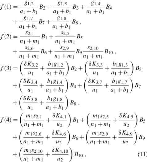
stress as defined by Eq. (6), are given by f (1)= g1,2
a1+b1 B2+
g1,3 a1+b1
B3+ g1,4 a1+b1
B4
+ g1,7
a1+b1 B7+
g1,8 a1+b1
B8,
f (2)= s2,1
n1+m1 B1+
s2,5 n1+m1
B5
+ s2,6
n1+m1 B6+
s2,9 n1+m1
B9 s2,10 n1+m1
B10,
f (3)=
δK3,2
u1
+ b1g1,2
a1+b1
B2+
δK3,3
u1
+ b1g1,3
a1+b1
B3
+
δK
3,4 u1
+ b1g1,4
a1+b1
B4+
δK
3,7 u1
+ b1g1,7
a1+b1
B7
+
δK
3,8 u1
+ b1g1,8
a1+b1
B8,
f (4)=
m
1s2,1 n1+m1
+δK4,1
u2
B1+
m
1s2,5 n1+m1
+δK4,5
u2
B5
+
m
1s2,6 n1+m1
+δK4,6
u2
B6+
m
1s2,9 n1+m1
+δK4,9
u2
B9
+
m
1s2,10 n1+m1
+δK4,10
u2
B10, (11)
whose coefficients are provided in Appendix B, whereBi= ψi3=ψi−θi. Note that the f (i) should not be confused
with the Coriolis parameterf0and the parameterf1of Ap-pendix A.
2.3 Estimation of the main parameters
The estimation of the main physical parameters is made as follows. For the atmosphere, the parameterk is related to the surface drag felt by the lower layer of the two-layer QG model. This is estimated based on the Ekman layer theory (p. 115, Vallis, 2006) as
k= d
2D (12)
after dividing byf0, and where D andd are the thickness of the lower atmospheric layer and the thickness of the Ek-man surface layer, respectively. TypicallyDis of the order of 5000 m andd of the order of 100–1000 m. This implies thatkfalls in a range of[0.01,0.1]. Here the value is fixed tok=0.02 (and the other dissipation parameters are fixed toh00=k0=2k). For parameterδ, one can use the estimate done by Nese and Dutton (1993). The dimensional forcing coefficient is given by
ko=
|V|ρaCD
ρoh
, (13)
whereρa andρoare the densities of the air and of the sea water, respectively. h is the thickness of the ocean layer andCD the surface friction coefficient. With CD≈0.001,
-300000 -250000 -200000 -150000 -100000 -50000 0 50000 100000 150000 200000 250000
200000 201200 202400 203600
Αi
Time (days) n=1.5, Θ*=.14, δ=0.0019305
i=1 i=2 i=3 i=4
Fig. 1.Temporal evolution of the four modesAiforθ∗= 0.14andδ= 0.001938.
figure
31
Fig. 1. Temporal evolution of the four modes ofAi forθ∗=0.14
andδ=0.001938.
h≈20–500 m, |V| ≈5–10 m s−1, ρa≈1 kg m−3 and ρo≈ 1000 kg m−3, one gets values (once normalized byf0) in the range[0.0001,0.01]. Note thatCin Eq. (6) is equivalent to C= |V|ρaCD.
For the thermal forcing, the same approach as in Charney and Straus (1980) and in Reinhold and Pierrehumbert (1982) is adopted, through the use of the thermal wind relation.θ∗ is therefore allowed to vary from[0,0.2].
3 Results of the integration of OA-QG-WS v2
In this section, some statistical and dynamical properties of the model are reported as a benchmark. The numerical scheme used is a second-order temporal scheme known as the Heun scheme (see Kalnay, 2003) with a time step of 0.01 time unit. The parameter values used are listed in Table 1, while the behavior of the system is explored by varyingδ andθ∗. The dimensional time unit is equal to 0.11215 days.
3.1 Model trajectories and mean fields
Figure 1 displays the temporal evolution of theAi variables
of the ocean component for about 10 years starting after 200 000 days of integration. Interestingly a long-range vari-ability emerges as in Vannitsem (2014).
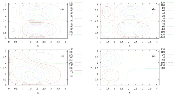
As already alluded in Vannitsem (2014), this new version of the model allows for the development of double gyres. Figure 2 displays the mean streamfunction fields for differ-ent values of the key parametersθ∗=0.077,θ∗=0.10, and θ∗=0.14, after a long integration of about 3.5×10⁸days. Two different initial states in phase space are used forθ∗=
Fig. 2. Average streamfunction field of the ocean forδ=0.001938 andθ∗=0.077 (a), 0.077 (b), 0.10 (c) and 0.14 (d), as obtained from a long integration of about 3.5×10⁸days. Note that (a) and (b) are obtained with the same parameters but different initial states in phase space.
Table 1. Dimensional and nondimensional parameters used in the
coupled ocean–atmosphere model.
Dimensional parameters Nondimensional parameters
L= 5000
π km n=1.5
Lx= 2π Ln α=1
Ly=π L γ= −L2/L2R= −1741
f0=1.032 10−4s−1 h00=k0=2k=0.04
LR= √
g0H
f0 =38 002 m β
0=βL/f
0=0.2498 σ0=0.1
r0=0.0000969 δ= [10−4,10−2]
θ∗= [0.,0.2]
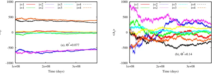
variation of these mean values are illustrated in Fig. 3, for θ∗=0.077 andθ∗=0.14, starting from two different initial conditions. The convergence is very slow due to the natu-ral long-term variability of the ocean embedded in this sys-tem. The presence of different attractors cannot be confirmed or excluded at this stage, due to the blurring of the large natural variability of the system. This analysis would need even longer model integrations, with a higher-order numer-ical scheme in order to better control the numernumer-ical error as suggested by the anonymous referee. Two codes (in For-tran and Lua) used to integrate the model (with the second-order Heun method) and compute these averaged quantities are provided as Supplement and can be used freely, provided proper reference to the source is made.
Figure 4 displays the power spectra of modesψ1andA1, as obtained using a time series of about 73 500 days for θ∗=0.14 (sampled every 0.56075 days, one point every 500
adimensionalized time steps). The atmospheric field displays a flat spectrum for small frequencies and decays at the large ones. The typical timescale of transition between these two regimes is of the order of 30 days for this large-scale atmo-spheric mode. For the oceanic mode, the power spectrum is continuously decaying closely following a power law, indi-cating long-range time dependences (in agreement with the visual inspection of Fig. 1). A change of slope is also visible in this log–log plot, around a timescale of 30 days, reflect-ing the change of statistical properties in the atmosphere. For low frequencies (betweenω=0.0001 andω=0.2, the slope of the decay is close to−2, suggesting a dynamics close to a red noise. For large frequencies, the slope is much sharper with a value close to−4. At low frequencies the ocean acts as an integrator of the “white” noise produced by the atmo-sphere, by analogy with a Brownian motion or an Ornstein– Uhlenbeck process.
3.2 Chaotic dynamics
-1000 -500 0 500 1000
1e+08 2e+08 3e+08
<
Αi
>
Time (days) (a), Θ*=0.077 i=1
i=1 i=2 i=2
i=3 i=3
i=4 i=4
-1000 -500 0 500 1000
1e+08 2e+08 3e+08
<
Αi
>
Time (days) (b), Θ*=0.14 i=1
i=1 i=2 i=2
i=3 i=3
i=4 i=4
Fig. 3.Convergence of the mean values of the oceanic modesAifor(a)θ∗= 0.077,δ= 0.001938and
(b)θ∗= 0.14,δ= 0.001938.
33
Fig. 3. Temporal variation of the mean values of the oceanic modesAi for (a)θ∗=0.077,δ=0.001938 and (b)θ∗=0.14,δ=0.001938.
1e+06 1e+08 1e+10 1e+12 1e+14 1e+16 1e+18 1e+20
1e-05 0.0001 0.001 0.01 0.1 1 10
Power,
ψ1
2 π / Τ
(a)
1e+06 1e+08 1e+10 1e+12 1e+14 1e+16 1e+18 1e+20
1e-05 0.0001 0.001 0.01 0.1 1 10
Power,
Α1
2 π / Τ
(b)
Fig. 4.Power spectra forψ1andA2obtained using a time series of about 73 215 days, forθ∗= 0.14,
δ= 0.001938(= 2×10⁻⁷f
0).
34
Fig. 4. Power spectra forψ1andA2obtained using a time series of about 73 500 days, forθ∗=0.14, andδ=0.001938 (=2×10⁻⁷f0).
be shown that there exists a set of (characteristic) vectors,
ui(t ), i=1, . . . , n, and a corresponding set of
(characteris-tic) numbers,σi, quantifying the degree of amplification of
small perturbations,δxi(t ), along these vectors. These
char-acteristic numbers are known as the Lyapunov exponents and are given by
σi= lim t→∞
1 t ln
|δx i(t )|
|δxi(0)|
. (14)
If one of these exponents is positive, then the system is sensitive to initial conditions and the solution is chaotic. If the largest one is 0 and the others negative, then the solution is periodic. If the two largest exponents are 0 and the others negative, the solution lives on a 2-torus. Practically it is not necessary to know these specific vectors,ui(t ), i=1, . . . , n,
to get the Lyapunov exponents and any basis of indepen-dent vectors can be used, because the amplification of any L-dimensional volume in phase space will amplify on aver-age with a rate equal to the sum of the firstLLyapunov expo-nents (e.g., Legras and Vautard, 1996). Numerically one uses a basis which is regularly orthonormalized in order to avoid the collapse of all the vectors along the dominant instability direction (e.g., Parker and Chua , 1989).
One of the main properties of this new version of the model is the possibility of having a “large” number of positive Lyapunov exponents, and hence a “large” attrac-tor dimension. Figure 5a displays the variations of the first,
second and third Lyapunov exponents as a function of θ∗ forδ=0.001938. For values ofθ∗ smaller than 0.055, sta-ble steady states are found with a set of four negative Lya-punov exponents of very small amplitude (e.g., for θ∗=
-0.1 0 0.1 0.2 0.3 0.4 0.5 0.6
0 0.02 0.04 0.06 0.08 0.1 0.12 0.14 0.16 0.18
σ1, 2, 3
thermal forcing, Θ*
(a) 1st exponent
2nd exponent 3rd exponent
0 0.1 0.2 0.3 0.4 0.5 0.6 0.7 0.8
0 0.02 0.04 0.06 0.08 0.1 0.12 0.14 0.16 0.18
-1 0 1 2 3 4 5
KS entropy
Number of positive exponents
thermal forcing, Θ*
(b) K-S entropy Nbr of positive exponents
Fig. 5.Values of the 3 first Lyapunov exponents,(a), and the Kolmogorov–Sinai entropy and the number of positive Lyapunov exponents,(b), as a function ofθ∗forδ= 0.001938.
35
Fig. 5. Values of the first three Lyapunov exponents, (a), and the Kolmogorov–Sinai entropy and the number of positive Lyapunov exponents, (b), as a function ofθ∗forδ=0.001938.
model has therefore more flexibility since one can easily get different configurations in terms of dynamical instability, by changing the main parameterθ∗. A detailed analysis of the transitions from quasi-periodic motions to chaotic behaviors will be investigated in the future as in recent works (Broer et al., 2011; Sterk et al., 2010, among others).
Figure 6 displays the dependence of the amplitudes of the Lyapunov exponents and the number of positive ex-ponents as a function of the coupling parameter δ, for three different values of θ∗. As in Vannitsem (2014), the trends of the Lyapunov properties as a function of δ can be very different for different values of θ∗. The values of the exponents for θ∗=0.0825 are very sen-sitive to δ, with sharp transition from (quasi-)periodic solutions to chaotic behaviors around δ=0.009. This in-teresting feature suggests thatδ plays a crucial role in set-ting up the transition from nonchaotic to chaotic regimes in the coupled system. A full understanding of this transition should be obtained through a systematic analysis of the bi-furcation diagram of this system (and it will be the subject of a future investigation). Forθ∗=0.10 andθ∗=0.14 an in-crease is found for the first two exponents (but very weak for θ∗=0.14), while a third positive one emerges when δ is increased. Interestingly, these results confirm the tendency already reported in van Veen (2003), indicating that the pres-ence of the ocean has a stronger influpres-ence on the dynamics of the atmosphere close to the periodic windows.
The sensitivity toδis also illustrated in Fig. 6d in which the Kolmogorov–Sinai entropy is shown, displaying a sys-tematic increase for the three values explored. These trends are opposite to those discovered in Nese and Dutton (1993). Their results are most probably associated with the way the heat is transported in the ocean basin and then transferred to-ward the atmosphere in their model, a feature not present in our model. This is worth investigating further in the future by adding thermal exchanges between the atmosphere and the ocean.
For all the cases explored, the number of positive Lya-punov exponents also has a tendency to increase with the am-plitude of the couplingδ. This feature is similar to what was
found in OA-QG-WS v1, further reflecting the importance of the coupling between the ocean and the atmosphere.
To further understand this increase of instability as a func-tion of the coupling parameter, the mean absolute amplitude of the (backward) Lyapunov vectors along the different vari-ables of the coupled system has been computed. Figure 7 displays the results for the first (backward) Lyapunov vector (see Legras and Vautard, 1996) corresponding to the domi-nant Lyapunov exponent for the same parameter as in Fig. 5c and for three different values ofδ. The first 10 points corre-spond to the barotropic variables of the system, the next 10 points to the baroclinic ones, and the last 4 points to the ocean variables. Clearly the projections along the atmospheric vari-ables do not change as a function of the couplingδ, contrary to the projection along the ocean variables. A similar picture is found for the other backward Lyapunov vectors. This sug-gests that the increase of instability is mainly associated with an increase of the projection of the vectors along the ocean variables, and not the baroclinic or barotropic instability within the atmosphere. This conjecture is worth investigating further in the future through a detailed analysis of the bifur-cation diagram and of the characteristic vectors (also called covariant vectors) of the system, which are (nonorthogonal) intrinsic directions of instabilities (see Legras and Vautard, 1996).
4 Conclusions
0 0.02 0.04 0.06 0.08 0.1 0.12
0.002 0.004 0.006 0.008 0.01
σ1,2,3
Coupling parameter
(a) 1st exponent
2nd exponent 3rd exponent
0 0.05 0.1 0.15 0.2 0.25
0.002 0.004 0.006 0.008 0.01
σ1,2,3
Coupling parameter
(b) 1st exponent 2nd exponent 3rd exponent
0 0.05 0.1 0.15 0.2 0.25 0.3 0.35 0.4 0.45
0.002 0.004 0.006 0.008 0.01
σ1,2,3
Coupling parameter
(c) 1st exponent
2nd exponent 3rd exponent
0 0.1 0.2 0.3 0.4 0.5 0.6
0.002 0.004 0.006 0.008 0.01
KS entropy
Coupling parameter
(d) Θ* = 0.0825
Θ* = 0.10 Θ* = 0.14
Fig. 6.
Values of the 3 first Lyapunov exponents as a function of the coupling parameter
δ
for
θ
∗= 0
.
0825
(a),
0
.
10
(b), and
0
.
14
(c).
(d)
Variation of the Kolmogorov–Sinai entropy as a function of
δ
for the same
values of
θ
∗.
36
Fig. 6. Values of the first three Lyapunov exponents as a function of the coupling parameterδforθ∗=0.0825 (a), 0.10 (b), and 0.14 (c).
(d) Variation of the Kolmogorov–Sinai entropy as a function ofδfor the same values ofθ∗.
1e-11 1e-10 1e-09 1e-08 1e-07 1e-06 1e-05 0.0001 0.001 0.01 0.1 1
0 5 10 15 20 25
|LV
1,i
|
ψ1...10, Θ1...10, A1..4
δ = 0.0004826 δ = 0.0019305 δ = 0.009653
Fig. 7.Mean absolute amplitude of the first (backward) Lyapunov vector along the variables of the system, from 1 to 10,ψi, from 11 to 20,θi, and from 21 to 24,Ai, as obtained after an integration of106 days.
37
Fig. 7. Mean absolute amplitude of the first (backward) Lyapunov
vector along the variables of the system, from 1 to 10,ψi, from 11
to 20,θi, and from 21 to 24,Ai, as obtained after an integration of
106days. The other parameters as in Fig. 6c.
attractors (associated with a larger number of positive Lya-punov exponents) can be found, and double gyres can de-velop in the ocean basin in the presence of a chaotic atmo-sphere.
The Lyapunov instability properties of the flow have also been explored. Interestingly, for the set of parameters chosen, a transition from periodic to chaotic regimes occurs at a value
of the bifurcation parameter close toθ∗=0.065. Close to this value, the dynamics is also highly sensitive to the val-ues of the coupling parameterδ, with a possibility of a sharp transition from periodic to chaotic regimes. For large values of θ∗, the dominant exponent is less sensitive toδ, in con-trast to the lowest amplitude positive exponent. In addition, the number of positive Lyapunov exponents has a tendency to increase withδregardless of whatθ∗is, suggesting an in-crease of the dimension of its attractor in phase space. The latter characteristic was also found in the first version (OA-QG-WS v1) of the model.
Appendix A
Coefficients of the ocean component of the model
a1= 3π 8αn(α
2−n2/4−1+γ ), b 1=
8αn 3π u1 c1=
αβ0
u1
−β
0
2α, d1=
−4nβ0
3π u1
−3πβ
0
8n e1= −(r0+δ)
(α2−n2/4−1)3π 8αn+
8αn 3π u1
,
f1= −(r0+δ)
1−(α
2−n2−1) u1
c0= αβ0
u1
, d0=
−4nβ0 3π u1 e0= −(r0+δ)
8αn 3π u1
, v0=(r0+δ)
(α2−n2−1) u1
n1= 3π 8αn(α
2−n2/4−4+γ ), m 1=
8αn 3π u2 o1=
−4nβ0 3π u2
−3πβ
0
8n , p1= αβ0
u2
− β
0
2α q1= −(r0+δ)
(α2−n2/4−4)3π 8αn+
8αn 3π u2
,
r1= −(r0+δ)
1−(α
2−n2−4) u2
o0=
−4nβ0 3π u2
, p0= αβ0
u2
q0= −(r0+δ) 8αn 3π u2
, r0=(r0+δ)
(α2−n2−4) u2
u1=α2−n2−1+γ , u2=α2−n2−4+γ and
L112= 3π
8αn(C112+C121), L114= 3π
8αn(C114+C141) L123=
3π
8αn(C123+C132), L134= 3π
8αn(C134+C143) L312=
1 u1
(C312+C321), L314= 1 u1
(C314+C341)
L323= 1 u1
(C323+C332), L334= 1 u1
(C334+C343)
L211= 3π
8αnC211, L233= 3π 8αnC233 L213=
3π
8αn(C213+C231), L413= 1 u2
(C413+C431)
L411= 1 u2
C411, L433= 1 u2
C433
where
Cij k= n 2π2
π Z
0 dy0
2π/n Z
0
dx0e2αx0φiJ (φj,∇2φk)
giving
C112= 2 π
αn4(4α2−3n2−48) (4α2+9n2)(4α2+n2)(1+e
−α2π/n),
C121= 1 π
αn4(−4α2+15n2+24) (4α2+9n2)(4α2+n2) (1+e
−α2π/n),
C114= 1 π
αn4(α2+n2−12) (α2+4n2)(α2+n2)(1−e
−α2π/n),
C141= − 1 4π
αn4(2α2−19n2−12) (α2+4n2)(α2+n2) (1−e
−α2π/n),
C123= − 1 2π
n4(α4−2α2n2−6α2−3n4−3n2) α(α2+4n2)(α2+n2) (1−e−α2π/n),
C132=
−1
8π
n4(16α2n2−8α4+96α2+3n4+48n2) α(α2+4n2)(α2+n2)
(1−e−α2π/n), C134=
−8
π
αn4(39n4−16n2(−21+α2)−16α2(−12+α2)) (4α2+n2)(4α2+9n2)(4α2+25n2) (1+e−α2π/n),
C143=
4 π
αn4(303n4−16α2(−6+α2)+8n2(21+13α2)) (4α2+n2)(4α2+9n2)(4α2+25n2) (1+e−α2π/n),
C231= 1 8π
n4(−4α4−22α2n2+3n4+12n2) α(α2+4n2)(α2+n2) (1−e−α2π/n),
C213= − 1 2π
n4(α4+4α2n2+3n4+3n2) α(α2+4n2)(α2+n2) (1−e
−α2π/n),
C211= − 1 π
n4α
(4α2+n2)(1+e
−α2π/n),
C233= − 4 π
αn4
(4α2+n2)(1+e
−α2π/n),
C312= 1 8π
n4(8α4−28α2n2−96α2+3n4+48n2) α(α2+4n2)(α2+n2)
(1−e−α2π/n), C321= −
1 8π
n4(4α4−44α2n2−24α2+3n4+12n2) α(α2+4n2)(α2+n2)
(1−e−α2π/n), C323=
−4
π
αn4(16α4−128α2n2−345n4−120n2−96α2) (4α2+n2)(4α2+9n2)(4α2+25n2) (1+e−α2π/n),
C332= 8 π
(1+e−α2π/n), C314=
8 π
αn4(16α4−8α2n2−81n4−144n2−192α2) (4α2+n2)(4α2+9n2)(4α2+25n2) (1+e−α2π/n),
C341= − 4 π
αn4(16α4−248α2n2−63n4−72n2−96α2) (4α2+n2)(4α2+9n2)(4α2+25n2) (1+e−α2π/n),
C334=
−4
π
αn4(−α2+3n2+12) (α2+n2)(α2+9n2) (1−e
−α2π/n),
C343= 1 π
αn4(−2α2+30n2+12) (α2+n2)(α2+9n2) (1−e
−α2π/n),
C433= − 2 π
n4α
(α2+n2)(1−e
−α2π/n),
C411= − 1 2π
n4α
(α2+n2)(1−e
−α2π/n),
C431= − 4 π
αn4(16α4+136α2n2+33n4−48n2) (4α2+n2)(4α2+9n2)(4α2+25n2) (1+e−α2π/n),
C413= − 4 π
αn4(16α4+112α2n2+183n4+48n2) (4α2+n2)(4α2+9n2)(4α2+25n2) (1+e−α2π/n).
Appendix B
Coefficients of the coupling between the ocean and the atmosphere
g1,2=δ
3π
8αnK1,2− K3,2
u1
,
s2,1=δ
3π
8αnK2,1− K4,1
u2
g1,3=δ
3π
8αnK1,3− K3,3
u1
,
s2,5=δ
3 π 8αnK2,5−
K4,5 u2
g1,4=δ
3π
8αnK1,4− K3,4
u1
,
s2,6=δ
3π
8αnK2,6− K4,6
u2
g1,7=δ
3π
8αnK1,7− K3,7
u1
,
s2,9=δ
3π
8αnK2,9− K4,9
u2
g1,8=δ
3π
8αnK1,8− K3,8
u1
,
s2,10=δ
3π
8αnK2,10− K4,10
u2
with
Ki,j= n 2π2
π Z
0 dy0
2π/n Z
0
dx0e2αx0φi∇2Fj
giving
K1,2= − 2 π
(n2+1)n2(4α2−3n2) (4α2+9n2)(4α2+n2)(1+e
α2π/n),
K1,3= 16
π
(n2+1)αn3
(4α2+9n2)(4α2+n2)(1+e
α2π/n),
K1,4= 16
√
2 3π2
n2
(4α2+n2)(1+e
α2π/n),
K2,1= − 8
√
2 3π2
n2
(4α2+n2)(1+e
α2π/n),
K2,5= − 2 π
(n2+4)n2(4α2−3n2) (4α2+9n2)(4α2+n2)(1+e
α2π/n),
K2,6= 16
π
(n2+4)αn3
(4α2+n2)(4α2+9n2)(1+e
α2π/n),
K3,2=
−1
π
n2(n2+1) (α2+4n2)(1−e
α2π/n),
K3,3= 2 π
n3(n2+1) α(α2+4n2)(1−e
α2π/n),
K3,4= 8
√
2 3π2
n2
(α2+n2)(1−e
α2π/n),
K4,1= − 4
√
2 3π2
n2
(α2+n2)(1−e
α2π/n),
K4,5=
−1
π
n2(n2+4) (α2+4n2)(1−e
α2π/n),
K4,6= 2 π
n3(n2+4) α(α2+4n2)(1−e
α2π/n),
K1,7= n2
π
(30n2−8α2)(4n2+1) (4α2+25n2)(4α2+9n2)(1+e
α2π/n),
K1,8= 32αn3
π
(4n2+1)
(4α2+25n2)(4α2+9n2)(1+e
α2π/n),
K2,9= 4n2
π
(30n2−8α2)(n2+1) (4α2+25n2)(4α2+9n2)(1+e
α2π/n),
K2,10= 128αn3
π
(n2+1)
(4α2+25n2)(4α2+9n2)(1+e
α2π/n),
K3,7= − n2
π
(α2−3n2)(4n2+1) (α2+n2)(α2+9n2)(1−e
α2π/n),
K3,8= 4αn3
π
(4n2+1)
(α2+n2)(α2+9n2)(1−e
α2π/n),
K4,9= − 4n2
π
(α2−3n2)(n2+1) (α2+n2)(α2+9n2)(1−e
K4,10= 16αn3
π
(n2+1)
(α2+n2)(α2+9n2)(1−e
α2π/n),
and where theBi =ψi3=ψi−θiare the atmospheric
stream-function variables (mode amplitudes) in the lower layer. The coupling term appearing in the lower layer of the at-mospheric model equations,kd∇29, is expressed in theith atmospheric ordinary differential equation asP
jDijAj
us-ing the inner product of Eq. (4), where D1,2=
−2
√
2 3π2
n2(4α2+n2+16) (4α2+n2) (1+e
−α2π/n),
D1,4=
−4
√
2 3π2
n2(α2+n2+4) (α2+n2) (1−e
−α2π/n),
D2,1= n π
(−8α4n−28α2n3−8α2n+3/2n5+6n3) (4α2+n2)(4α2+9n2)
(1+e−α2π/n), D2,3=
−n2
π
(α2+5n2+1) (α2+4n2) (1−e
−α2π/n),
D3,1=
−16
π
αn3(n2+1)
(4α2+n2)(4α2+9n2)(1+e
−α2π/n),
D3,3=
−2
π
n3(n2+1) α(α2+4n2)(1−e
−α2π/n),
D4,1= 4
√
2 3π2
n2(α2+n2/4+1) (4α2+n2) (1+e
−α2π/n),
D4,3= 2
√
2 3π2
n2(α2+n2+1) (α2+n2) (1−e
−α2π/n),
D5,2= n2 2π
(−16α2(α2+4)+3n4−8n2(7α2−6)) (4α2+n2)(4α2+9n2) (1+e−α2π/n),
D5,4=
−n2
π
(α2+5n2+4) (α2+4n2) (1−e
−α2π/n),
D6,2=
−16
π
αn3(n2+4)
(4α2+n2)(4α2+9n2)(1+e
−α2π/n),
D6,4=
−2
π
n3(n2+4) α(α2+4n2)(1−e
−α2π/n),
D7,1= n π
(−8α4n−100α2n3−8α2n+15/2n5+30n3) (4α2+25n2)(4α2+9n2)
(1+e−α2π/n), D7,3=
n2 π
(−α4−14α2n2−α2+3n4+3n2) (α2+n2)(α2+9n2) (1−e
−α2π/n),
D8,1= − 32n3α
π
(4n2+1)
(4α2+25n2)(4α2+9n2)(1+e
−α2π/n),
D8,3= − 4αn3
π
(4n2+1)
(α2+n2)(α2+9n2)(1−e
−α2π/n),
D9,2= n2 2π
(−16α2(α2+4)+15n4−40(5α2−6)n2) (4α2+25n2)(4α2+9n2)
(1+e−α2π/n), D9,4=
n π
(−14α2n3−nα4−4nα2+3n5+12n3) (α2+n2)(α2+9n2)
(1−e−α2π/n), D10,2= −
128n3α π
(n2+1)
(4α2+25n2)(4α2+9n2)(1+e
−α2π/n),
D10,4= − 16n3α
π
(n2+1)
(α2+n2)(α2+9n2)(1−e
Supplementary material related to this article is available online at http://www.geosci-model-dev.net/7/ 649/2014/gmd-7-649-2014-supplement.zip.
Acknowledgements. This work is partially supported by the Belgian Federal Science Policy Office under contracts SD/CA/04A and BR/121/A2/STOCHCLIM.
Edited by: J. Annan
References
Arnold, L., Imkeller, P., and Wu, Y.: Reduction of deterministic cou-pled atmosphere-ocean models to stochastic ocean models: a nu-merical case study of the Lorenz–Maas system, Dynam. Syst., 18, 295–350, 2003.
Birchfield, G. E.: A coupled ocean–atmosphere climate model: tem-perature versus salinity effects on the thermohaline circulation, Clim. Dynam., 4, 57–71, 1989.
Broer, H. W., Dijkstra, H. A., Simó, C., Sterk, A. E., and Vitolo, R.: The dynamics of a low-order model for the Atlantic Multidecadal Oscillation, DCDS-B, 16, 73–102, 2011.
Charney, J. G. and DeVore, J. G.: Multiple flow equilibria in the atmosphere and blocking, J. Atmos. Sci., 36, 1205–1216, 1979. Charney, J. G. and Straus, D. M.: Form-drag instability, multiple
equilibria and propagating planetary waves in baroclinic, oro-graphically forced, planetary wave systems, J. Atmos. Sci., 37, 1157–1176, 1980.
Carrassi, A. and Vannitsem, S.: Accounting for model error in variational data assimilation: A deterministic formulation, Mon. Weather Rev., 138, 3369–3386, 2010.
Carrassi, A. and Vannitsem, S.: Treatment of the model error due to unresolved scales in sequential data assimilation, Int. J. Bif. Chaos, 21, 3619–3626, 2011.
Crucifix, M.: Oscillators and relaxation phenomena in Pleistocene climate theory, Philos. T. Roy. Soc. A, 370, 1140–1165, 2012. Deremble, B., Simonnet, E., and Ghil, M.: Multiple equilibria and
oscillatory modes in a mid-latitude ocean-forced atmospheric model, Nonlinear Proc. Geoph., 19, 479–499, 2012.
Dijkstra, H. A. and Ghil, M.: Low-frequency variability of the large-scale ocean circulation: a dynamical system approach, Rev. Geo-phys., 43, RG3002, doi:10.1029/2002RG000122, 2005. Goswami, B. N., Selvarajan, S., and Krishnamurty, V.: Mechanisms
of variability and predictability of the tropical coupled ocean– atmosphere system, Proc. Indian Acad. Sci., 102, 49–72, 1993. Imkeller, P. and Monahan, A. H.: Conceptual stochastic climate
models, Stoch. Dynam., 2, 311–326, 2002.
Jiang, S., Jin, F.-F., and Ghil, M.: Multiple equilibria, periodic, and aperiodic solutions in a wind-driven, double-gyre, shallow-water model, J. Phys. Oceanogr., 25, 764–786, 1995.
Kalnay, E.: Atmospheric Modeling, Data Assimilation and Pre-dictability, Cambridge University Press, Cambridge, 2003. Legras, B. and Vautard, R.: A guide to Lyapunov vectors, in:
Predictability, Vol. 1, edited by: Palmer, T., ECMWF Seminar, ECMWF, Reading, UK, 135–146, 1996.
Lorenz, E. N.: Deterministic nonperiodic flow, J. Atmos. Sci., 20, 130–141, 1963.
Lorenz, E. N.: Irregularity: a fundamental property of the atmo-sphere, Tellus A, 36, 98–110, 1984a.
Lorenz, E. N.: Formulation of a low-order model of a moist general circulation, J. Atmos. Sci., 41, 1933–1945, 1984b.
Lucarini, V., Faranda, D., Turchetti, G., and Vaienti, S.: Ex-treme value theory for singular measures, Chaos, 22, 023135, doi:10.1063/1.4718935, 2012.
Maas, L.: A simple model for the three-dimensional, thermally and wind-driven ocean circulation, Tellus A, 46, 671–680, 1994. Nese, J. M. and Dutton, J. A.: Quantifying predictability variations
in a low-order ocean–atmosphere model: a dynamical system ap-proach, J. Climate, 6, 185–203, 1993.
Nicolis, C.: Probabilistic aspects of error growth in atmospheric dy-namics, Q. J. Roy. Meteorol. Soc., 118, 553–568, 1992. Nicolis, C. and Nicolis, G.: Environmental fluctuation effects on the
global energy balance, Nature, 281, 132–134, 1979.
Nicolis, G. and Nicolis, C.: Foundations of complex systems: emer-gence, information and prediction, World Scientific, Singapore, 367 pp., 2012.
Paillard, D.: The timing of Pleistocene glaciations from a simple multiple-state climate model, Nature, 391, 378–381, 1998. Parker, T. S. and Chua, L. O.: Practical Numerical Algorithm for
Chaotic Systems, Springer-Verlag, New York, 348 pp., 1989. Palmer, T. N.: Extended range atmospheric prediction and the
Lorenz model, B. Am. Meteorol. Soc., 74, 49–65, 1993. Pena, M. and Kalnay, E.: Separating fast and slow modes in coupled
chaotic systems, Nonlinear Proc. Geoph., 11, 319–327, 2004. Pierini, S.: Low-frequency variability, coherence resonance, and
phase selection in a low-order model of the wind-driven ocean circulation, J. Phys. Oceanogr., 41, 1585–1604, 2011.
Pires, C., Vautard, R., and Talagrand, O.: On extending the limits of variational assimilation in nonlinear chaotic systems, Tellus A, 48, 96–121, 1996.
Reinhold, B. B. and Pierrehumbert, R. T.: Dynamics of weather regimes: quasi-stationary waves and blocking, Mon. Weather Rev., 110, 1105–1145, 1982.
Reinhold, B. B. and Pierrehumbert, R. T.: Corrections to “Dynamics of weather regimes: quasi-stationary waves and blocking”, Mon. Weather Rev., 113, 2055–2056, 1985.
Roebber, P. J.: Climate variability in a low-order coupled atmosphere-ocean model, Tellus A, 47, 473–494, 1995. Saltzman, B.: Finite amplitude free convection as an initial value
problem – I, J. Atmos. Sci., 19, 329–341, 1962.
Simonnet, E. and Dijkstra, H. A.: Spontaneous generation of low-frequency modes of variability in the wind-driven ocean circula-tion, J. Phys. Oceanogr., 32, 1747–1762, 2002.
Simonnet, E., Ghil, M., and Dijkstra, H. A.: Homoclinic bifurca-tions in the quasi-geostrophic double-gyre circulation, J. Mar. Res., 63, 931–956, 2005.
Snyder, C. and Hamill, T.: Leading Lyapunov vectors of a turbu-lent jet in a quasigeostrophic model, J. Atmos. Sci., 60, 683–688, 2003.
Sprott, J. C.: Elegant Chaos, World Scientific, Singapore, 285 pp., 2010.
Stommel, H.: Thermohaline convection with two stable regimes of flow, Tellus, 13, 224–230, 1961.
Trevisan, A.: Statistical properties of predictability from atmo-spheric analogs and the existence of multiple flow regimes, J. Atmos. Sci., 52, 3577–3592, 1995.
Trevisan, A., Pancotti, F., and Molteni, F.: Ensemble prediction in a model with flow regimes, Q. J. Roy. Meteorol. Soc., 127, 343– 358, 2001.
Vallis, G.: Conceptual models of El Nino and the Southern Oscilla-tion, J. Geophys. Res., 93, 13979–13991, 1988.
Vallis, G.: Amospheric and Oceanic Fluid Dynamics, Cambridge University Press, UK, 745 pp., 2006.
Van Schaeybroeck, B. and Vannitsem, S.: Post-processing through linear regression, Nonlinear Proc. Geoph., 18, 147–160, 2011. Vannitsem, S.: A unified linear model output statistics scheme for
both deterministic and ensemble forecasts, Q. J. Roy. Meteorol. Soc., 135, 1801–1815, 2009.
Vannitsem, S.: Dynamics and predictability of a low-order wind-driven ocean–atmosphere coupled model, Clim. Dynam., 42, 1981–1998, doi:10.1007/s00382-013-1815-8, 2014.
Vannitsem, S. and Nicolis, C.: Lyapunov vectors and error growth patterns in a T21L3 quasigeostrophic model, J. Atmos. Sci. 54, 347–361, 1997.
van Veen, L.: Overturning and wind driven circulation in a low-order ocean–atmosphere model, Dynam. Atmos. Oceans, 37, 197–221, 2003.
Veronis, G.: An analysis of wind-driven ocean circulation with a limited number of Fourier components, J. Atmos. Sci., 20, 577– 593, 1963.
Wittenberg, A. T. and Anderson, J. L.: Dynamical implications of prescribing part of a coupled system: Results from a low–order model, Nonlinear Proc. Geoph., 5, 167–179, doi:10.5194/npg-5-167-1998, 1998.