www.geosci-model-dev.net/8/261/2015/ doi:10.5194/gmd-8-261-2015
© Author(s) 2015. CC Attribution 3.0 License.
The Global Gridded Crop Model Intercomparison: data and
modeling protocols for Phase 1 (v1.0)
J. Elliott1, C. Müller2, D. Deryng3, J. Chryssanthacopoulos4, K. J. Boote5, M. Büchner2, I. Foster1, M. Glotter6, J. Heinke7,2,14, T. Iizumi8, R. C. Izaurralde9, N. D. Mueller10, D. K. Ray11, C. Rosenzweig12, A. C. Ruane12, and J. Sheffield13
1University of Chicago & Argonne Natl. Lab Computation Institute, Chicago, Illinois, USA 2Potsdam Institute for Climate Impact Research, Potsdam, Germany
3Tyndall Centre, University of East Anglia, Norwich, UK
4Columbia University Center for Climate Systems Research, New York, New York, USA 5University of Florida Department of Agronomy, Gainesville, Florida, USA
6University of Chicago Department of Geophysical Science, Chicago, Illinois, USA 7International Livestock Research Institute, Nairobi, Kenya
8National Institute for Agro-Environmental Sciences, Tsukuba, Ibaraki, Japan
9University of Maryland Dept. of Geographical Sciences, College Park, Maryland, USA 10Harvard University Center for the Environment, Cambridge, Massachusetts, USA 11University of Minnesota Institute for the Environment, Saint Paul, Minnesota, USA 12NASA Goddard Institute for Space Studies, New York, New York, USA
13Princeton University Dept. Civil & Environ. Engineering, Princeton, New Jersey, USA
14CSIRO (Commonwealth Scientific and Industrial Research Organization), St Lucia QLD 4067, Australia Correspondence to: J. Elliott ([email protected]) and C. Müller ([email protected])
Received: 3 June 2014 – Published in Geosci. Model Dev. Discuss.: 15 July 2014
Revised: 19 November 2014 – Accepted: 23 December 2014 – Published: 11 February 2015
Abstract. We present protocols and input data for Phase 1 of the Global Gridded Crop Model Intercomparison, a project of the Agricultural Model Intercomparison and Improvement Project (AgMIP). The project includes global simulations of yields, phenologies, and many land-surface fluxes using 12– 15 modeling groups for many crops, climate forcing data sets, and scenarios over the historical period from 1948 to 2012. The primary outcomes of the project include (1) a de-tailed comparison of the major differences and similarities among global models commonly used for large-scale climate impact assessment, (2) an evaluation of model and ensemble hindcasting skill, (3) quantification of key uncertainties from climate input data, model choice, and other sources, and (4) a multi-model analysis of the agricultural impacts of large-scale climate extremes from the historical record.
1 Introduction
Climate change presents a significant risk for agricultural productivity in many key regions, even under relatively op-timistic scenarios for near-term mitigation efforts (Rosen-zweig et al., 2014). Consistent global-scale evaluation of crop productivity is essential for assessing the likely impacts of climate change and identifying system vulnerabilities and potential adaptations. Over the last several years, many re-search groups around the world have developed global grid-ded crop models (GGCMs) to simulate crop productivity and climate impacts at relatively high spatial resolution over con-tinental and global extents, with a huge diversity of method-ologies and assumptions leading to a wide range of results.
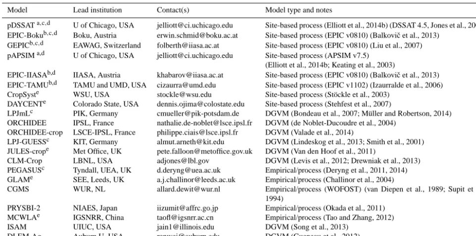
Intercompari-Table 1. Models and groups engaged thus far for GGCMI.
Model Lead institution Contact(s) Model type and notes
pDSSATa,c,d U of Chicago, USA [email protected] Site-based process (Elliott et al., 2014b) (DSSAT 4.5, Jones et al., 2003) EPIC-Bokub,c,d Boku, Austria [email protected] Site-based process (EPIC v0810) (Balkoviˇc et al., 2013)
GEPICb,c,d EAWAG, Switzerland [email protected] Site-based process (EPIC v0810) (Liu et al., 2007)
pAPSIMa,d U of Chicago, USA [email protected] Site-based process (APSIM v7.5) (Elliott et al., 2014b; Keating et al., 2003)
EPIC-IIASAb,d IIASA, Austria [email protected] Site-based process (EPIC v0810) (Balkoviˇc et al., 2013) EPIC-TAMUb,d TAMU and UMD, USA [email protected] Site-based process (EPIC v1102) (Izaurralde et al., 2006) CropSyste WSU, USA [email protected] Site-based process (Stöckle et al., 2003)
DAYCENTe Colorado State, USA [email protected] Site-based process (Stehfest et al., 2007)
LPJmLc PIK, Germany [email protected] DGVM (Bondeau et al., 2007; Müller and Robertson, 2014) ORCHIDEE IPSL, France [email protected] DGVM (de Noblet-Ducoudre et al., 2004)
ORCHIDEE-crop LSCE-IPSL, France [email protected] DGVM (Valade et al., 2014)
LPJ-GUESSc KIT, Germany [email protected] DGVM (Lindeskog et al., 2013; Smith et al., 2001) JULES-crope Met Office, UK [email protected] DGVM (Van den Hoof et al., 2011)
CLM-Crop LBNL, USA [email protected] DGVM (Levis et al., 2012; Drewniak et al., 2013) PEGASUSc Tyndall, UEA, UK [email protected] Empirical/process (Deryng et al., 2011, 2014) GLAMe SEE, Leeds, UK [email protected] Empirical/process (Challinor et al., 2004)
CGMS WUR, NL [email protected] Empirical/process (WOFOST) (van Diepen et al., 1989; Supit et al., 1994)
PRYSBI-2 NIAES, Japan [email protected] Empirical/process (Okada et al., 2011) MCWLAe IGSNRR, China [email protected] Empirical/process (Tao and Zhang, 2012)
ISAM UIUC, USA [email protected] DGVM (Song et al., 2013)
DLEM-Ag Auburn U, USA [email protected] DGVM (Gueneau et al., 2012)
apDSSAT and pAPSIM are both part of the parallel System for Integrating Impact Models and Sectors (pSIMS) framework, using inputs and assumptions harmonized as closely as is possible, allowing
for a more direct comparison of inter-model differences.bFour contributing GGCMs are built from the field-scale EPIC model and will be used for detailed explorations of the effects of different assumptions and configurations within the same model.cModel participating in the 2012/2013 AgMIP/ISI-MIP Fast Track.dEPIC-, DSSAT-, and APSIM-based models will perform additional scenarios using alternative methods to model evapotranspiration in order to better understand the effect this important model choice has on assessmentseModels expected to participate starting in Phase 2.
son Project (ISI-MIP) (Warszawski et al., 2014) that brought together a group of GGCMs to simulate future crop produc-tivity under various climate change and farm management scenarios (Elliott et al., 2014a; Rosenzweig et al., 2014; Pi-ontek et al., 2014; Nelson et al., 2014). Increased applica-tion of crop growth models for global-scale analyses and the wide variation in model assumptions and projected outputs found in the Fast-Track assessment inspired the launch of the AgMIP GRIDded crop modeling initiative (Ag-GRID) and the Global Gridded Crop Model Intercomparison (GGCMI). We define here the simulation protocol for the first phase of the GGCMI, which is designed to, among other things, en-able comprehensive evaluation of model and ensemble skill – with respect to yield levels, variability, and large-scale ex-treme events – based on comparisons of simulations and ob-servations over the last several decades.
The GGCMI Phase 1 simulation protocol includes partic-ipants that run a number of gridded crop models (listed with contacts and short descriptions in Table 1), driven with con-sistent inputs based on multiple weather data products (to evaluate uncertainties from weather data) and harmonized management practice data (planting date, growing season length, and fertilizer inputs). The results of these different simulation runs will then be compared to three distinct refer-ence data sets derived from census and remote sensing data sources (Ray et al., 2013; Iizumi et al., 2013; FAOSTAT data, 2013). GGCMI is a protocol-based simulation experiment for gridded crop models and is open to the participation of any
model group that simulates crop productivity at the global scale, including models developed for field-scale application, biogeochemical dynamic global vegetation and land-surface scheme models, empirical-process-based hybrid models, and statistical models.
In the modeling protocol presented here, we describe the simulation experiments and priorities, central inputs pro-vided to modelers, required outputs to be propro-vided by mod-eling groups, and data format conventions. GGCMI proto-cols are designed to overlap as much as possible with and contribute to the refinement of the modeling protocols of the next phase of ISI-MIP (ISI-MIP2). Modelers participating in GGCMI can directly participate in ISI-MIP2 if they so de-sire.
2 Simulation experiments, models, and objectives
The primary goals of Phase 1 of the GGCMI are
1. intercomparison of models with and without harmo-nized inputs and assumptions, and with and without ex-plicit nitrogen stress;
2. evaluation of model and ensemble skill over the histori-cal period;
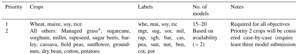
Table 2. Priority 1 and 2 crops in Phase 1, along with the number of models expected to contribute results for each crop.
Priority Crops Labels No. of
models
Notes
1 Wheat, maize, soy, rice whe, mai, soy, ric 15–20 Required for all objectives
2 All others: Managed grass∗, sugarcane, sorghum, millet, rapeseed, sugar beets, bar-ley, cassava, field peas, sunflower, ground-nuts, dry bean, cotton, potatoes
mgr, sug, sor, mil, rap, sgb, bar, cas, pea, sun, nut, ben, cot, pot
Based on availability (>2)
Priority 2 crops will be consid-ered case-by-case (require at least three model submissions)
∗We consider only managed grassland productivity, not unmanaged pasture.
methods, and output processing techniques) in histori-cal crop yield analysis and the implication of these for future climate impact assessment; and
4. multi-model, multi-forcing analysis of the agricultural impacts of large-scale extremes (primarily drought and heat events) in the historical record.
Groups are asked to simulate agricultural productivity for various crops under purely rain-fed as well as fully irrigated conditions for different driving input data sets on weather and management. To avoid overtaxing of modeling groups, we define simulation priorities to facilitate central analyses with an as broad as possible group of GGCMs as well as ad-ditional analyses of more specific questions (the performance of crop models for crops beyond wheat, maize, rice, soy; the influence of weather data uncertainty on model performance; and the impact of different evapotranspiration methodologies on model response and model skill in different regions and agro-climatic zones).
2.1 Crops and management systems to simulate
We define a two-tiered priority structure that takes into ac-count both the crops that are most important for questions of (primarily global) food security and economics, and the crops that are most commonly simulated in available mod-els. The three main cereal crops (maize, wheat, and rice) alone account for about 43 % of total food energy intake (FAOSTAT data, 2013). Along with soybeans, which are the largest single source of oilseeds globally and an essential source of protein and animal feed, these crops have been the focus of most crop yield and climate impact modeling work, and are generally simulated by all the models participating in GGCMI. Thus, we define them as our Priority 1 crops, rep-resenting the minimum set for our analyses (Table 2). Many other crops are important staple food, feed, or energy crops in economically or climate-sensitive regions, and most con-tributing models within GGCMI do simulate one or more of these secondary (or Priority 2) crops. In order to consider as many crops as possible, we ask modelers to supply data on all crops that they can simulate, and consider any crop sim-ulated by at least three models as valid for a multi-model
intercomparison analysis. The participating models cover a broad range of annual crops as well as managed grassland, but provide no modeling capacities for perennial crops (Ta-ble 2).
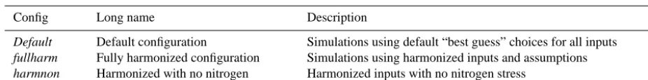
We define three distinct types of model configurations (Ta-ble 3) for the simulations in Phase 1. First, each group is to develop their own “default” configuration based on the management and technology assumptions and inputs they typically use for simulations in the historical period. Each group must also prepare a “harmonized” configuration us-ing input data, parameters, and definitions provided by the GGCMI coordinators. Finally, each model that considers ni-trogen (whether with explicit fertilizers or an empirical cali-bration) is also to be run in a configuration without nitrogen stress, “harmnon”, to allow for direct comparison with mod-els that do not explicitly consider the nitrogen cycle. We de-fine the “hamrnon_firr”, which has zero (or near-zero) stress from both nitrogen and water, as “potential yield” for the pur-pose of defining yield gaps and related analyses.
All modelers are asked to simulate all crops across the globe, irrespective of current cropping areas for purely rain-fed as well as irrigated conditions. This approach allows for addressing uncertainties in assumed distributions of cropland in post-processing analysis. The minimum spatial extent of historical simulations is current agricultural land, and we re-quire that all crops be simulated on all agricultural lands, rather than just on the land where they are currently grown.
We assume that irrigated systems are not limited by fresh-water availability and have no fresh-water losses during con-veyance and application. While the latter assumption has no implications for crop growth, it helps to make reported irri-gation water quantities comparable across models.
above-Table 3. General simulation configurations for Phase 1.
Config Long name Description
Default Default configuration Simulations using default “best guess” choices for all inputs
fullharm Fully harmonized configuration Simulations using harmonized inputs and assumptions
harmnon Harmonized with no nitrogen Harmonized inputs with no nitrogen stress
Table 4. Output variables to be collected during GGCMI Phase 1. The first two variables are to be provided by every model; other variables are to be provided as possible by each model
Variable Variable name∗ Units (and notes)
Mandatory variables to be provided for all simulations
Crop yields yield_<crop> t ha−1yr−1(dry matter)
Applied irrigation water pirrww_<crop> mm yr−1(firr only, assume loss-free con-veyance/application)
Additional variables below are to be provided as possible by each model Total above-ground biomass yield biom_<crop> t ha−1yr−1
Actual growing season evapotranspiration aet_<crop> mm yr−1(season only)
Actual planting date plant-day_<crop> day of year
Days from planting to anthesis anth-day_<crop> days from planting Days from planting to maturity maty-day_<crop> days from planting
Nitrogen application rate initr_<crop> kg ha−1yr−1
Nitrogen leached leach_<crop> kg ha−1yr−1
Nitrous oxide emissions sn2o_<crop> kg N2O-N ha−1
Accumulated precipitation, plant to harvest gsprcp_<crop> mm ha−1yr−1(season only) Growing season incoming solar gsrsds_<crop> W m−2yr−1(season only) Sum of daily mean temperature, planting to harvest sumt_<crop> ◦C days yr−1(season only)
∗<crop>refers to the three-letter variable codes (whe, mai, ric, etc.) from Table 2.
ground biomass, accumulated water applied and transpired, accumulated nitrogen applied and lost through leaching, key phenological dates, and growing season climate characteris-tics. This approach will facilitate better analyses and inter-pretation of results and will allow GGCMI participants to further leverage the archives for scientific deliverables and overall project impacts.
We ask that modelers archive model versions used for the simulations and all primary outputs generated, in order to al-low for reproducibility and facilitate extraction of additional or more detailed (e.g., higher temporal resolution) data that may be found to be necessary for analyses not yet planned.
As far as possible for the models, all modelers should sup-ply yield and irrigation water amounts for at least the four main crops: wheat, maize, rice and soy (Table 2). Simula-tions should be conducted for default and harmonized man-agement assumptions as well as for different weather data sets. If modeling capacities are constrained, modelers should supply at least the four Priority 1 crops (Table 2) and selected weather-management combinations to allow for a compre-hensive model intercomparison across a limited set of sce-narios and for analyses of input and assumption uncertainties
with those models that contributed (Table 5). Priority 1 de-notes the minimum simulations required for participation un-less model capacities do not allow for covering the full spec-trum of Priority 1 simulations (e.g., because not all crops are implemented, or because a model requires special weather data inputs).
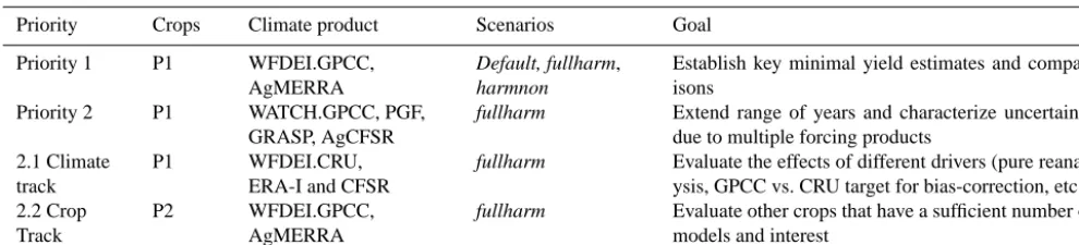
Table 5. Simulation priorities for Phase 1. For climate product descriptions see Table 9.
Priority Crops Climate product Scenarios Goal
Priority 1 P1 WFDEI.GPCC,
AgMERRA
Default, fullharm, harmnon
Establish key minimal yield estimates and compar-isons
Priority 2 P1 WATCH.GPCC, PGF,
GRASP, AgCFSR
fullharm Extend range of years and characterize uncertainty due to multiple forcing products
2.1 Climate track
P1 WFDEI.CRU,
ERA-I and CFSR
fullharm Evaluate the effects of different drivers (pure reanal-ysis, GPCC vs. CRU target for bias-correction, etc.) 2.2 Crop
Track
P2 WFDEI.GPCC,
AgMERRA
fullharm Evaluate other crops that have a sufficient number of models and interest
2.2 Conventions for simulation outputs
In order to facilitate analysis, portability, and processing of outputs, results will be collected in compressed, self-describing NetCDF v4 files with consistent and relatively simple data, metadata, and file-naming conventions de-scribed below.
2.2.1 File names
Each file must contain a single output variable and be named according to the following convention (see definitions in Ta-ble 6):
[model]_[climate]_[clim.scenario]_[sim.scenario]_ [variable]_[crop]_[timestep]_[start-year]_[end-year].nc4
For example,
pdssat_watch_hist_default_noirr_yield_mai_ annual_1958_2001.nc4
2.2.2 Geographical extent
Data must be submitted for the ranges 89.75 to−89.75◦ lati-tude, and−179.75 to 179.75◦longitude. Thus, each file will contain 360 rows and 720 columns for a total of 259 200 grid cells. All ocean grid cells must be filled with the fill value (Table 7). Modelers need not simulate Greenland, the Arctic, or Antarctica but must submit output completely filled for the entire range from latitude 89.75 to−89.75. Output data must be reported row-wise starting at 89.75 and −179.75, and ending at−89.75 and 179.75. As is standard in NetCDF files, latitude, longitude, and time must be included as vari-ables in each file explicitly defining their extent.
2.2.3 Date reporting convention
The analysis of inter-seasonal variability of crop yields is complicated by reporting conventions involving the assign-ment of reported production to calendar years. This issue is especially problematic in the Southern Hemisphere, where harvest sometimes occurs in a window around 31 Decem-ber so that assignment to calendar years based on the harvest date gives double harvests (e.g., one in early January and the next in late December of the same calendar year) in some
years and no harvest in others. The data reporting conven-tion for GGCMI thus is not calendar year but growing sea-son based. That is, results are to be reported as a sequence of growing seasons, irrespective of whether that growing sea-son actually spans 2 calendar years or if harvests occur just before or just after 31 December. Cumulative growing sea-son variables as, e.g., actual evapotranspiration or precipita-tion are to be accumulated over the growing season, again irrespective of any calendar year definitions, and are to be reported in the same sequence as the harvest events (yield, above-ground biomass). The unit of the time dimension of the NetCDF v4 output file is thus “growing seasons since YYYY-01-01 00:00:00” (Table 7). The first season in the file (with value time=1) is then the first complete growing sea-son of the time period provided by the input data without any assumed spin-up data, which equates to the growing season with the first planting after this date. This convention roughly corresponds to an annual reporting scheme but allows for a better separation and analysis of outputs. The artificial sepa-ration of harvest seasons into 2 different calendar years may, however, also be present in observational data and may com-plicate evaluation of model skills in these regions anyway.
3 Central input data
In order to ensure comparability of simulation results across models and to investigate the importance of uncertainties with respect to weather and management data, we sup-ply central input data to all participating modelers. The GGCMI Phase 1 protocols include a set of assumptions, def-initions, and input data products that will be used to harmo-nize participating models as closely as possible in the
full-harm and full-harmnon configurations (Table 8). During project
pre-planning we established data sharing arrangements with leading agricultural data groups that will contribute global high-resolution crop-specific data on key management inputs covering sowing dates, growing season length, fertilizer ap-plication rates (including nitrogen, phosphorus, and potas-sium), manure use, and historical atmospheric CO2
Table 6. Filename conventions for standardized model outputs.
Filename tag [] Values
[model] pdssat, epic-iiasa, lpjml, etc. (see Table 1)
[climate] watch, wfdei.gpcc, wfdei.cru, grasp, agmerra, agcfsr, Princeton (see Table 9)
[clim.scenario] Hist
[sim.scenario] default_firr, fullharm_noirr, etc. (simulation configuration, see Table 3 and irriga-tion setting (firr or noirr))
[variable] yield, pirrww, plant-day, anth-day, etc. (see Table 4)
[crop] mai, soy, whe, ric, mil, sor, etc. (see Table 2)
[timestep] annual
[start-year]_[end-year] 1958_2001, 1980_2009, 1980_2010, etc. (see Table 9)
Table 7. NetCDF file dimension, variable, and attribute info.
Dimension/variable Fill value No. type Units Range
Longitude NA double degrees east −179.75. . . 179.75
Latitude NA double degrees north 89.75. . .−89.75
Time NA double “growing seasons since YYYY-01-01
00:00:00”
(YYYY varies, see Table 9)
1. . .T (T varies, see Table 9).
[variable]_[crop] 1.e+20f float varies (see Tables 2 and 4). varies
are directly comparable to the greatest extent possible. All GGCMI input data described here can be accessed at https: //rdcep.org/ggcmi/data.
3.1 Weather data inputs
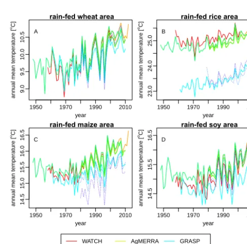
In total we will use six historical retrospective-analysis-based forcing data sets (bias-corrected at monthly timescales against observational products such as CRU and GPCC) and two raw (non-bias-corrected) reanalysis products (Table 9). Within the cropping areas of the major crops, these weather products display some uncertainty with respect to mean and variability of weather variables such as temperature (Fig. 1) and precipitation (Fig. 2). We do not strictly harmonize spin-up procedures for those models that require it; however, we provide the Princeton global forcing data set for years af-ter 1948, and a decade of generic pre-industrial weather that can be used for all preceding years. We also consider two versions of WFDEI, with biases corrected separately using either the GPCC or CRU data as targets, for a total of nine distinct data products and about 350 years of daily data. In total, this collection provides one or more weather data in-puts for every year from 1948 to 2012. All products cover the 30-year period from 1980 to 2009 (which will serve as our primary analysis period) except WATCH (1958–2001) and Princeton (1948–2008). Each data set is provided at daily resolution and one product (WFDEI) is additionally provided at 3-hourly resolution for those models that require sub-daily data.
1950 1970 1990 2010
9.0
9.5
10.0
10.5
rain-fed wheat area
year
ann
ual mean temper
ature [
oC] A
1950 1970 1990 2010
23.0
24.0
25.0
rain-fed rice area
year
ann
ual mean temper
ature [
oC] B
1950 1970 1990 2010
14.5
15.0
15.5
16.0
16.5
rain-fed maize area
year
ann
ual mean temper
ature [
oC] C
1950 1970 1990 2010
14.5
15.5
16.5
rain-fed soy area
year
ann
ual mean temper
ature [
oC] D
WATCH WFDEI
AgMERRA AgCFSR Princeton
GRASP ERAI CFSR
Figure 1. Area-weighted mean of annual temperatures [◦C] for cropping areas for rain-fed wheat (a), rice (b), maize (c), and soy (d).
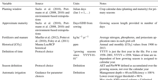
Table 8. Harmonized input variable sources for fullharm and harmnon configurations in Phase 1.
Variable Source Units Notes
Planting window Sacks et al. (2010), Port-mann et al. (2008, 2010) and environment-based extrapola-tions
Julian days (Jan 1=1,. . . )
Crop calendar data (planting and maturity) for pri-mary seasons
Approximate maturity Sacks et al. (2010), Port-mann et al. (2008, 2010) and environment-based extrapola-tions
Days/GDD from sowing
Growing season length provided in number of days
Fertilizers and manure Mueller et al. (2012), Potter et al. (2010), Foley et al. (2011)
kg ha−1yr−1 Average nitrogen, phosphorus, and potassium ap-plication rates in each grid cell
Historical [CO2] Mauna Loa/RCP historical
ppm Annual and monthly [CO2] values from 1900 to 2013.
Definition of time Protocol choice “growing seasons
since YYYY-01-01”
YYYY is just the first year in the file. For a run 1958–2001, YYYY=1958. Values of time are in-dependent of how growing season is assigned to calendar year.
Season definition Protocol choice Definition AET and PirrWW defined as accumulated over the growing season, not over the calendar year Automatic irrigation Guidance for parameter
choices
Definition Management depth=40 cm/Efficiency=100 % Lower event trigger threshold=90 %
Max single AND annual volume=Unlimited
should use the equivalent variable from another data set. As weather variables are bias-corrected individually and there is consequently no consistency between the individual vari-ables within one data set, and as all data refer to the historic period, we assume that the errors introduced by this approach are small.
3.2 Harmonized growing season definitions
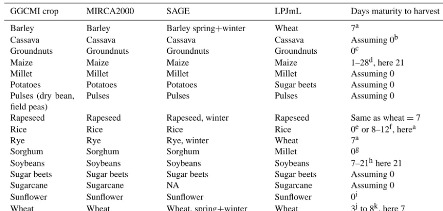
We supply harmonized growing season data (planting and maturity dates) for all Priority 1 crops (wheat, maize, rice, soybeans, see Table 2) plus data for the Priority 2 crops bar-ley, cassava, groundnuts, millet, potatoes, pulses (dry bean, field peas), rapeseed, rye, sorghum, sugar beets, sugarcane, and sunflower. Of the Priority 2 crops, we lack information for cotton, while managed grassland is assumed to grow all year round. We compile growing season data from two ex-isting global crop calendars, MIRCA20001(Portmann et al., 2010) and SAGE2(Sacks et al., 2010), supplementing those data with a rule-based approach as implemented in LPJmL3 (Waha et al., 2012) to provide as much coverage of the global land surface as possible.
1Available for download at ftp://ftp.rz.uni-frankfurt.de/ pub/uni-frankfurt/physische_geographie/hydrologie/public/ data/MIRCA2000/growing_periods_listed/CELL_SPECIFIC_ CROPPING_CALENDARS_30MN.TXT.gz
2Available for download at http://www.sage.wisc.edu/ download/sacks/netCDF0.5degree.html
3Available for download at the ISI-MIP Fast Track archive http: //esg.pik-potsdam.de
3.2.1 Methodology
We use data from two global cropping calendars, MIRCA2000 (Portmann et al., 2010) and SAGE (Sacks et al., 2010), for current cropping regions (or administrative units with cropping activity). To fill areas not covered by MIRCA2000 and SAGE, we use the planting and harvest dates as computed by LPJmL (Waha et al., 2012) as implemented for the ISI-MIP Fast Track (Müller and Robertson, 2014; Rosenzweig et al., 2014). Table 11 shows the availability of crops in the crop calendar data sets and the crops used from LPJmL.
MIRCA2000 data supply up to five growing periods per pixel, each with a specific area. For each pixel, we choose the growing period with the largest area. SAGE data sup-plies median planting and harvest dates as well as beginning and end of planting/harvest. We use the median dates. Be-cause MIRCA2000 has monthly resolution only, assuming the first of the month for planting dates and the last of the month for harvest dates, we use SAGE data with daily reso-lution where available, and MIRCA2000 data only in regions where no SAGE data are available. We ignore MIRCA2000 data if growing seasons are longer than 330 days (e.g., wheat in large parts of Russia), except for sugarcane, which is recorded to grow all year round in MIRCA2000. Finally, we use LPJmL data to fill remaining areas globally with climate-driven rule-based estimates covering a large subset of Prior-ity 1 and 2 crops.
to estimate the maturity date (which characterizes crop va-rieties) from the harvest date, we correct for crop-specific times between harvest and maturity, assuming that maturity in models refers to the development stage in which the green leaf area index is zero (“fully ripe”; BBCH code 89)4. Where no information on differences between harvest and maturity dates could be found, we assume no difference (Table 11 con-tains details by crop).
In regions where no crop calendar supplies data, we use simulated phenology from LPJmL. Here, we mark planting dates as unreasonable if planting in cool regions occurs be-fore day 90 or after day 274 in the Northern Hemisphere or between days 152 and 304 in the Southern Hemisphere. We define cool regions as those in which the annual mean of monthly maximum temperatures according to the WATCH data average for 1991–2000 is only 3◦C above the crop-specific base temperature. In these areas, GGCMI modelers can choose any planting date or skip the simulation as results will not be evaluated. Generally, all anticipated analyses will consider current cropland areas only, for which data are gen-erally available from crop calendars. Data filling with rule-based algorithms is only meant to harmonize assumptions among models and to enable standard all-crops-everywhere simulations.
We also mask harvest dates as unreasonable where crops in regions filled with rule-based LPJmL data do not reach ma-turity within a prescribed crop-specific maximum growing season length, where crops die after less than 60 days, where freezing (Tmin of WATCH data average for 1991–2000 be-low 0◦C) occurs in the month prior to maturity, or where planting dates are unreasonable.
If the LPJmL growing season occurs in very hot seasons (defined as those for which Tmax of WATCH data aver-age for 1991–2000 in one of the growing season months is
>38◦C), we assume that the growing season of temperate cereals (barley, rye, wheat) is offset by 6,+3 or−3 months to avoid the heat. Offsets are tested in this sequence and the first that actually reduces maximum monthly temperatures to at least below 36◦C is selected. Avoidance of heat is not part of the rules implemented in LPJmL (Waha et al., 2012) and may imply that corrected sowing does not happen during the wettest season. Since these areas are not currently cropped (otherwise there would be crop calendar data), it seems jus-tifiable to correct sowing dates for cooler seasons for harmo-nized simulation data.
SAGE calendar data are uniform within administrative units. If the SAGE data set suggests that planting in currently unused grid cells would occur in autumn but mean monthly temperatures are already below 5◦C, we correct planting dates for the planting of spring varieties. For this correction, we select the first month, starting in January for the North-ern Hemisphere and in July for the SouthNorth-ern Hemisphere, in
4http://en.wikipedia.org/wiki/BBCH-scale_cereals
which average monthly temperatures (Tas of WATCH data average for 1991–2000) rise above 5◦C.
The R processing script that we used to generate these data are available in the appendix and in the GGCMI software repository at https://github.com/RDCEP/ggcmi/.
3.2.2 Implementation instructions for growing season dates
GGCMI modelers should implement planting dates per grid cell, per crop, and per irrigation system (purely rain-fed vs. irrigated) either directly or with a given flexibility within model-specific planting windows. In regions in which the harmonized planting dates as supplied here are masked as unreasonable, crop modelers may either set planting dates to any date or simply skip simulations, whichever is easier to implement. These data will not be considered in GGCMI analyses.
Crop variety parameters (e.g., required growing degree days to reach maturity, vernalization requirements, photope-riodic sensitivity) should be adjusted as much as possible to roughly match reported maturity dates supplied here for the average of the period 1991–2000. In regions in which harvest dates are masked as unreasonable, modelers should parame-terize their fastest maturing crop variety as these stand best chances to reach maturity at all.
3.3 Harmonized fertilizer inputs
We supply average annual nitrogen (N-equivalent), phospho-rus (P2O5-equivalent), and potassium (K2O-equivalent)
ap-plication rates (kg ha−1yr−1)for 15 crops and all locations.
We supply crop-specific fertilization rates for the Priority 1 crops (Table 1), a broad set of Priority 2 crops (cassava, cot-ton, groundnuts, millet, potatoes, rapeseed, sorghum, sugar beets, sugarcane, sunflower), and for one perennial crop, cof-fee. Fertilizer data are based on published data on mineral fertilizers and manure applications (Mueller et al., 2012; Pot-ter et al., 2010; Foley et al., 2011). These data are available for currently cropped areas and have been extrapolated in space to cover the entire land surface.
3.3.1 Methodology
We compiled and harmonized fertilizer data in a four-step procedure. First, we disaggregated manure data into crop-specific application rates. This was done by assigning a pro-portion of the manure nutrient production from Potter et al. (2010) to croplands as outlined in Foley et al. (2011). Of manure applied to croplands, crop-specific application was determined by dividing manure application in each grid cell between all crops present in the grid cell, in proportion to the harvested area of each crop.
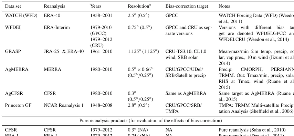
Table 9. Historical climate forcing data sets for Phase 1.
Data set Reanalysis Years Resolution∗ Bias-correction target Notes
WATCH (WFD) ERA-40 1958–2001 2.5◦(0.5◦) GPCC WATCH Forcing Data (WFD) (Weedon
et al., 2011)
WFDEI ERA-Interim 1979-2010
(GPCC) 1979–2012 (CRU)
0.75◦(0.5◦) GPCC and CRU as
sep-arate versions
Versions with different bias
tar-get are denoted WFDEI.GPCC and WFDEI.CRU (Weedon et al., 2014)
GRASP JRA-25 & ERA-40 1961–2010 1.125◦(1.125◦) CRU-TS3.10, CL1.0
wind, SRB solar
Mean/max/min 2 m temp, precip, so-lar, vap pres., 10 m wind (Iizumi et al., 2014)
AgMERRA MERRA 1980–2010 0.5◦×0.66◦
(0.5◦/0.25◦)
CRU/GPCC/UDel/ SRB/Satellite precip
Precip: CMORPH, PERSIANN,
TRMM. Out: Tmax/min, precip, solar, RHS at Tmax, wind (Ruane et al., 2015)
AgCFSR CFSR 1980–2010 0.3◦
(0.5◦/0.25◦)
Same as AgMERRA Same target as AgMERRA (Ruane et
al., 2015)
Princeton GF NCAR Reanalysis 1 1948–2008 2.8◦(0.5◦) CRU/GPCC/SRB/
TMPA
TMPA: TRMM Multi-satellite Precipi-tation Analysis (Sheffield et al., 2006)
Pure reanalysis products (for evaluation of the effects of bias-correction)
CFSR CFSR 1979–2012 0.3◦(NA) NA Pure reanalysis (Saha et al., 2010)
ERA-I ERA-I 1979–2012 0.75◦(NA) NA Pure reanalysis (Dee et al., 2011)
∗This denotes the resolution of the underlying reanalysis data set (and in parentheses the typical resolution of the key target data, temperature, and precipitation, used in the bias-correction). All
data sets will be standardized to a 0.5×0.5◦spatial resolution in the GGCMI archives.
for each crop type and cover current crop-specific growing areas, up to 473 units for the maize nitrogen fertilizer data (Mueller et al., 2012). Therefore we harmonized the admin-istrative boundary units across crop and nutrient types for the interpolation procedure here. Data on manure application (Potter et al., 2010) have resolution finer than political units, as they are based off a gridded livestock data set. Thus, the manure nutrient maps were simply aggregated to each of the 372 administrative units as an area-weighted average.
In a third step, we harmonized the reference units between organic and inorganic fertilizers (manure). Original manure data are reported in terms of atomic nitrogen (N) and phos-phorus (P) and assumed to contain no potassium (Potter et al., 2010), whereas inorganic fertilizer data are reported as N, phosphate (P2O5), and potassium oxide (K2O). The
con-version from P manure to P2O5is based on atomic masses
P2O5−eq.=P/31×(31×2+5×16). (1)
Nutrients from manure are generally less available to plants than mineral fertilizers. We assume 60 % of applied N-manure and 75 % of applied P-manure to be plant avail-able (Rosen and Bierman, 2005).
In the final step, we extrapolated fertilizer application rates to currently uncultivated land. The original data on mineral fertilizers (Mueller et al., 2012) cover only crop-specific harvested areas. First, we assigned the national aver-age nutrient-specific fertilizer rate (area-weighted) to all ad-ministrative units that do not apply any mineral fertilizer or manure in the original data but are within a country that does reporting fertilizer application. Second, for all other
coun-tries that do not currently apply fertilizer to grow the spe-cific crop, we attributed estimated nutrient-spespe-cific applica-tion rates by averaging fertilizer applicaapplica-tion rates over the corresponding income level group. We base income level groups on the World Bank’s definition to classify countries by income level: economies are divided according to 2012 gross national income per capita, calculated using the World Bank Atlas method5. The groups are as follows: low income, USD 1035 or less; lower middle income, USD 1036–4085; upper middle income, USD 4086–12 615; and high income, USD 12 616 or more. We averaged fertilizer application rates for all countries with fertilizer applications of larger than zero within the income level group and applied those rates to all countries without fertilizer data within that group. 3.3.2 Implementation instructions
All fertilizer data supplied here should be treated as mineral fertilizer; organic fertilizer (manure) has been reduced to ac-count for limited plant availability and combined with data on inorganic fertilizer applications.
3.4 Other data and parameter recommendations
In addition to management drivers, we harmonize historical CO2levels based on the Mauna Loa Observatory time series
(Thoning et al., 1989). We also provide instructions for how to measure growing seasons, and provide guidance on
T able 10. W eather v ariables supplied per data set. V ariable long name Unit W A TCH WFDEI GRASP AgMERRA AgCFSR PGF CFSR ERA-I Notes tas daily mean temperature ◦ C x x x x x x x x tasmin daily min. temperature ◦ C x x x x x x x x tasmax daily max. temperature ◦ C x x x x x x x x pr daily avg. precip. flux rate kg m − 2 s− 1 x 1 gpcc(’10) 1 cru(’12) 1 x x x x x x (incl. sno w) rsds short w av e do wnw ard W m − 2 x x x x x x x x rlds long w av e do wnw ard W m − 2 x x N A N A N A x x x wind wind speed m s− 1 x x x x x x x x hur relati v e humidity % x x x at Tmax & T avg at Tmax & T avg * x * hus specific humidity kg kg − 1 x x N A N A N A x N A x v ap v apor pressure P a * * x * * * * * ps surf ace pressure P a x x N A N A N A x N A x x – These v ariables are directly pro vided by the climate data pro vider . * – These v ariables are not directly pro vided b ut can be calculated using standard relationships (Bolton, 1980) which we implement in GGCMI. N A – These v ariables are not av ailable from the gi v en data set. 1 – W A TCH and WFDEI pro vide rainf all and sno wf all separately . In the final v ersion of the data set used for GGCMI, these ha v e been combined.
1950 1970 1990 2010
500
600
700
800
rain-fed wheat area
year
ann
ual mean precipitation [mm]
A
1950 1970 1990 2010
1400
1800
2200
2600
rain-fed rice area
year
ann
ual mean precipitation [mm]
B
1950 1970 1990 2010
800
1000
1200
1400
rain-fed maize area
year
ann
ual mean precipitation [mm]
C
1950 1970 1990 2010
900
1100
1300
rain-fed soy area
year
ann
ual mean precipitation [mm]
D WATCH WFDEI.CRU WFDEI.GPCC AgMERRA AgCFSR Princeton GRASP ERAI CFSR
Figure 2. Area-weighted mean of annual precipitation [◦C] for cropping areas for rain-fed wheat (a), rice (b), maize (c), and soy (d).
rameter choices for automatic irrigation algorithms (where applicable).
3.5 Data format conventions of input data
All input data are supplied in gridded format at 0.5◦×0.5◦ spatial resolution in a compressed NetCDF4 file format. Weather data are available at daily time steps and at 3-hourly values for WFDEI (which is required for some participat-ing land-surface models). Management data are available for only one time period and are assumed to apply for all his-toric time periods since data are lacking in changes in man-agement over time (all comparisons are done between de-trended observation and simulation time series, which greatly reduces, but certainly does not eliminate the effect of changes in management practices and technology over time).
4 Evaluation data sets and procedures 4.1 Historical yield data
Table 11. Combination of crop calendar data in GGCMI data sets.
GGCMI crop MIRCA2000 SAGE LPJmL Days maturity to harvest
Barley Barley Barley spring+winter Wheat 7a
Cassava Cassava Cassava Cassava Assuming 0b
Groundnuts Groundnuts Groundnuts Groundnuts 0c
Maize Maize Maize Maize 1–28d, here 21
Millet Millet Millet Millet Assuming 0
Potatoes Potatoes Potatoes Sugar beets Assuming 0
Pulses (dry bean, field peas)
Pulses Pulses Pulses Assuming 0
Rapeseed Rapeseed Rapeseed, winter Rapeseed Same as wheat=7
Rice Rice Rice Rice 0eor 8–12f, herea
Rye Rye Rye, winter Wheat 7a
Sorghum Sorghum Sorghum Millet 0g
Soybeans Soybeans Soybeans Soybeans 7–21hhere 21
Sugar beets Sugar beets Sugar beets Sugar beets Assuming 0
Sugarcane Sugarcane NA Sugarcane Assuming 0
Sunflower Sunflower Sunflower Sunflower 0i
Wheat Wheat Wheat, spring+winter Wheat 3jto 8k, here 7
aAssuming quick harvests for barley, rice, rye, and wheat as they are all threatened by pre-harvest sprouting (see, e.g.,
http://www.dpi.nsw.gov.au/data/assets/pdf_file/0010/445636/farrer_oration_1981_nf_derera.pdf) but allowing some time to dry after full maturity.bCan be anything from 0 days to up to 6 months, harvest on demand.
chttp://www.interaide.org/pratiques_old/pages/agro/3cultures/Phalombe_Mlwi_crop_management_2010.pdf, p. 8.
dhttp://www.smartgardener.com/plants/4159-corn-cherokee-white-flour/harvesting.
ehttp://agris.fao.org/agris-search/search/display.do?f=19902FPH3FPH90013.xml3BPH8811720.
fhttp://www.interaide.org/pratiques_old/pages/agro/3cultures/Phalombe_Mlwi_crop_management_2010.pdf, p. 13. ghttp://www.interaide.org/pratiques_old/pages/agro/3cultures/Phalombe_Mlwi_crop_management_2010.pdf, p. 14. hhttp://agris.fao.org/agris-search/search/display.do?f=20092FJP2FJP0932.xml3BJP2009005739.
ihttp://www.interaide.org/pratiques_old/pages/agro/3cultures/Phalombe_Mlwi_crop_management_2010.pdf, p. 12.
jhttp://agris.fao.org/agris-search/search/display.do?f=20092FJP2FJP0938.xml3BJP2009007527.khttp://www.dwd.de/bvbw/appmanager/bvbw/
dwdwwwDesktop?_nfpb=true_windowLabel=T94008&_urlType=action&_pageLabel=dwdwww_klima_umwelt_phaenologie shows that there are 16 days between “hard dough” stage (BBCH87) and harvest in Germany, and http://www.dwd.de/bvbw/generator/DWDWWW/Content/Landwirtschaft/Dokumentation/ AgroProg/Kornfeuchte,templateId=raw,property=publicationFile.pdf/Kornfeuchte.pdf shows that there are about 8 days between “hard dough” and “fully ripe” (BBCH89) stages, so that the difference between “fully ripe” and harvest is 8 days as well.
sub-national, and sub-subnational statistics, spanning 1961– 2008, and provided at a nominal resolution of 5 arc minutes by distributing yield statistics from administrative units to grid cells evenly based on the approximate distribution of crop areas in the unit, without any proxy measurements of the relative distribution of attained yields. To fill in the gaps for crops and years that are not available in these first two data sets, we will compare aggregated simulation outputs at the national level directly with statistics from FAOSTAT.
4.2 Open-source processing and evaluation pipeline
In order to ensure consistency and encourage consensus in GGCMI products, we are developing all output processing software utilities within an open software repository avail-able at https://github.com/RDCEP/ggcmi/. Additionally, we permanently archive the intermediate and final results of each step in the output processing pipeline on the GGCMI data servers. These data will be made available along with the data supplied by GGCMI modeling groups at the time of pub-lic release. The key stages of the pipeline are described in Sects. 4.2.1–4.2.4.
Figure 3. N-equivalent application rate of nitrogen fertilizers for the production of wheat.
4.2.1 Aggregation
All simulated data are first aggregated up to administra-tive and environmental boundaries, including state/province (GADM6level 1), country (GADM level 0), river basins and
food producing units (FPUs; river basins crossed with
A) Wheat Yield – Iizumi et al. 2013 (t/ha) B) Wheat Yield – Ray et al. 2012 (t/ha)
Figure 4. Example of historical evaluation data for year 2000 wheat yields from (a) Iizumi et al. (2013) (at 1.125◦spatial resolution) and (b) Ray et al. (2012) (aggregated from 5 arc minutes to 0.5◦).
Figure 5. Example of a global Köppen–Geiger climate classifica-tion.
tries (Cai and Rosegrant, 2002)), Köppen–Geiger climate re-gions (Peel et al., 2007) (example shown in Fig. 5), and large-scale continental or sub-continental regions.
4.2.2 De-trending
In order to compare FAOSTAT observations with simulation results, we must remove trends from the statistics. As there are several methods to remove trends from observed data and no one method works best in all situations, we employ four distinct de-trending methods: we take (i) the linear or (ii) quadratic trends from a least squares regression (Fig. 6, right), (iii) we take a 7-year moving mean trend, and (iv) we calculate the fraction first differences,Yt/Yt−1−1, of the
se-ries and remove a linear trend (Fig. 6, right). All conclusions and results are then checked for robustness against all the de-trending method used.
4.2.3 Multi-metric evaluation
GGCMI uses a varied approach to evaluate model outputs over the evaluation period, comparing reference data and simulations using a number of metrics and methodologies. In preliminary analysis, metrics evaluated include the time series correlation, root mean square error, ratio of simulated
and observed coefficients of variation, and the top and bot-tom hit rates (number of years in the top and botbot-tom quintile of the observation series that are reproduced in the simulated series). The metrics are formalized in the output processing pipeline in a set of multi-dimensional metric files, which are provided along with a plotting application that produces two-dimensional cross sections by selecting, averaging, or opti-mizing over any combination of dimensions (an example ar-ray is shown in Fig. 7).
4.2.4 Multi-model ensembles
In the final processing step, we aim to produce multi-model ensemble versions of the output to evaluate, for example, how well the ensemble performs relative to individual mod-els, highlighting individual model skill and deficiencies vs. model community skills and deficiencies. This step uses the multi-metric files to produce versions of the simulated vari-ables that aggregate all of the models into various combina-tions. Ensembles range in complexity from simple averages (all models weighted equally) to weighted averages using one or more evaluation metric, and from all models included in the average to the inclusion of only the top-performing model. Finally, we produce evaluation multi-metric files for the ensemble combinations to easily facilitate comparison of the ensemble measurements with individual models. This will be the basis for identifying central processes in models that are responsible for differences in model performance as well as general model deficiencies that require improvements in all models and in understanding. This phase will likely re-quire additional simulations with modified models.
5 GGCMI data archive and crediting
1960 1970 1980 1990 2000 2010
2 3 4 5 6 7
8 Historical Maize Yieldtha
1970 1980 1990 2000 2010
0.2 0.0 0.2 0.4
Historical Maize YieldFractional First Difference A) Historical Maize Yield (t/ha) B) Historical Maize Yield (fractional first difference)
Figure 6. (a) FAOSTAT yield for maize in Argentina (solid line and points) with the linear (blue) and quadratic (red) best-fits and 7-year moving average (gray). (b) Fractional first difference of maize yields in Argentina (gray), the linear trend (blue line) and the fractional first difference with the trend removed (red).
A
B
Figure 7. Examples of cross sections of the multi-metric evaluation array for the top two maize-producing countries – the United States (a) and China (b). Plot shows time series correlations for eight different crop models run (xaxis) with nine different climate forcing data sets (yaxis). For each model/climate combination, the best metric value among the scenarios (default, fullharm, and harmnon) and de-trending methods (linear, quadratic, moving mean, and trend-removed fraction first difference) are shown.
ties, for example, through engagement processes established as part of frequent regional and global workshops hosted by AgMIP, to improve archive access and usability. During each phase of the project (i.e., before the public launch of the re-sulting archive), all inputs and outputs generated belong to the GGCMI as a team (i.e., all GGCMI modelers) and must not be used, distributed, presented, or published in any indi-vidual or selected study without the consent of the group of contributing GGCMI modelers. During this time, presenta-tions and publicapresenta-tions will be led by GGCMI team members and will be coordinated through the GGCMI coordinators. The publications must acknowledge each individual contri-bution, including providers of not publicly available input or reference data, via co-authorship or other agreed acknowl-edgement.
Because GGCMI acts as the sectoral coordinator for crop modeling in Phase 2 of the ISI-MIP project (ISI-MIP2), we have designed the GGCMI protocols to overlap with (planned) ISI-MIP2 simulations as closely as possible. Upon the data submission deadline as defined by ISI-MIP2,
GGCMI data will automatically be transferred to ISI-MIP2, unless otherwise specified by participating modelers. At this time, GGCMI modelers become ISI-MIP2 participants and additional restrictions or specifications for data availability, as negotiated between ISI-MIP2 and GGCMI coordinators and modelers, may apply at this time.
6 Discussion
al., 2014; Elliott et al., 2014a; Nelson et al., 2014), the bring-ing together of modelers workbring-ing independently on com-plex dynamic phenomena to compare and synthesize out-puts can generate substantive insights and innovations that are not generally possible otherwise. A key observation from the AgMIP/ISI-MIP Fast Track and other recent model inter-comparisons (Rosenzweig et al., 2014; Nelson et al., 2014; Challinor et al., 2014), and a key motivation for GGCMI, is the importance of harmonization of input data and assump-tions.
Each phase of GGCMI will include planning, simula-tion, analysis, and publication components that will build on the inputs, science, and deliverables of the previous phase. In Phase 2, GGCMI participants will conduct a multi-dimensional sensitivity study of model response to carbon dioxide, temperature, water, and nitrogen (CTWN) organized around a set of simulations driven by perturbed versions of the historical and harmonized data products prepared in Phase 1. Results will be used both to analyze model sensi-tivity and to develop high-resolution multi-dimensional re-sponse surfaces that can be aggregated into arbitrary ad-ministrative or environmental boundaries and will be tested for suitability as efficient multi-model emulators. In Phase 3, GGCMI participants will conduct a comprehensive as-sessment of climate vulnerabilities, impacts, and adaptations using a new set of future climate forcings from CMIP5 and Coordinated Regional Climate Downscaling Experiment (CORDEX) and a detailed set of adaptation scenarios de-veloped in the AgMIP Representative Agricultural Path-ways (RAPs) framework. GGCMI also builds on other exist-ing AgMIP projects, such as the Coordinated Climate-Crop Modeling Project (Ruane et al., 2014), and cross-cutting themes such as uncertainty and spatial scaling/aggregation.
During GGCMI’s 3-year duration, our aim is for the com-munity to create a new standard for research on global change vulnerabilities, impacts, and potential adaptations. Data products, analyses and insights are to be published in peer-reviewed scientific journals and will thus be accessible to the scientific community. Due to the open and accessi-ble structure of the project and its data distribution archi-tecture, we expect important scientific outcomes and deliv-erables to evolve and develop during and well beyond the planned project lifetime. GGCMI leverages and relies on the contributions of many partners that typically lack funding for this project. However, the tremendous enthusiasm that this project has generated among participants and user communi-ties makes us confident that GGCMI will succeed in accom-plishing its stated goals – and, with high likelihood, greatly surpass those goals. In addition, close partnership with the AgMIP and ISI-MIP networks and the active participation of leaders from those groups, will help ensure that GGCMI is highly visible within and beyond the scientific community. The GGCMI team will also work with potential end users to facilitate usage of GGCMI results downstream in economic models and globally and regionally integrated assessments.
For this purpose we are developing several use cases for the existing Fast Track archive (Nelson et al., 2014) and work-ing with economic modelwork-ing communities such as the En-ergy Modeling Forum (EMF) and the Global Trade Analysis Project (GTAP)7 and actively seek funding for GGCMI ac-tivities and cooperation with other groups.
The standardized, protocol-based model intercomparison described here will be the basis for a clear analysis of model skills and deficiencies, identification and reduction of crop model uncertainties, and identification of future development paths to improve models and assessments. Clearly, more work than is envisioned here is needed in analyzing and im-proving crop modeling skills for gridded large-scale appli-cations. Still, the first phase of GGCMI will provide a solid basis for future work by providing not only standardized in-puts and reference data but also open-access data processing and analysis tools. During this first part of the project, by identifying the main sources of uncertainty and model dis-agreement, we expect that key conditions for the next phase of analysis will take shape. We hope to support all large-scale crop modeling efforts with the insights and analysis tools that are produced in GGCMI, and we invite all agricultural scien-tists to contribute to the development and framing of the next phases of the project and protocols.
Acknowledgements. J. Elliott acknowledges financial support from
the National Science Foundation under grants SBE-0951576 and GEO-1215910. C. Müller acknowledges financial support from the KULUNDA project (01LL0905L) and the FACCE MACSUR project (031A103B) funded through the German Federal Ministry of Education and Research (BMBF). Computing and data resources provided through the University of Chicago Research Computing Center.
Edited by: A. B. Guenther
References
Asseng, S., Ewert, F., Rosenzweig, C., Jones, J. W., Hatfield, J. L., Ruane, A. C., Boote, K. J., Thorburn, P. J., Rotter, R. P., Cam-marano, D., Brisson, N., Basso, B., Martre, P., Aggarwal, P. K., Angulo, C., Bertuzzi, P., Biernath, C., Challinor, A. J., Doltra, J., Gayler, S., Goldberg, R., Grant, R., Heng, L., Hooker, J., Hunt, L. A., Ingwersen, J., Izaurralde, R. C., Kersebaum, K. C., Müller, C., Naresh Kumar, S., Nendel, C., O/’Leary, G., Olesen, J. E., Osborne, T. M., Palosuo, T., Priesack, E., Ripoche, D., Semenov, M. A., Shcherbak, I., Steduto, P., Stockle, C., Stratonovitch, P., Streck, T., Supit, I., Tao, F., Travasso, M., Waha, K., Wallach, D., White, J. W., Williams, J. R., and Wolf, J.: Uncertainty in simu-lating wheat yields under climate change, Nat. Clim. Change, 3, 827–832, doi:10.1038/NCLIMATE1916, 2013.
Balkoviˇc, J., van der Velde, M., Schmid, E., Skalský, R., Khabarov, N., Obersteiner, M., Stürmer, B., and Xiong, W.: Pan-European
crop modelling with EPIC: Implementation, up-scaling and re-gional crop yield validation, Agricultural Systems, 120, 61–75, doi:10.1016/j.agsy.2013.05.008, 2013.
Bolton, D.: The Computation of Equivalent Potential Tempera-ture, Mon. Weather Rev., 108, 1046–1053, doi:10.1175/1520-0493(1980)108<1046:TCOEPT>2.0.CO;2, 1980.
Bondeau, A., Smith, P. C., Zaehle, S., Schaphoff, S., Lucht, W., Cramer, W., Gerten, D., Lotze-Campen, H., Müller, C., Reichstein, M., and Smith, B.: Modelling the role of agri-culture for the 20th century global terrestrial carbon bal-ance, Glob. Change Biol., 13, 679–706, doi:10.1111/j.1365-2486.2006.01305.x, 2007.
Cai, X. M. and Rosegrant, M. W.: Global water demand and supply projections part – 1. A modeling approach, Water Int., 27, 159– 169, 2002.
Challinor, A. J., Wheeler, T. R., Craufurd, P. Q., Slingo, J. M., and Grimes, D. I. F.: Design and optimisation of a large-area process-based model for annual crops, Agr. Forest Meteorol., 124, 99– 120, 2004.
Challinor, A. J., Watson, J., Lobell, D. B., Howden, S. M., Smith, D. R., and Chhetri, N.: A meta-analysis of crop yield under cli-mate change and adaptation, Nat. Clim. Change, 4, 287–291, doi:10.1038/nclimate2153, 2014.
Dee, D. P., Uppala, S. M., Simmons, A. J., Berrisford, P., Poli, P., Kobayashi, S., Andrae, U., Balmaseda, M. A., Balsamo, G., Bauer, P., Bechtold, P., Beljaars, A. C. M., van de Berg, L., Bid-lot, J., Bormann, N., Delsol, C., Dragani, R., Fuentes, M., Geer, A. J., Haimberger, L., Healy, S. B., Hersbach, H., Hólm, E. V., Isaksen, L., Kållberg, P., Köhler, M., Matricardi, M., McNally, A. P., Monge-Sanz, B. M., Morcrette, J. J., Park, B. K., Peubey, C., de Rosnay, P., Tavolato, C., Thépaut, J. N., and Vitart, F.: The ERA-Interim reanalysis: configuration and performance of the data assimilation system, Q. J. Roy. Meteorol. Soc., 137, 553– 597, doi:10.1002/qj.828, 2011.
de Noblet-Ducoudre, N., Gervois, S., Ciais, P., Viovy, N., Brisson, N., Seguin, B., and Perrier, A.: Coupling the Soil-Vegetation-Atmosphere-Transfer Scheme ORCHIDEE to the agronomy model STICS to study the influence of croplands on the Euro-pean carbon and water budgets, Agronomie, 24, 397–407, 2004. Deryng, D., Sacks, W. J., Barford, C. C., and Ramankutty, N.: Sim-ulating the effects of climate and agricultural management prac-tices on global crop yield, Global Biogeochem. Cy., 25, GB2006, doi:10.1029/2009GB003765, 2011.
Deryng, D., Conway, D., Ramankutty, N., Price, J., and Warren, R.: Global crop yield response to extreme heat stress under mul-tiple climate change futures, Environ. Res. Lett., 9, 034011, doi:10.1088/1748-9326/9/3/034011, 2014.
Drewniak, B., Song, J., Prell, J., Kotamarthi, V. R., and Jacob, R.: Modeling agriculture in the Community Land Model, Geosci. Model Dev., 6, 495–515, doi:10.5194/gmd-6-495-2013, 2013. Elliott, J., Deryng, D., Müller, C., Frieler, K., Konzmann, M.,
Gerten, D., Glotter, M., Flörke, M., Wada, Y., Best, N., Eis-ner, S., Fekete, B. M., Folberth, C., Foster, I., Gosling, S. N., Haddeland, I., Khabarov, N., Ludwig, F., Masaki, Y., Olin, S., Rosenzweig, C., Ruane, A. C., Satoh, Y., Schmid, E., Stacke, T., Tang, Q., and Wisser, D.: Constraints and potentials of future irrigation water availability on agricultural production under climate change, P. Natl. Acad. Sci., 111, 3239–3244, doi:10.1073/pnas.1222474110, 2014a.
Elliott, J., Kelly, D., Chryssanthacopoulos, J., Glotter, M., Jhunjh-nuwala, K., Best, N., Wilde, M., and Foster, I.: The parallel sys-tem for integrating impact models and sectors, Environ. Model. Softw., 62, 509–516, doi:10.1016/j.envsoft.2014.04.008, online first, 2014b.
FAOSTAT data: available at: http://faostat.fao.org/ (last access: 1 November 2013), 2013.
Foley, J. A., Ramankutty, N., Brauman, K. A., Cassidy, E. S., Ger-ber, J. S., Johnston, M., Mueller, N. D., O’Connell, C., Ray, D. K., West, P. C., Balzer, C., Bennett, E. M., Carpenter, S. R., Hill, J., Monfreda, C., Polasky, S., Rockstrom, J., Sheehan, J., Siebert, S., Tilman, D., and Zaks, D. P. M.: Solutions for a cultivated planet, Nature, 478, 337–342, doi:10.1038/nature10452, 2011. Gueneau, A., Schlosser, C. A., Strzepek, K. M., Gao, X., and
Monier, E.: CLM-AG: An Agriculture Module for the Commu-nity Land Model version 3.5, MIT Joint Program on the Science and Policy of Global Change, 2012.
Iizumi, T., Yokozawa, M., Sakurai, G., Travasso, M. I., Ro-manernkov, V., Oettli, P., Newby, T., Ishigooka, Y., and Fu-ruya, J.: Historical changes in global yields: major cereal and legume crops from 1982 to 2006, Global Ecol. Biogeogr., doi:10.1111/geb.12120, online first, 2013.
Iizumi, T., Yokozawa, M., Sakurai, G., Travasso, M. I., Roman-ernkov, V., Oettli, P., Newby, T., Ishigooka, Y., and Furuya, J.: Historical changes in global yields: major cereal and legume crops from 1982 to 2006, Global Ecol. Biogeogr., 23, 346–357, doi:10.1111/geb.12120, 2014.
Izaurralde, R. C., Williams, J. R., McGill, W. B., Rosenberg, N. J., and Jakas, M. C. Q.: Simulating soil C dynamics with EPIC: Model description and testing against long-term data, Ecol. Model., 192, 362–384, 2006.
Jones, J. W., Hoogenboom, G., Porter, C. H., Boote, K. J., Batchelor, W. D., Hunt, L. A., Wilkens, P. W., Singh, U., Gijsman, A. J., and Ritchie, J. T.: The DSSAT cropping system model, Eur. J. Agron., 18, 235–265, 2003.
Keating, B. A., Carberry, P. S., Hammer, G. L., Probert, M. E., Robertson, M. J., Holzworth, D., Huth, N. I., Hargreaves, J. N. G., Meinke, H., Hochman, Z., McLean, G., Verburg, K., Snow, V., Dimes, J. P., Silburn, M., Wang, E., Brown, S., Bristow, K. L., Asseng, S., Chapman, S., McCown, R. L., Freebairn, D. M., and Smith, C. J.: An overview of APSIM, a model designed for farming systems simulation, Eur. J. Agron., 18, 267–288, doi:10.1016/S1161-0301(02)00108-9, 2003.
Levis, S., Bonan, G. B., Kluzek, E., Thornton, P. E., Jones, A., Sacks, W. J., and Kucharik, C. J.: Interactive Crop Manage-ment in the Community Earth System Model (CESM1): Seasonal Influences on Land-Atmosphere Fluxes, J. Climate, 25, 4839– 4859, doi:10.1175/JCLI-D-11-00446.1, 2012.
Lindeskog, M., Arneth, A., Bondeau, A., Waha, K., Seaquist, J., Olin, S., and Smith, B.: Implications of accounting for land use in simulations of ecosystem carbon cycling in Africa, Earth Syst. Dynam., 4, 385–407, doi:10.5194/esd-4-385-2013, 2013. Liu, J. G., Williams, J. R., Zehnder, A. J. B., and Yang, H.:
GEPIC – modelling wheat yield and crop water productivity with high resolution on a global scale, Agr. Syst., 94, 478–493, doi:10.1016/j.agsy.2006.11.019, 2007.
nutrient and water management, Nature, 490, 254–257, doi:10.1038/nature11420, 2012.
Müller, C. and Robertson, R.: Projecting future crop productiv-ity for global economic modeling, Agric. Econom., 45, 37–50, doi:10.1111/agec.12088, 2014.
Nelson, G. C., Valin, H., Sands, R. D., Havlík, P., Ahammad, H., Deryng, D., Elliott, J., Fujimori, S., Hasegawa, T., Heyhoe, E., Kyle, P., Von Lampe, M., Lotze-Campen, H., Mason d’Croz, D., van Meijl, H., van der Mensbrugghe, D., Müller, C., Popp, A., Robertson, R., Robinson, S., Schmid, E., Schmitz, C., Tabeau, A., and Willenbockel, D.: Climate change effects on agriculture: Economic responses to biophysical shocks, P. Natl. Acad. Sci., 111, 3274–3279, 10.1073/pnas.1222465110, 2014.
Okada, M., Iizumi, T., Hayashi, Y., and Yokozawa, M.: Mod-eling the multiple effects of temperature and radiation on rice quality, Environ. Res. Lett., 6, 034031, doi:10.1088/1748-9326/6/3/034031, 2011.
Peel, M. C., Finlayson, B. L., and McMahon, T. A.: Updated world map of the Köppen–Geiger climate classification, Hy-drol. Earth Syst. Sci., 11, 1633–1644, doi:10.5194/hess-11-1633-2007, 2007.
Piontek, F., Müller, C., Pugh, T. A. M., Clark, D. B., Deryng, D., Elliott, J., Colón González, F. d. J., Flörke, M., Folberth, C., Franssen, W., Frieler, K., Friend, A. D., Gosling, S. N., Hem-ming, D., Khabarov, N., Kim, H., Lomas, M. R., Masaki, Y., Mengel, M., Morse, A., Neumann, K., Nishina, K., Ostberg, S., Pavlick, R., Ruane, A. C., Schewe, J., Schmid, E., Stacke, T., Tang, Q., Tessler, Z. D., Tompkins, A. M., Warszawski, L., Wisser, D., and Schellnhuber, H. J.: Multisectoral climate im-pact hotspots in a warming world, P. Natl. Acad. Sci., 111, 3233– 3238, doi:10.1073/pnas.1222471110, 2014.
Portmann, F. T., Siebert, S., Bauer, C., and Döll, P.: Global data set of monthly growing areas of 26 irrigated crops, Institute of Physical Geography, University of Frankfurt, Frankfurt am Main, GermanyFrankfurt Hydrology Paper 06, 400, 2008.
Portmann, F. T., Siebert, S., and Döll, P.: MIRCA2000-Global monthly irrigated and rainfed crop areas around the year 2000: A new high-resolution data set for agricultural and hy-drological modeling, Global Biogeochem. Cy., 24, Gb1011, doi:10.1029/2008gb003435, 2010.
Potter, P., Ramankutty, N., Bennett, E. M., and Donner, S. D.: Characterizing the Spatial Patterns of Global Fertilizer Appli-cation and Manure Production, Earth Interactions, 14, 1–22, doi:10.1175/2009EI288.1, 2010.
Ray, D. K., Ramankutty, N., Mueller, N. D., West, P. C., and Foley, J. A.: Recent patterns of crop yield growth and stagnation, Nat. Commun., 3, 1293, doi:10.1038/ncomms2296, 2012.
Ray, D. K., Mueller, N. D., West, P. C., and Foley, J. A.: Yield Trends Are Insufficient to Double Global Crop Production by 2050, Plos One, 8, e66428, doi:10.1371/journal.pone.0066428, 2013.
Rosen, C. J. and Bierman, P. M.: Using manure and compost as nutrient sources for fruit and vegetable crops, Publication of the Department of Soil, Water, and Climate University of Minnesota, 2005.
Rosenzweig, C., Jones, J. W., Hatfield, J. L., Ruane, A. C., Boote, K. J., Thorburne, P., Antle, J. M., Nelson, G. C., Porter, C., Janssen, S., Asseng, S., Basso, B., Ewert, F., Wal-lach, D., Baigorria, G., and Winter, J. M.: The Agricultural
Model Intercomparison and Improvement Project (AgMIP): Pro-tocols and pilot studies, Agr. Forest Meteorol., 170, 166–182, doi:10.1016/j.agrformet.2012.09.011, 2013.
Rosenzweig, C., Elliott, J., Deryng, D., Ruane, A. C., Müller, C., Arneth, A., Boote, K. J., Folberth, C., Glotter, M., Khabarov, N., Neumann, K., Piontek, F., Pugh, T. A. M., Schmid, E., Ste-hfest, E., Yang, H., and Jones, J. W.: Assessing agricultural risks of climate change in the 21st century in a global gridded crop model intercomparison, P. Natl. Acad. Sci., 111, 3268–3273, doi:10.1073/pnas.1222463110, 2014.
Ruane, A. C., McDermid, S., Rosenzweig, C., Baigorria, G. A., Jones, J. W., Romero, C. C., and DeWayne Cecil, L.: Carbon– Temperature–Water change analysis for peanut production under climate change: a prototype for the AgMIP Coordinated Climate-Crop Modeling Project (C3MP), Glob. Change Biol., 20, 394– 407, doi:10.1111/gcb.12412, 2014.
Ruane, A. C., Goldberg, R., and Chryssanthacopoulos, J.: Climate forcing datasets for agricultural modeling: Merged products for gap-filling and historical climate series estimation, Agr. Forest Meteorol., 200, 233–248, doi:10.1016/j.agrformet.2014.09.016, 2015.
Sacks, W. J., Deryng, D., Foley, J. A., and Ramankutty, N.: Crop planting dates: an analysis of global patterns, Global Ecol. Biogeogr., 19, 607–620, doi:10.1111/j.1466-8238.2010.00551.x, 2010.
Saha, S., Moorthi, S., Pan, H.-L., Wu, X., Wang, J., Nadiga, S., Tripp, P., Kistler, R., Woollen, J., Behringer, D., Liu, H., Stokes, D., Grumbine, R., Gayno, G., Wang, J., Hou, Y.-T., Chuang, H.-Y., Juang, H.-M. H., Sela, J., Iredell, M., Treadon, R., Kleist, D., Van Delst, P., Keyser, D., Derber, J., Ek, M., Meng, J., Wei, H., Yang, R., Lord, S., Van Den Dool, H., Kumar, A., Wang, W., Long, C., Chelliah, M., Xue, Y., Huang, B., Schemm, J.-K., Ebisuzaki, W., Lin, R., Xie, P., Chen, M., Zhou, S., Higgins, W., Zou, C.-Z., Liu, Q., Chen, Y., Han, Y., Cucurull, L., Reynolds, R. W., Rutledge, G., and Goldberg, M.: The NCEP Climate Fore-cast System Reanalysis, B. Am. Meteorol. Soc., 91, 1015–1057, doi:10.1175/2010BAMS3001.1, 2010.
Sheffield, J., Goteti, G., and Wood, E. F.: Development of a 50-Year High-Resolution Global Dataset of Meteorological Forc-ings for Land Surface Modeling, J. Climate, 19, 3088–3111, doi:10.1175/JCLI3790.1, 2006.
Smith, B., Prentice, I. C., and Sykes, M. T.: Representation of vegetation dynamics in the modelling of terrestrial ecosystems: comparing two contrasting approaches within European climate space, Global Ecol. Biogeogr., 10, 621–637, 2001.
Song, Y., Jain, A. K., and McIsaac, G. F.: Implementation of dy-namic crop growth processes into a land surface model: eval-uation of energy, water and carbon fluxes under corn and soy-bean rotation, Biogeosciences, 10, 8039–8066, doi:10.5194/bg-10-8039-2013, 2013.
Stehfest, E., Heistermann, M., Priess, J. A., Ojima, D. S., and Alcamo, J.: Simulation of global crop production with the ecosystem model DayCent, Ecol. Model., 209, 203–219, doi:10.1016/j.ecolmodel.2007.06.028, 2007.
Stöckle, C. O., Donatelli, M., and Nelson, R.: CropSyst, a crop-ping systems simulation model, Eur. J. Agron., 18, 289–307, doi:10.1016/S1161-0301(02)00109-0, 2003.
![Figure 2. Area-weighted mean of annual precipitation [◦C] forcropping areas for rain-fed wheat (a), rice (b), maize (c), and soy(d).](https://thumb-us.123doks.com/thumbv2/123dok_us/9065167.1899012/10.612.92.240.70.704/figure-weighted-annual-precipitation-forcropping-areas-wheat-maize.webp)