Vol. 5, No. 3, 2013 Article ID IJIM-00239, 10 pages Research Article
New iterative method for solving linear Fredholm fuzzy integral
equations of the second kind
A. Jafarian ∗ † , S. Measoomy Nia ‡
————————————————————————————————–
Abstract
Fuzzy integral equations play major roles in various areas, therefore a new method for finding a solution of the Fredholm fuzzy integral equation is presented. This method converts the fuzzy integral equation into linear system by using the Taylor series. For this scope, first the Taylor expansion of unknown function is substituted in parametric form of the given equation. Then we differentiate both sides of the resulting integral equation and also approximate the Taylor expansion by a suitable truncation limit. This work yields a linear system in crisp case. Now the solution of this system yields unknown Taylor coefficients of the solution functions. The proposed method is illustrated by several examples with computer simulations.
Keywords : Fredholm fuzzy integral equations; Taylor series; Convergence analysis; Approximate solutions.
—————————————————————————————————–
1
Introduction
S
ince many mathematical formulations of phys-ical phenomena contain fuzzy integral equa-tions and these equaequa-tions are very useful for solv-ing many problems in several applied fields like mathematical physics and engineering, therefor various approaches for solving these problems have been proposed. Also these equations usu-ally can not be solved explicitly, so it is required to obtain the approximate solutions. There are numerous numerical methods which have been focusing on the solution of integral equations. For example, Tricomi in his book [23], intro-duced the classical method of successive approx-imations for nonlinear integral equations.Varia-∗Corresponding author. [email protected] †Department of Mathematics, Urmia Branch, Islamic Azad University, Urmia, Iran.
‡Department of Mathematics, Urmia Branch, Islamic Azad University, Urmia, Iran.
tional iteration method [13] and Adomian decom-position method [3] are effective and convenient for solving integral equations. Also the Homo-topy analysis method (HAM) was proposed by Liao [15, 16, 17, 18] and then has been applied in [1,5,8]. Moreover, some different valid meth-ods for solving this kind of equations have been developed in the last years. First time, Taylor expansion approach was presented for solution of integral equations by Kanwal and Liu in [12] and then has been extended in [10,19,20,21,25,26]. In this paper we want to propose a new numer-ical approach to approximate the solution of the linear Fredholm fuzzy integral equation. This method converts the given fuzzy equation that supposedly has an unique fuzzy solution, into a crisp linear system. For this scope, first the Tay-lor expansion of unknown function is substituted in parametric form of the present fuzzy equation. Then we differentiate both sides of the resulting integral equations of the fuzzy equation N times and also approximate the Taylor expansion by a
suitable truncation limit. This work yields a lin-ear system in crisp case, such that the solution of the linear system yields the unknown Taylor coefficients of the solution function. An interest-ing feature of this method is that we can get an approximate of the Taylor expansion in arbitrary point to any desired degree of accuracy. Here is an outline of the paper.
In Section2, the basic notations and definitions of integral equation and Taylor polynomial method are briefly presented . Section 3 describes how to find a approximate solution of the given Fred-holm fuzzy integral equation by using the pro-posed approach. Finally in Section 4, we apply the proposed method on some examples to show the simplicity and efficiency of the method.
2
Preliminaries
This section briefly deals with the foundation of fuzzy numbers and integral equations which are used in the next sections. We started by defining the fuzzy number.
Definition 2.1 A fuzzy number is a fuzzy setu: R1→I = [0,1]which satisfies
i u is upper semicontinuous,
ii u(x) = 0 outside some interval [a, d],
iii There are real numbers b, c : a ≤ b ≤ c ≤ d
for which:
1. u(x) is monotonically increasing on
[a, b],
2. u(x) is monotonically decreasing on
[c, d],
3. u(x) = 1, b≤x≤c.
The set of all fuzzy numbers (as given by defini-tion 2.1) is denoted by E1 [7,21].
Definition 2.2 A fuzzy numberv is a pair(v, v)
functions v(r), v(r) : 0≤r≤1. which satisfy the following requirements:
i v(r) is a bounded monotonically increasing left continuous function,
ii v(r) is a bounded monotonically decreasing left continuous function,
iii v(r)≤v(r): 0≤r ≤1.
A popular fuzzy number is the triangular fuzzy number v= (a, b, c) with membership function,
µv(x) =
x−a
b−a, a≤x≤b c−x
c−b, b≤x≤c
0, otherwise,
where a≤b≤c. Its parametric form is:
[v]αl =a+ (b−a)α and [v]αu =c−(c−b)α, 0≤
α≤1.
2.1 Operation on fuzzy numbers
We briefly mention fuzzy number operations de-fined by the Zadeh extension principle [26,27].
µA+B(z) =max{µA(x)∧µB(y)|z=x+y},
µf(N et)(z) =max{µA(x)∧µB(y)|z=xy},
where A and B are fuzzy numbersµ∗(.) denotes the membership function of each fuzzy number, ∧ is the minimum operator and f(x) = x is the activation function for output unit of our fuzzy neural network.
The above operations on fuzzy numbers are numerically performed on level sets (i.e. α-cuts). For 0< α≤1, a α-level set of a fuzzy number A
is defined as:
[A]α={x|µ
A(x)≥α, x∈R},
[A]α= [[A]lα,[A]αu],
where [A]αl and [A]αu are the lower and the upper limits of the α-level set [A]α, respectively.
From interval arithmetic [2], the above op-erations on fuzzy numbers are written for the
α-level sets as follows:
[A]α+ [B]α= [[A]αl,[A]αu] + [[B]αl,[B]αu] =
[[A]αl + [B]αl,[A]αu + [B]αu], (2.1)
f([N et]α) =f([N et]αl,[N et]αu]) =
[f([N et]αl), f([N et]αu)],
k[A]α=k[[A]αl,[A]αu] = [k[A]αl, k[A]αu], if k≥0,
(2.2)
k[A]α=k[[A]αl,[A]uα] = [k[A]αu, k[A]αl], if k <0.
(u+v)(r) =u(r) +v(r),
(u+v)(r) =u(r) +v(r),
(ku)(r) =k.u(r), (kv)(r) =k.u(r), if k≥0,
(ku)(r) =k.u(r), (kv)(r) =k.u(r), if k <0.
Definition 2.3 For arbitrary fuzzy numbers
u, v ϵ E1 the quantity
D(u, v) = sup
0≤r≤1
{max[|u(r)−v(r)|,|u(r)−v(r)|]}
is the distance betweenuand v. It is shown that (E1, D) is a complete metric space [22].
Definition 2.4 Let f : [a, b] → E1. For each partition P ={t0, t1, ..., tn} of [a, b]and for arbi-trary ξi ϵ[ti−1, ti] (1≤i≤n), suppose
RP = n
∑
i=1
f(ξi)(ti−ti−1),
∆ :=max{|ti−ti−1|, i= 1, ..., n}.
The definite integral off(t) over [a, b] is
∫ b
a
f(t)dt= lim
∆→0RP
provided that this limit exists in the metric D. If the fuzzy function f(t) is continuous in the metric D, its definite integral exists [7]. Also,
(
∫ b
a
f(t, r)dt) =
∫ b
a
f(t, r)dt,
(
∫ b
a
f(t, r)dt) =
∫ b
a
f(t, r)dt.
More details about properties of the fuzzy inte-gral are given in [7,11].
2.2 Integral equation
The basic definition of integral equation is given in [10].
Definition 2.5 The Fredholm integral equation of the second kind is
F(t) =f(t) +λ(ku)(t), (2.3)
where
(ku)(t) =
∫ b
a
k(s, t)F(s)ds.
In Eq. (2.1),k(s, t) is an arbitrary kernel function over the squarea≤s, t≤bandf(t) is a function of t : a ≤ t ≤ b. If the kernel function satisfies
k(s, t) = 0, s > t,we obtain the Volterra integral equation
F(t) =f(t) +λ ∫ t
a
k(s, t)F(s)ds. (2.4)
In addition, if f(t) be a crisp function then the solution of above equation crisp as well. Also if f(t) be a fuzzy function we have Fredholm fuzzy integral equation of the second kind which may only process fuzzy solutions. Sufficient conditions for the existence equation of the second kind, where f(t) is a fuzzy function, are given in [4, 6]. Now let (f(t, r), f(t, r)) and (F(t, r), F(t, r)) (0 ≤ r ≤ 1; a ≤ t ≤ b) be parametric form off(t) andF(t) respectively. In order to design a numerical scheme for solving Eq. (2.3), we write the parametric form of the given fuzzy integral equation as follows:
F(t, r) =f(t, r) +λ∫abU(s, r)ds
F(t, r) =f(t, r) +λ∫abU(s, r)ds
, (2.5)
where
U(s, r) =
k(s, t)F(s, r) , k(s, t)≥0
k(s, t)F(s, r) , k(s, t)<0 ,
and
U(s, r) =
k(s, t)F(s, r) , k(s, t)≥0
k(s, t)F(s, r) , k(s, t)<0 .
Suppose that in Eq. (2.5) the functions
f(t, r), f(t, r) and the kernel k(s, t) are given and assumed to be sufficiently differentiable with respect to all their arguments on the interval
a ≤ t, s ≤ b. Also, F(t, r) = [F(t, r), F(t, r)] is the solution where to be determined.
2.3 Taylor series
fuzzy integral equations (2.3). Since these results are the key for our problems therefore we explain them. Without loss of generality, we assume that
λ.k(s, t)≥0 , a≤s≤c
λ.k(s, t)<0 , c≤s≤b .
Therefore Eq. (2.5) is transformed to following form:
F(t, r) =f(t, r) +λ∫ack(s, t)F(s, r)ds+
λ∫cbk(s, t)F(s, r)ds
F(t, r) =f(t, r) +λ∫ack(s, t)F(s, r)ds+
λ∫cbk(s, t)F(s, r)ds
.
(2.6)
Now we want to obtain the numerical solution of the above system in the form of
FN(t, r) = N
∑
i=0
(1
i! .
∂(i)F(t, r)
∂ti |t=z .(t−z) i),
(2.7)
a≤t, z≤b,0≤r ≤1,
FN(t, r) =
N
∑
i=0
(1
i! .
∂(i)F(t, r)
∂ti |t=z .(t−z) i),
a≤t, z≤b, 0≤r≤1,
which are the Taylor expansions of degree
N at t = z for the unknown functions F(t, r) and F(t, r), respectively. For this scope, we differentiate each equation of system (2.6) N
times with respect totand get
∂(j)F(t,r)
∂tj =
∂(j)f(t, r)
∂tj + λ
∫ c
a
∂(j)k(s, t)
∂tj .F(s, r)ds (2.8)
+λ ∫ b
c
∂(j)k(s, t)
∂tj .F(s, r)ds,
∂(j)F(t,r)
∂tj =
∂(j)f(t, r)
∂tj + λ
∫ c
a
∂(j)k(s, t)
∂tj .F(s, r)ds
+λ ∫ b
c
∂(j)k(s, t)
∂tj .F(s, r)ds, j= 0, ..., N.
For brevity, we define below symbols as,
F(i)(z, r) := ∂
(i)F(t, r)
∂ti |t=z
and
F(i)(z, r) := ∂
(i)F(t, r)
∂ti |t=z.
The aim of this paper is determining of the coef-ficients F(i)(z, r) and F(i)(z, r), (i= 0, ..., N) in Eq. (2.7). For this aim, we expandedF(s, r) and
F(s, r) in Taylor series at z =aand substituted it’s N-th truncation in (2.8). Now we can write:
F(j)(a, r) = ∂
(j)f(t, r)
∂tj |t=a + N
∑
i=0
wj,i. (2.9)
F(i)(a, r) +
N
∑
i=0
w′j,i . F(i)(a, r),
F(j)(a, r) = ∂
(j)f(t, r)
∂tj |t=a + N
∑
i=0 wj,i .
F(i)(a, r) +
N
∑
i=0
w′j,i . F(i)(a, r),
where
wj,i=
λ i!
∫ c
a
∂(j)k(s, t)
∂tj |t=a .(s−a) ids,
and
wj,i′ = λ
i!
∫ b
c
∂(j)k(s, t)
∂tj |t=a .(s−a) ids.
We now write the matrix form of expression (2.9) as
W Y =E, (2.10)
where
Y =
[F(a, r), ..., F(N)(a, r), F(a, r), ..., F(N)(a, r)]′
=
Y
E = [−f(a, r), ...,−∂
(N)f(t, r)
∂tN |t=a,−
f(a, r), ...,−∂
(N)f(t, r)
∂tN |t=a]′ =
E
E ,
W =
W1,1 W1,2 W2,1 W2,2 ,
whose elements are defined by
3
Convergence analysis
In this section we proved that the above numer-ical method convergence to the exact solution of Eq. (2.5).
Theorem 3.1 Let FN(t) and FN(t) be polyno-mial solution of (2.5) such that it’s coefficients produced by solving linear system (2.10). Then these polynomials converges to the exact solu-tion of the fuzzy Fredholm integral equasolu-tion (2.3), when N −→+∞.
Proof. First consider the Eq. (2.3) in the form
F(t) =f(t) +λ ∫ t
a
k(s, t)F(s)ds. (3.11)
If the series (2.7) converges toF(t, r) andF(t, r) respectively, then we can write:
FN(t, r) =f(t, r) +λ
∫c
ak(s, t)FN(s, r)ds+
λ∫cbk(s, t)FN(s, r)ds
FN(t, r) =f(t, r) +λ∫ack(s, t)FN(s, r)ds+
λ∫cbk(s, t)FN(s, r)ds
.
(3.12) and it holds that
F(t, r) =
lim
N→∞FN(t, r), and F(t) = limN→∞FN(t, r).
We defined the error function eN(t, r) by
sub-tracting Eqs. (3.12)-(2.6) as follows:
eN(t, r) =eN(t, r) +eN(t, r), (3.13)
where
eN(t, r) = (F(t, r)−FN(t, r))
+λ ∫ c
a
k(s, t)(F(s, r)−FN(s, r))ds+
λ ∫ b
c
k(s, t)(F(s, r)−FN(s, r))ds,
and
eN(t, r) = (F(t, r)−FN(t, r))
+λ ∫ c
a
k(s, t)(F(s, r)−FN(s, r))ds+
λ ∫ b
c
k(s, t)(F(s, r)−FN(s, r))ds.
We must prove when
N −→ +∞, the error function eN(t) becomes to
zero. Hence we proceed as follows:
∥eN∥=∥eN +eN∥≤ ∥(F(t, r)
−FN(t, r))∥+∥(F(t, r)−FN(t, r))∥
+|λ| ∫ b
a
∥k∥ (∥F(s, r)−FN(s, r)∥+
∥F(s, r)−FN(s, r)∥)dt.
Since ∥k∥ is bounded, therefore ∥(F(s, r) −
FN(s, r))∥→ 0 and ∥(F(s, r)−FN(s, r))∥−→ 0
imply that ∥eN∥−→0 and proof is completed.2
4
Numerical examples
In this section, we present three examples of linear Fredholm fuzzy integral equations and results will be compared with the exact solutions.
Example 4.1 Consider the following Fredholm integral equation with:
f(t, r) = 5r(2t−1)
2
24 −t(r−2) +
(2t−1)2(r−2)
24 ,
f(t, r) =rt−r(2t−1) 2
24 −
5(2t−1)2(r−2)
24 ,
and kernel
k(s, t) = (2t−1)2(1−2s), 0≤s, t≤1,
and a= 0, b = 1, λ = 1. The exact solution in this case is given by
w0,0−1 w0,1 . . . w0,N−1 w0,N
w1,0 w1,1−1 . . . w1,N−1 w1,N
W1,1=W2,2= ... ... . .. ... ... wN−1,0 wN−1,1 . . . wN−1,N−1−1 wN−1,N
wN,0 wN,1 . . . wN,N−1 wN,N−1
w′0,0 w′0,1 . . . w0′,N−1 w′0,N
w′1,0 w′1,1 . . . w1′,N−1 w′1,N
W1,2=W2,1= ... ... . .. ... ... w′N−1,0 w′N−1,1 . . . wN′ −1,N−1 w′N−1,N w′N,0 w′N,1 . . . wN,N′ −1 w′N,N
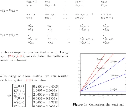
In this example we assume that z = 0. Using Eqs. (2.9)-(2.10), we calculated the coefficients matrix as following:
With using of above matrix, we can rewrite the linear system (2.10) as follows:
W
F(0, r)
F′(0, r)
F′′(0, r)
F(0, r)
F′(0, r)
F′′(0, r)
=
0.2500r−0.4166 1.6667−2.0000r
2.0000r−3.3333 0.0833−0.2500r
2.0000r−2.3333 0.6666−2.0000r
The vector solution of above linear system is:
F(0, r)
F′(0, r)
F′′(0, r)
F(0, r)
F′(0, r)
F′′(0, r)
=
0
r
0 0 2−r
0
Approximate solution and exact solution are compared in Fig. 1 for r= 0,0.5,1.
After propagating this solution in Eq. (2.7), the calculated solution is equal to exact solution. In other words, with using of this method we can find the analytical solution for this kind of equation, if the exact solution of given problem be a polynomial.
Example 4.2 Let fuzzy integral equation
f(t, r) =
3(r2−2)(3t2+2)−t3(3r2−6)−r(r4+2)(9t2−10),
Figure 1: Comparison the exact and ap-proximated solutions for Example4.1.
f(t, r) =
3(r2−2)(9t2−10)+t3(r5+2r)−r(r4+2)(3t2+2),
k(s, t) = 3(2−s2+t2), 0≤s, t≤2,
with the exact solution F(t, r) = t3(6− 3r2),
F(t, r) =t3(r5+ 2) and a= 0,b= 2, λ= 1. By using Eqs. (2.9)-(2.10), we worked as following:
W =
W1,1 W1,2 W2,1 W2,2 ,
W1,1=
4.6569 3.0000 1.1314 0.33333 0.0808 0.0000 −1.0000 0.0000 0.0000 0.0000 8.4853 6.0000 1.8284 1.0000 0.2828 0.0000 0.0000 0.0000 −1.0000 0.0000 0.0000 0.0000 0.0000 0.0000 −1.0000
-0.7500 0.0416 0.0052 -0.2500 -0.2083 -0.0885 -1.0000 -1.1667 -0.0208 1.0000 0.8333 0.3541 W= 2.0000 0.3333 -0.9583 -2.0000 -1.6667 -0.7083
-0.2500 -0.2083 -0.0885 -0.7500 0.0416 0.0052 1.0000 0.8333 0.3541 -1.0000 -1.1667 -0.0208 -2.0000 -1.6667 -0.7083 2.0000 0.3333 -0.9583
W1,2 =
−1.656 −3.000 −2.731 −1.666 −0.766 0.000 0.000 0.000 0.000 0.000 3.514 6.000 5.171 3.000 1.372 0.000 0.000 0.000 0.000 0.000 0.000 0.000 0.000 0.000 0.000
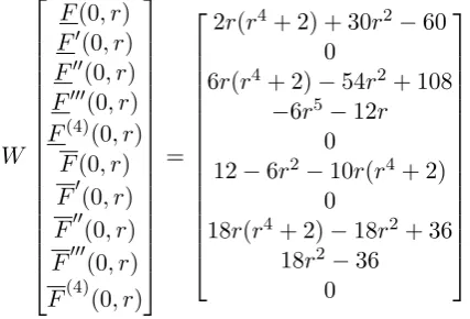
Now we can write system (2.10) as follows:
W
F(0, r)
F′(0, r)
F′′(0, r)
F′′′(0, r)
F(4)(0, r)
F(0, r)
F′(0, r)
F′′(0, r)
F′′′(0, r)
F(4)(0, r)
=
2r(r4+ 2) + 30r2−60 0
6r(r4+ 2)−54r2+ 108 −6r5−12r
0
12−6r2−10r(r4+ 2) 0
18r(r4+ 2)−18r2+ 36 18r2−36
0
The vector solution of the above linear system is:
F(0, r)
F′(0, r)
F′′(0, r)
F′′′(0, r)
F(4)(0, r)
F(0, r)
F′(0, r)
F′′(0, r)
F′′′(0, r)
F(4)(0, r)
= 0 0 0 6r(r4+ 2)
0 0 0 0 −18(r2−2)
0
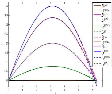
Approximate solution and exact solution are compared in Fig. 2 forr= 0,0.5,1.
As showed, the exact solution and approxi-mate solution are equal.
Figure 2: Comparison the exact and ap-proximated solutions for Example4.2.
Example 4.3 Let fuzzy integral equation
f(t, r) =sin(t 2)((
13 15)(r
2+r) + ( 2
15)(4−r
3−r)),
f(t, r) =sin(t 2)((
2 15)(r
2+r) + (13
15)(4−r
3−r)),
k(s, t) = 0.1sin(s)sin(t
2), 0≤s, t≤2Π,
with the exact solutionF(t, r) = (4−r3−r)sin(2t),
F(t, r) = (r2+r)sin(2t)anda= 0,b= 2π, λ= 1.
Similarly by using Eqs. (2.9)-(2.10), we calcu-lated the coefficients matrix W in z = 0 as fol-lowing:
W =
W1,1 W1,2 W2,1 W2,2 ,
W1,1=
−1.00 0.000 0.000 0.000 0.000 0.000 0.100 −0.84 0.146 0.101 0.056 0.026 0.000 0.000 −1.00 0.000 0.000 0.000 −0.02 −0.03 −0.03 −1.02 −0.01 −0.00 0.000 0.000 0.000 0.000 −1.00 0.000 0.006 0.009 0.009 0.006 0.003 −0.99
W1,2 =
0.000 0.000 0.000 0.000 0.000 0.000 −0.10 −0.47 −1.13 −1.85 −2.31 −2.35 0.000 0.000 0.000 0.000 0.000 0.000 0.025 0.117 0.283 0.463 0.579 0.588 0.000 0.000 0.000 0.000 0.000 0.000 −0.00 −0.02 −0.07 −0.11 −0.14 −0.14
.
Now we van write: (2.10) as follows:
W
F(0, r)
F′(0, r)
F′′(0, r)
F′′′(0, r)
F(4)(0, r)
F(5)(0, r)
F(0, r)
F′(0, r)
F′′(0, r)
F′′′(0, r)
F(4)(0, r)
F(5)(0, r)
= 0 r3 15− 13r2
30 − 11r
300− 4 15
0 −r3
60+ 13r2
120 + 11r 120 + 1 15 0 r3 240 − 13r2
480 − 11r 480 − 1 60 0
13r3
30 − r2 15+ 11r 30 − 26 15 0 −13r3
120 + r2 60− 11r 120 + 13 30 0
13r3
480 − r2 240 + 11r 480 − 13 120
The vector solution of above linear system is:
F(0, r)
F′(0, r)
F′′(0, r)
F′′′(0, r)
F(4)(0, r)
F(5)(0, r)
F(0, r)
F′(0, r)
F′′(0, r)
F′′′(0, r)
F(4)(0, r)
F(5)(0, r)
= 0
0.0127r3+ 0.5023r2+ 0.5151 r−0.0511 0
−0.0031r3−0.1255r2−0.1287r+ 0.0127 0
0.0007r3+ 0.0313r2+ 0.03219 r−0.0031 0
−0.5023r3−0.0127r2−0.5151r+ 2.0093 0
0.1255r3+ 0.0031r2+ 0.1287 r−0.5023 0
−0.0313r3−0.0007r2−0.0321r+ 0.1255
Fig. 3 shows the accuracy of the solution functions. The differences between 6-th trunca-tion limits of Taylor series with exact solutrunca-tion are quite noticeable.
Figure 3: Comparison the exact and ap-proximated solutions for Example4.3.
From this example, we can conclude that to get the best approximating solution for unknown functions, the truncation limit N must be chosen large enough.
5
Conclusion
In some cases an analytical solution can not be found for integral equation, therefore numerical methods have been applied. In this paper we have worked out a computational method for the ap-proximate solution of the linear Fredholm fuzzy integral equations of the second kind. the pre-sented course in this study is a method for com-puting unknown Taylor coefficients of the solution functions. Consider that to get the best approxi-mating solution of the present fuzzy equation, the truncation limit N must be chosen large enough. An interesting feature of this method is finding the analytical solution for given equation, if the exact solution was a polynomial of degree N or less than N. The analyzed examples illustrate the ability and reliability of the present method.
References
and Adomians decomposition method, Appl. Math. Comput. 173 (2006) 493-500.
[2] G. Alefeld, J. Herzberger, Introduction to in-terval computations, Academic Press, New York, 1983.
[3] E. Babolian, H. Sadeghi Goghary, S. Abbas-bandy, Numerical solution of linear Fredholm fuzzy integral equations of the second kind by Adomian method, Appl. Math. Comput. 161 (2005) 733-44.
[4] W. Congxin, M. Ming, On the integrals, se-ries and integral equations of fuzzy set-valued functions, J. Harbin. Inst. Technol. 21 (1990) 9-11.
[5] M. El-Shahed, Application of Hes homo-topy perturbation method to Volterras integro-differential equation, Int. J. Non. Sci. Num. Simul. 6 (2005) 163-168.
[6] M. Friedman, M. Ma, A. Kandel, Numeri-cal solutions of fuzzy differential and integral equations, Fuzzy Sets Syst. 106 (1999) 35-48.
[7] R. Goetschel, W. Voxman,Elementary calcu-lus, Fuzzy Sets Syst. 18 (1986) 31-43.
[8] A. Golbabai, B. Keramati,Modified homotopy perturbation method for solving Fredholm in-tegral equations, Chaos Soli. Frac. 3 (2006) 45-56.
[9] M. Gulsu, M. Sezer, The approximate solu-tion of high order linear difference equasolu-tion with variable coefficients in terms of Taylor polynomials, Appl. Math. Comput. 168 (2005) 76-88.
[10] H. Hochstadt, Integral equations, New York: Wiley; 1973.
[11] O. Kaleva, Fuzzy differential equations, Fuzzy Sets Syst. 24 (1987) 301-317.
[12] R. P. Kanwal , K. C. Liu,A Taylor expansion approach for solving integral equations, Int. J. Math. Educ. Sci. Technol. 20 (1989) 411-414.
[13] X. Lan, Variational iteration method for solving integral equations, Comput. Math. Appl. 54 (2007) 1071-1078.
[14] S. J. Liao, Beyond Perturbation: Introduc-tion to the Homotopy Analysis Method, Chap-man Hall/CRC Press, Boca Raton, 2003.
[15] S. J. Liao,On the homotopy analysis method for nonlinear problems, Appl. Math. Comput. 147 (2004) 499-513.
[16] S. J. Liao, Notes on the homotopy analysis method: some definitions and theorems, Com-munications in Nonlinear Science and Numer-ical Simulation (2008),http://dx.doi.org/ 10.1016/j.cnsns.2008.04-013/.
[17] S. J. Liao, Y. Tan, A general approach to obtain series solutions of nonlinear differen-tial equations, Stud. Appl. math. 119 (2007) 297-355.
[18] K. Maleknejad, N. Aghazadeh, Numerical solution of Volterra integral equations of the second kind with convolution kernel by using Taylor-series expansion method, Appl. Math. Comput. 161 (2005) 915-922.
[19] S. Nas, S. Yalnba, M. Sezer, A Taylor poly-nomial approach for solving high-order linear Fredholm integrodifferential equations, Int. J. Math. Educ. Sci. Technol. 31 (2000) 213-225.
[20] S. Nas, S. Yalnba, M. Sezer, A Taylor poly-nomial approach for solving high-order linear Fredholm integrodifferential equations, Int. J. Math. Educ. Sci. Technol. 31 (2000) 213-225.
[21] H. T. Nguyen,A note on the extension prin-ciple for fuzzy sets, J. Math. Anal. Appl. 64 (1978) 369-380.
[22] M. L. Puri, D. Ralescu, Fuzzy random vari-ables, J. Math. Anal. Appl. 114 (1986) 409-22.
[23] F. G. Tricomi, Integral equations, Dover Publications, New York, 1982.
[24] S. Yalcinbas, Taylor polynomial solutions of nonlinear VolterraFredholm integral equa-tions, Appl. Math. Compt. 127 (2002) 195-206.
[26] L. A. Zadeh, Toward a generalized theory of uncertainty (GTU) an outline, Inform. Sci. 172 (2005) 1-40.
[27] L. A. Zadeh,The concept of a liguistic vari-able and its application to approximate rea-soning: Parts 1-3, Inform. Sci. 8 (1975) 199-249, 301-357; 9 (1975) 43-80.
Ahmad Jafarian was born in 1978 in Tehran, Iran. He received B. Sc (1997) in Applied mathematics and M.Sc. in applied mathemat-ics from Islamic Azad University Lahi-jan Branh to Lahijan, Fer-dowsi University of Mashhad re-spectively. He is a Assistant Prof. in the depart-ment of mathematics at Islamic Azad University, Urmia Branch, roumieh, in Iran. His current in-terest is in artificial intelligence, solving nonlinear problem and fuzzy mathematics.