Computational technique of linear partial differential equations by reduced differential transform ‎method

(1)

Vol. 8, No. 4, 2016 Article ID IJIM-00651, 7 pages Research Article

Computational technique of linear partial differential equations by

reduced differential transform method

H. Rouhparvar ∗†

Received Date: 2015-01-23 Revised Date: 2016-01-01 Accepted Date: 2016-08-14

————————————————————————————————–

Abstract

This paper presents a class of theoretical and iterative method for linear partial differential equations. An algorithm and analytical solution with a initial condition is obtained using the reduced differential transform method. In this technique, the solution is calculated in the form of a series with easily com-putable components. There test modeling problems from mathematical mechanic, physic, electronic and so on, and are discussed to illustrate the effectiveness and the performance of the our method.

Keywords : Reduced differential transform method; Taylor series; Parabolic equations; Hyperbolic equations.

—————————————————————————————————–

1 Introduction

L

inear partial differential equations (LPDEs)arise in the formulation of fundamental laws of nature and in the mathematical analysis of a wide variety of problems in applied mathematics, mathematical physic, mechanic and engineering science. For instance,

1- The heat or diffusion equation: this equation describes the diffusion of thermal energy in a medium. It can be used to model the flow of a quantity, such as heat, or a concentration of particles. It is also used as a model equa-tion for growth and diffusion, in general, and growth of a solid tumor, in particular.

2- The wave equation: this equation describes the propagation of a wave (or disturbance), and it arises in a wide variety of physical

∗_{Corresponding author. [email protected]} †_{Department of Mathematics, College of Technical}

and Engineering, Saveh Branch, Islamic Azad University, Saveh, Iran.

problems. Some of these problems include a vibrating string, longitudinal vibrations of an elastic rod or beam, transmission of elec-tric signals along a cable.

3- The telegraph equation: this equation arises in the study of propagation of electrical sig-nals in a cable of a transmission line.

4- And so on [15].

Many problems of physical are described by LPDEs with appropriate initial and/or boundary conditions. In this paper, the reduced differential transformation method (RDTM) is presented for LPDEs with initial conditions in a general form. Also, a recursive formula of the RDTM is introduced that is applied for a wide variety of LPDEs specially of the types parabolic and hyperbolic equations.

(2)

2 Differential

transform

method (DTM)

The DTM was first proposed by Zhou [16], who solved linear and nonlinear initial value problems in electric circuit analysis, and was used heav-ily in the literature successfully applied to eigen-value problems [7], one-dimensional planar Bratu problem [1], higher-order initial value problems [2,8], systems of ordinary and partial differential equations [3, 5], high index differential-algebraic equations [14], integro-differential equations [4].

2.1 Two dimensional the differential transform method

The basic definitions and fundamental operations of the two-dimensional differential transform are introduced in [9] as the following

W(k, h) = 1 k!h!

[

∂k+h

∂xk_∂thw(x, t) ]

(0,0)

, (2.1)

wherew(x, t) is the original function andW(k, h) is the transformed function. The differential in-verse transform of W(k, h) is

w(x, t) = ∞

∑

k=0 ∞

∑

h=0

W(k, h)xkth, (2.2)

and from Eqs. (2.1) and (2.2) can be concluded

w(x, t) =

∑_∞ k=0

∑_∞ h=0

1

k!h!

[ ∂k+h

∂xk_∂thw(x, t) ]

(0,0)x

k_th_.

(2.3) In Table 1 has listed the fundamental mathe-matical operations of two-dimensional differential transform. The proofs of Table1 are available in [6].

2.2 The reduced differential transform method

The basic definitions and operations of the RDTM [11,12,13] are defined as follows:

Definition 2.1 If function u(x, t) is analytic and differentiated continuously with respect to

timetand spacexin the domain of interest, then

let

Uk(x) =

1 k!

[

∂k ∂tku(x, t)

]

t=0

, (2.4)

where the t-dimensional spectrum functionUk(x)

is the transformed function. In this paper, the

lowercase u(x, t) represent the original function

while the uppercase Uk(x) stand for the

trans-formed function.

Definition 2.2 The reduced differential

trans-form of a sequence {Uk(x)}∞k=0 is introduced as

follows:

u(x, t) = ∞

∑

k=0

Uk(x)tk. (2.5)

To combining equation (2.4) and (2.5), we have

u(x, t) = ∞

∑

k=0 1 k!

[

∂k ∂tku(x, t)

]

t=0

tk. (2.6)

Some basic properties of the reduced differential transformation obtained from definitions (2.4) and (2.6) are summarized in Table2. The proofs of Table2and the basic definitions of the RDTM are available in [10].

3 The RDTM for LPDE

Our main result is an application of the RDTM for LPDE. Consider the following LPDE

∑N−1

n=0 an(x, t)Gnu(x, t) +GNu(x, t) =

∑M

m=1bm(x, t)Hmu(x, t) +f(x, t),

(3.7)

with the initial conditions

Gnu(x,0) =gn(x), 0≤n≤N −1, (3.8)

where

Gn= ∂ n

∂tn, 0≤n≤N,

Hm= ∂ m

∂xm, 1≤m≤M.

The approximate solution using the t partial so-lution is given by

u(x, t) =ψ+G−_N1(f(x, t)) +

G−_N1(∑M_m₌₁bm(x, t)Hmu(x, t) )

−G−_N1(∑N_n₌₀−1an(x, t)Gnu(x, t) )

, (3.9) where

ψ=u(x,0) +tut(x,0) +· · ·

+tN−1∂N_∂t−1Nu−(x,10) =g0(x) +tg1(x) +· · ·

+₍_N₋1_1)!tN−1gN−1(x) =

∑N−1

(3)

Table 1: Two dimensional differential transformation

Orig. Fun. Transformed Fun.

u(x, t)±v(x, t) U(k, h)±V(k, h)

cu(x, t) cU(k, h)

∂u(x,t)

∂x (k+ 1)U(k+ 1, h)

∂u(x,t)

∂t (h+ 1)U(k, h+ 1)

∂r+su(x,t)

∂xr_∂ts

(k+r)!

k!

(h+s)!

h!

U(k+r, h+s)

u(x, t)v(x, t)

∑k r=0

∑h s=0

U(r, h−s)V(k−r, s)

Table 2: Basic operations of RDTM

Orig. Fun. Transformed Fun.

u(x, t) Uk(x)

u(x, t)±v(x, t) Uk(x)±Vk(x)

cu(x, t) cUk(x) c is a cons.

xmtn xmδ(k−n)

xm_tn_u₍_{x, t}₎ _xm_U

k₋n(x) ∂

∂xu(x, t)

∂ ∂xUk(x) ∂r

∂tru(x, t)

(k+r)!

k! Uk+r(x)

u(x, t)v(x, t) ∑k_r₌₀Ur(x)Vk−r(x)

and

G−_N1=

∫ t

0

∫ t

0

· · ·

∫ t

0

(.)dtdt_{| {z }}· · ·dt

N times

. (3.10)

According to the RDTM, we consider the transformations of the functions u(x, t), f(x, t), an(x, t) and bm(x, t) as the following

u(x, t) =∑∞_k₌₀Uk(x)tk,

f(x, t) =∑∞_k₌₀Fk(x)tk,

an(x, t) = ∑_∞

k=0An,k(x)tk,

bm(x, t) =∑∞_k₌₀Bm,k(x)tk,

where

Uk(x) = _k1_! [

∂k ∂tku(x, t)

]

t=0,

Fk(x) = _k1_! [

∂k ∂tkf(x, t)

]

t=0,

An,k(x) = _k1_! [

∂k

∂tkan(x, t) ]

t=0,

Bm,k(x) = _k1_! [

∂k

∂tkbm(x, t) ]

t=0,

(3.11)

and 0≤n ≤N −1, 1 ≤m ≤M. To substitute the relations (3.11) into Eq. (3.9), we have

∑_∞

k=0Uk(x)tk= ∑N−1

l=0 l1!t

l_g l(x)+

G−_N1(∑∞_k₌₀Fk(x)tk )

+G−_N1(∑M_m₌₁∑∞_k₌₀Ωm,k(x)tk )

−G−_N1(∑N_n₌₀−1∑∞_k₌₀Φn,k(x)tk )

,

(3.12)

where by Table 2, Ωm,k(x) and Φn,k(x) are as

follows

Ωm,k(x) = ∑k

r=0Bm,r(x)HmUk−r(x),

Φn,k(x) = ∑k

r=0

(k−r+n)!

(4)

We now perform the integrations (3.10) on the Eq. (3.12) to write

∑_∞

k=0Uk(x)tk = ∑N−1

l=0

tl

l!gl(x) +

∑_∞ k=0

k!tk+N

(k+N)!Fk(x)

+∑∞_k₌₀∑k_r₌₀∑M_m₌₁k₍_k!₊tk_N+N_)!

Bm,r(x)HmUk−r(x)

−∑∞k=0

∑k r=0

∑N−1

n=0

(k−r+n)!k!tk+N

(k−r)!(k+N)!

An,r(x)Uk−r+n(x).

(3.13) Letk→k−N on the right side, then

∑_∞

k=0Uk(x)tk= ∑N−1

l=0

tl

l!gl(x) +

∑_∞ k=N

(k−N)!tk

k! Fk−N(x)

+∑∞_k₌_N∑k_r₌₀−N∑M_m₌₁ (k−N_k_!)!tk

Bm,r(x)HmUk−N−r(x)

−∑∞k=N ∑k−N

r=0

∑N−1

n=0

(k−N−r+n)! (k−N)!tk

(k−r)!k!

An,r(x)Uk−N−r+n(x).

(3.14) At last, equation coefficients of the same powers of t, we obtain the recursive formula for coeffi-cients as the following

U0(x) =g0(x), U1(x) =g1(x), . . . ,

UN−1(x) = ₍_N₋1_1)!gN−1(x),

(3.15)

and

Uk+N(x) = ₍_k₊k_N! _)!Fk(x)+ ∑k

r=0

∑M m=1

k!

(k+N)!Bm,r(x)HmUk−r(x)

−∑k r=0

∑N−1

n=0

(k−r+n)!k! (k−r)!(k+N)!

An,r(x)Uk−r+n(x),

k= 0,1,2, . . . .

(3.16)

Substituting (3.15) into (3.16) and by a straight forward iterative calculations, we obtain the fol-lowing Uk(x) values. So, the inverse

transforma-tion of the set of values {Uk(x)}p_k₌₀ give

approx-imate solution as

up(x, t)≈ p ∑

k=0

Uk(x)tk,

where p is order of approximation solution. In result,the exact solution of problem is given by

u(x, t) = lim

p→∞up(x, t).

Let us consider the error functional forp-order approximate solution as the following

Error(x, t) =

|∑N−1

n=0 an(x, t)Gnup(x, t) +GNup(x, t)

−∑M

m=1bm(x, t)Hmup(x, t)−f(x, t)|.

(3.17)

4 Applications

The recursive formula (3.16) with (3.15) applies for a rather wide class of the LPDEs to the ini-tial conditions. As application, we consider the examples of parabolic and hyperbolic equations.

4.1 The parabolic equations

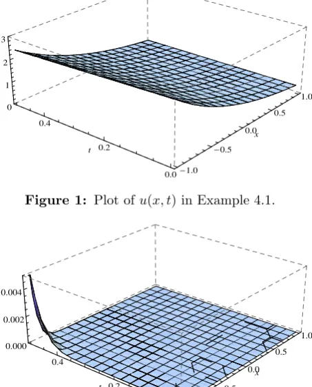
Example 4.1 A parabolic equation that de-scribes heat transfer in a quiescent medium (solid body) in the case where thermal diffusivity is an exponential function of the coordinate as the fol-lowing

∂u ∂t =a(e

βx∂2u

∂x2 +βe

βx∂u

∂x), (4.18) whereaandβare constant. By attention to (3.7), we have

N = 1, M = 2, a0(x, t) = 0, f(x, t) = 0,

b1(x, t) =aβeβx, b2(x, t) =aeβx,

and assume that the initial condition is u(x,0) = e−x. Therefore, from (3.16) we obtain

U0(x) =e−x,

Uk+1(x) =

∑k

r=0 k+11 (B1,r(x)

∂

∂xUk−r(x)

+B2,r(x)∂ 2

∂x2Uk−r(x))

−∑k r=0

1

k+1A0,r(x)Uk−r(x),

k= 0,1,2, . . . ,

(4.19) where B1,r(x), B2,r(x) and A0,r(x) are

deter-mined by (3.11). We consider

a= 0.05, β =−1, p= 15,

(5)

-1.0 -0.5

0.0 0.5

1.0

x

0.0 0.2

0.4

t

0 1 2 3

Figure 1: Plot ofu(x, t) in Example 4.1.

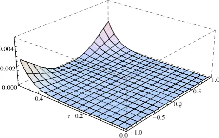
-1.0 -0.5

0.0 0.5

1.0

x

0.0 0.2

0.4

t

0.000 0.002 0.004

Figure 2: Plot ofError(x, t) in Example 4.1.

Example 4.2 Another parabolic equation is con-taining trigonometric function and arbitrary pa-rameters as the following

∂u ∂t =a

∂2u ∂x2 +b

∂u

∂x+ (ccos

h_ωt₊_s₎_u, _(4.20)

wherea, b, c, h, sand ω are constant. From (3.7), we have

N = 1, M = 2, a0(x, t) =ccoshωt+s,

b1(x, t) =b, b2(x, t) =a, f(x, t) = 0,

and suppose that the initial condition isu(x,0) = sint. Hence, by (3.16) we obtain

U0(x) = sint,

Uk+1(x) =

∑k

r=0 k+11 (B1,r(x)

∂

∂xUk−r(x)

+B2,r(x)∂ 2

∂x2Uk−r(x))

−∑k

r=0k+11 A0,r(x)Uk−r(x),

k= 0,1,2, . . . ,

(4.21) where B1,r(x), B2,r(x) and A0,r(x) are

deter-mined by (3.11). Let us consider

a= 0.5, b= 0.5, c= 0.1, s=−0.5,

h= 2, ω=π, p= 10.

By attention to (4.21), the approximate solution and error functional have been shown in figures (3) and (4), respectively.

-1.0 -0.5

0.0 0.5

1.0

x

0.0 0.2

0.4

t

-1.0 -0.5

0.0 0.5 1.0

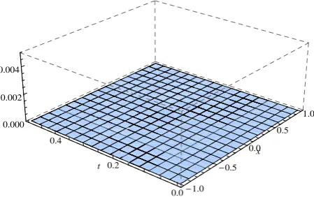
-1.0 -0.5

0.0 0.5

1.0

x

0.0 0.2

0.4

t

0.000 0.002 0.004

4.2 The hyperbolic equations

Example 4.3 Let consider the hyperbolic equa-tion

∂2u ∂t2 =α

2∂2u ∂x2 −β

∂u

∂t, (4.22) where α and β are constant. This equation gov-erns free transverse vibration of a string, and also longitudinal vibration of a rod in a resisting medium with a velocity-proportional resistance coefficient. By attention to (3.7), we have

N = 2, M = 2, a0(x, t) = 0, a1(x, t) =β,

b1(x, t) = 0, b2(x, t) =α2, f(x, t) = 0,

and also assume that the initial conditions are

u(x,0) = sinx2,

ut(x,0) =ex 2

(6)

So, from (3.16) we obtain

U0(x) = sinx2,

U1(x) =ex2,

Uk+2(x) =

∑k

r=0 (k+1)(1k+2)B2,r(x)

∂2

∂x2Uk−r(x)

−∑k r=0

k−r+1

(k+1)(k+2)A1,r(x)

∂

∂tUk−r+1(x),

k= 0,1,2, . . . ,

(4.23) where B2,r(x) and A1,r(x) are determined by

(3.11). We consider

α= 1, β = 1, p= 10,

and obtain the approximate solution by (4.23). The approximate solution and error functional have been shown in figures (5) and (6), respec-tively.

-1.0 -0.5

0.0 0.5

1.0

x

0.0 0.2

0.4

t

0 1 2 3

-1.0 -0.5

0.0 0.5

1.0

x

0.0 0.2

0.4

t

0.000 0.002 0.004

Example 4.4 We consider the second hyperbolic equation as the following

∂2u ∂t2 +c

∂u ∂t =a

2∂2u

∂x2 −bu+f(x, t), (4.24)

wherec, aandbare constant. Ifc >0, b <0 and f(x, t) = 0, then this equation is called the tele-graph equation whereucan be voltage or current through the wire. From (3.7), we have

N = 2, M = 2, a0(x, t) =b, a1(x, t) =c,

b1(x, t) = 0, b2(x, t) =a2, f(x, t) =ext2,

and consider the initial conditions as follows

u(x,0) = cosx2,

ut(x,0) =xsinx2.

Therefore, from (3.16) we obtain

U0(x) = cosx2,

U1(x) =xsinx2,

Uk+2(x) = ₍_k₊₁₎₍1_k₊₂₎Fk(x)

+∑k_r₌₀₍_k₊₁₎₍1_k₊₂₎B2,r(x) ∂ 2

∂x2Uk−r(x)

−∑k

r=0(k+1)(1k+2)A0,r(x)Uk−r(x)

−∑k

r=0(k+1)(k−r+1k+2)A1,r(x)

∂

∂tUk−r+1(x),

k= 0,1,2, . . . ,

(4.25) whereFk(x),B2,r(x),A0,r(x) andA1,r(x) are

de-termined by (3.11). We consider

a= 0.5, b=−1, c= 0.8, p= 10,

and obtain the approximate solution by (4.25). The approximate solution and error functional have been shown in figures (7) and (8), respec-tively.

-1.0 -0.5

0.0 0.5

1.0

x

0.0 0.2

0.4

t

0.0 0.5 1.0 1.5 2.0

5 Conclusion

(7)

-1.0 -0.5

0.0 0.5

1.0

x

0.0 0.2

0.4

t

0.000 0.002 0.004

form and obtained a recursive formula, i.e. (3.16) with (3.15), that can be used in another science and engineering by a software code of the Mathe-matica or Matlab software. The recursive formula is a rapidly method because it uses of differenti-ation that this operator consume the little time of computer at computations. Also, by attention to examples, is saw where the method has much carefulness.

Acknowledgements

The author would like to appreciate the anony-mous reviewers for their helpful comments.

References

[1] I. H. Abdel-Halim Hassan, Vedat Suat Ertrk,

Applying differential transformation method to the one-dimensional planar Bratu prob-lem, Int. J. Contemp. Math. Sciences 2 (2007) 1493-1504.

[2] I. H. Abdel-Halim Hassan, Differential transformation technique for solving

higher-order initial value problems, Appl. Math.

Comput. 154 (2004) 299-311.

[3] I. H. Abdel-Halim Hassan, Application to differential transformation method for

solv-ing systems of differential equations, Appl.

Math. Modell. 32 (2008) 2552-2559.

[4] A. Arikoglu, I. Ozkol, Solution of boundary value problems for integro-differential

equa-tions by using differential transform method,

Appl. Math. Comput. 168 (2005) 1145-1158.

[5] F. Ayaz, Solutions of the systems of dif-ferential equations by difdif-ferential transform

method, Appl. Math. Comput. 147 (2004)

547-567.

[6] F. Ayaz,On the two-dimensional differential

transform method, Appl. Math. Comput. 143

(2003) 361-374.

[7] C. K. Chen, S. H. Ho, Application of dif-ferential transformation to eigenvalue prob-lems, Appl. Math. Comput. 79 (1996) 173-188.

[8] M. J. Jang, C. L. Chen, Y. C. Liy,On solving the initial value problems using the

differ-ential transformation method, Appl. Math.

Comput. 115 (2000) 145-160.

[9] F. Kangalgil, F. Ayaz, Solitary wave solu-tions for the KdV and mKdV equasolu-tions by

differential transform method, Chaos

Soli-tons & Fractals 41 (2009) 464-472.

[10] Y. Keskin, Ph.D. Thesis, Selcuk University, 2010 (in Turkish).

[11] Y. Keskin, G. Oturanc, Reduced tial Transform Method for Partial

Differen-tial Equations, International Journal of

Non-linear Sciences and Numerical Simulation 10 (2009) 741-749.

[12] Y. Keskin, G. Oturanc, Reduced differential transform method for solving linear and

non-linear wave equations, Iranian Journal of

Sci-ence & Technology, Transaction A 34 (2010) 113-122.

[13] Y. Keskin, G. Oturanc, Reduced Differen-tial Transform Method for fractional parDifferen-tial

differential equations, Nonlinear Science

Let-ters A 1 (2010) 61-72.

[14] H. Liu, Yongzhong Song, Differential trans-form method applied to high index

differen-tial algebraic equations, Appl. Math.

Com-put. 184 (2007) 748-753.

[15] A. D. Polyanin, Handbook of Linear Par-tial DifferenPar-tial Equations for Engineers and

Scientists, Chapman & Hall/CRC (2002).

[16] J. K. Zhou, Differential transformation

(8)

Huarjung University PressWuuhahn, China (1986), (in Chinese).