R E S E A R C H
Open Access
Simulation of blow-up solutions to the
generalized KdV equations by moving
collocation methods
Zhiqiang Zhou
*and Xiaodan Wu
*Correspondence:
[email protected] School of Economic Mathematics, Southwestern University of Finance and Economics, Chengdu, Wenjiang 611130, P.R. China
Abstract
The aim of this paper is to simulate the blow-up solutions to generalized
Korteweg-de Vries (KdV) equations. The KdV equations are discretized with the use of a quintic Hermite collocation method based on the moving meshes generated by solving moving mesh partial differential equations (MMPDEs). Theoretical analyses are, respectively, conducted to determine the critical parameters in MMPDEs such that the generated meshes can catch up with the blow-up profiles and to show the effectiveness of the generated moving meshes. Lastly, a variety of examples are implemented to confirm our analysis and show the efficiency of the method.
MSC: 35Q51; 35Q53; 65N50; 65N35
Keywords: Korteweg-de Vries equations; moving mesh methods; dimensional analysis; blow-up solution
1 Introduction
The focus of this paper is on numerical simulations of blow-up solutions to the generalized Korteweg-de Vries (GKdV) equation
ut+upux+uxxx= , x∈(a,b), ()
with periodic boundary conditions, whereis a positive number andpa positive integer. The special casep= is the standard KdV equation (e.g., []), andp= corresponds to the modified KdV equation (e.g., []). The theoretical analysis by Bonaet al.[] shows that the solitary-wave solutions are stable if and only ifp< . Bonaet al.[] also show that the solutions forp≥ exhibit finite blow-up phenomena with a similarity form
u(x,t) = (T–t)–/(p)ψ
x∗–x–c(T–t)/
(T–t)/
+ bounded term, ()
wherex∗,T,care real parameters and the similarity profileψis a smooth function which tends to zero at±∞. The point at which the peak value occurs depends on time in the formx(t) =x∗+c(T–t)/, and, obviously,x→x∗ast→T.
To compute such a type of singularities sufficiently and effectively, and hence to mimic the asymptotic behavior of the solution ast→T, the numerical method employed is re-quired to adapt the spatial meshes to the evolving singularities. In order to achieve this, Bonaet al.employ theh-adaptation technique [, ]: a spatial translation is used to keep the blow-up peak appearing near the fixed pointx= . and local mesh refinement is con-ducted recursively right around this point. The demerit of this local refinement technique is that the computational cost becomes larger and larger as the blow-up solution evolves. Moreover, the use of interpolations in the time integration does not keep the truncation errors under control. In this paper, based on the moving mesh method, we provide a more reliable simulation method along with an in-depth analysis.
Let a coordinate be
μ=x–x∗–c(T–t)/(T–t)–/. ()
Then the blow-up profile can be represented by this coordinate. The mesh movement is based on the time-dependent mapping
x(·,t) :Ic→I= [xL,xR],
wherexL,xRare the left and right boundary points for the physical equation, andIcis a
computational space in which uniform grids will be taken. WhenIcis taken as [, ] for
example, the moving mesh can be generated byxj(j/N,t),j= , , . . . ,N. The functionu(x,t)
in physical variables can be transformed into the function in computational variables
u(x,t) =ux(ξ,t),t,
and the blow-up profile is expressed in the computational variableξ. Equation () suggests that in order to keep up with the blow-up profiles, the mesh trajectory speed has to satisfy
[x˙] =[x] [t] ≥[t]
–/, ()
whereafter we use [u], [t], and [x] to denote the dimensions of the variablesu,t, andx, re-spectively. For the underlying physical PDEs () the time scale should be taken as [t] =T–t. Dimensional analysis, more often used by physicians, is a tool to find or check relations among physical quantities. In our paper, we use this technique to approximately determine the relations among some dominant quantities in the equation with blow-up solutions, and this method was first used by Buddet al.in [].
The moving mesh functionx(ξ,t) satisfies certain parabolic equations which are called moving mesh partial differential equations (MMPDEs). Two MMPDEs (MMPDE, MM-PDE) in [] are considered in this paper, namely,
˙
x= τ
∂ ∂ξ
M∂x ∂ξ
, ()
–∂
x˙
∂ξ=
τ
∂ ∂ξ
M∂x ∂ξ
with
x(,t) =a, x(,t) =b. ()
HereM=M(x,t) is the monitor function which depends on the physical solution and is used for controlling mesh concentration, whileτ=τ(t) > is a parameter used for adjust-ing the response time of mesh movement to changes inM. The two MMPDEs are obtained based on attraction and repulsion pseudoforces between nodes. They are also related to the equidistribution equation,
= ∂ ∂ξ
M∂x ∂ξ
. ()
It can be observed that, for both MMPDE and MMPDE, the mesh trajectory speeds depend onMandτ. Moreover, for any choice ofMandτ, the two MMPDEs can generate smooth meshes as long as the time scale is taken to be sufficiently small. Therefore, the key issues we need to deal with in the simulation of blow-up are: . how to chooseMandτ so that the mesh trajectory speed is as fast as that in (); . how small the time scale should be in order that the MMPDEs can generate smooth meshes and resolve the dramatically increase in the blow-up solution.
The dimensional equation for both MMPDE and MMPDE is
[x˙] =[M][x] [τ] .
In view of (), to capture the blow-up profiles, it is required that
[M][x] [τ] ≥[t]
–/. ()
2 The conservative moving collocation method
The conservative moving collocation method, which is introduced by Huang and Russell [], will be used to discretize the main equation. To this end, we reformulate the GKdV equation () into the following form:
F(ut) =
G(u,uxx)
x, ()
whereF(ut) =utandG(u,uxx) = –p+ up+–uxx. Define a time mesh
=t<t<· · ·<tL.
Denote the time-dependent spatial mesh at timetn(n= , , . . .) by
a=xn<xn <· · ·<xnN =b.
Denote the size of thejth interval byhn
j =xnj –xnj–, j= , , . . . ,N. Divide each interval
equally into three parts by inserting two pointsxn j+k =x
n j +kh
n
j+,k= , . Integrating ()
overInj,k= [xn
j+k,x
n
j+k+ ],k= , , , gives
In j,k
F(ut)dx=G(u,uxx)|x=xn j+k+
–G(u,uxx)|x=xn j+k
. ()
On intervals [xn
j,xnj+] (j= , , . . . ,N– ),u(x,tn) is approximated by a fifth-order Hermite
polynomial
vn(x) =vnjφ(s) +vnx,jhnj+φ(s) +vnxx,j
hnj+φ(s)
+vnj+φ(s) +vnx,j+hnj+φ(s) +vnxx,j+
hnj+φ(s),
wherevn
j,vnx,j,vxxn,jdenote the approximations tou(xnj,tn),ux(xnj,tn),uxx(xnj,tn), respectively.
The local coordinatesis defined by
s=x–x
n j
hnj+ ,
and the Hermite basis functions are given by
φ(s) =
–s– s– (s– ), φ(s) = –s(s+ )(s– ), φ(s) = –/s(s– ),
φ(s) =
s– s+ s, φ(s) = –(s– )(s– )s, φ(s) = /(s– )s.
In order to obtain an algorithm which is second order in time, we consider the approxi-mation tou(x,tn–/), wheretn–/≡tn–+tn, defined by
vn–/(x) =v˜
n–
j +vnj
φ(s) +
˜
vnx,–j +vnx,j
h
n j+φ(s) +
˜
vnxx–,j+vnxx,j
hnj+φ(s)
+v˜
n–
j+ +vnj+
φ(s) +
˜
vn–
x,j++vnx,j+
h
n j+φ(s) +
˜
vn–
xx,j++vnxx,j+
forx∈[xnj,xnj+],j= , , . . . ,N– ,u(x,tn–/), where
˜
vnj–=vn–xjn, v˜nx,–j =vxn–xnj, v˜nxx–,j=vnxx–xnj.
Similarly, we define the approximations toux(x,tn–/) anduxx(x,tn–/), respectively, by
vnx–/(x) = hn j+
˜
vn–
j +vnj
φ(s) +
˜
vn–
x,j +vnx,j
h
n j+φ(s) +
˜
vn–
xx,j+vnxx,j
hnj+φ(s)
+v˜
n–
j+ +vnj+
φ(s) +
˜
vn–
x,j++vnx,j+
h
n j+φ(s) +
˜
vn–
xx,j++vnxx,j+
hnj+φ(s)
and
vnxx–/(x) = (hn
j+)
˜
vn–
j +vnj
φ(s) +
˜
vn–
x,j +vnx,j
h
n j+φ(s) +
˜
vn–
xx,j+vnxx,j
hnj+φ(s)
+v˜
n–
j+ +vnj+
φ(s) +
˜
vnx–,j++vnx,j+
h
n j+φ(s) +
˜
vnxx–,j++vnxx,j+
hnj+φ(s)
.
Lastly, we define the approximation tout(x,tn–/) as
vnt–/(x) =v
n j –v˜nj–
tn
φ(s) +
vn x,j–v˜nx–,j
tn
hnj+φ(s) +
vn xx,j–v˜nxx–,j
tn
hnj+φ(s)
+v
n j –v˜nj–
tn
φ(s) +
vn x,j–v˜nx,–j
tn
hnj+φ(s) +
vn
xx,j+–v˜nxx–,j+
tn
hnj+φ(s),
wheretn=tn–tn–.
Substituting the above defined approximations into () gives, fork= , , ;j= , . . . , N– ,
Ijn,k
Fvnt–/(x)dx=Gvn–/,vnxx–/x=xn j+k+
–Gvn–/,vnxx–/x=xn j+k
, ()
subject to periodic boundary conditions
vn=vnN, vnx,=vxn,N, vnxx,=vnxx,N. ()
{(), ()} is the discretization of the original problem (). The integral on the left-hand side of () is computed by the two-point Gauss quadrature formula.
3 Choice of monitor functions
We will consider three types of monitor functions in the MMPDEs for generating the moving mesh, namely
M=|u|γ, ()
M=∂u ∂x
M=α|u|γ+ ( –α)∂u ∂x
γ with <α< . ()
Our numerical results show that the first type (polynomial type) of monitor function is capable of simulating the blow-up phenomena, but it fails to capture the solitary waves. Therefore, the second monitor function based on gradient will be used on the purpose of capturing the blow-up and solitary waves later on. The third monitor function is the average of the first two, in which the parameter <α< is used to control the percentage of the mesh points being distributed to the solitary wave region and the blow-up region. In the following, we determine the parametersγ,γ, andτ using dimensional analysis
introduced in [] such that mesh trajectory speeds satisfy ().
We begin with the physical equation (). The dimensions of the termsut,upux, anduxxx
are
[ut] =
[u] [t],
upux
=[u]
p+
[x] , [uxxx] = [u] [x].
The dimensional balance for the physical PDE implies
[u] [t] =
[u]p+
[x] = [u] [x].
This yields the dimension relations
[x] = [t]/, [u] = [t]–/(p). ()
So if the dimension oftis changed by a factor ofλ> , the dimensions ofxandumust vary by factors ofλ/andλ–/(p), respectively, to keep the physical equation dimensionally
balanced. This suggests a scaling transform
t→λt, x→λ/x, u→λ–/(p)u, () which can easily be proved to make the physical equation invariant. In fact, Bonaet al.[] used the same scaling transformation to obtain the similarity form of the blow-up solution ().
Monitor function M=|u|γ: The dimension analysis for MMPDE or MMPDE gives
[x˙] =[x] [t] =
[u]γ[x] [τ] =
[τ][t]γ/(p)–/. () In the following, we discuss the case with a constantτand that with a varyingτseparately. Constantτ: For the situation of constantτ,i.e.,τ is dimensionless, to make the mesh trajectory speed reach
[x˙]≥[t]–/, ()
it requires
γ
p – ≥
or γ≥ p
For the critical case with
γ=
p
, ()
the constantτ should be sufficiently small to ensure a fast enough mesh trajectory speed. It should also be noted that the smaller the value ofτis taken, the faster is the mesh speed. Therefore, our goal is to choose a suitable value ofτsuch that the mesh moves fast enough to keep up with the moving blow-up profile while not too fast in order to guarantee the generation of smooth meshes.
Moreover, notice that blow-up only occurs in the solution to GKdV equations withp> . Even if we can obtain a satisfactory mesh trajectory speed by choosing a monitor func-tion as|u|γwithγ
≥p, such a large power of the solution will generally result in
over-concentration of the mesh points within the blow-up region and cause the simulation to break down. The same problem also occurs when the monitor function is chosen to be () or (). In view of this, we shall only consider the case thatγ andγ have small values.
In particular, we fixγ=γ= while we vary the value ofτ to obtain a satisfactory mesh
speed in the rest of the paper.
Varyingτ: That () holds requires the dimension relation
[τ]≤[t]–γ/(p)= [u]γ–p/.
This suggests us to chooseτ as
τ(t) =κ
max
x u(x,t)
γ–p/–ε
, ()
whereεis some positive constant, andκ > is a dimensionless constant which should be taken sufficient small for (). With this choice ofτ, the mesh trajectory speed will be fast enough so that the moving meshes generated by MMPDE or MMPDE can timely capture the blow-up profiles.
Monitor function M=|∂∂ux|γ:
For this monitor function, the dimensional equation for both MMPDE and MMPDE is
[x˙] = [u] γ
[τ][x]γ–=
[τ][t]γ/(p)+γ/–/. () For () to be satisfied, we require
[τ]≤[t]–γ/(p)–γ/= [u](+p/)γ–p/.
This suggests us to chooseτ as
τ(t) =κ
max
x u(x,t)
(+p/)γ–p/–ε
, ()
Monitor function M=α|u|γ+ ( –α)|∂u ∂x|
γ with <α< : it is not hard to derive that,
for () to be satisfied,τ should be chosen as
τ=κmin
max
x u(x,t)
γ–p/–ε ,
max
x u(x,t)
(+p/)γ–p/–ε
()
withεandκpositive constants as above.
In the last of this section, we shall consider the choice of time-step sizes in the simulation of blow-up solutions. We take the time steps of the form
tn=
ν [maxxu(x,tn–)]γ
, ()
whereνis a small positive constant. From () we know thatmaxxu(x,tn) is proportional
to (T–tn)–/(p),i.e.,
max
x u(x,tn)∼(T–tn)
–/(p).
Now we estimate that
max
x u(x,tn) –maxx u(x,tn–)
∼(T–tn––tn)–/(p)– (T–tn–)–/(p)
= (T–tn–)–/(p)
– (T–tn)γ/(p)–ν –/(p)
–
≈(T–tn–)–/(p)
p(T–tn)
γ/(p)–ν
=
p(T–tn)
γ/(p)–/(p)–ν. ()
To resolve the dramatic increase in the blow-up solution, we choose
γ = + p/( +ε), ()
whereεis a small positive parameter. The increase in the blow-up solution is then
max
x u(x,tn) –maxx u(x,tn–) =O
(T–tn)εν
.
4 An analysis
In this section, we carry out a careful analysis to verify the validity of MMPDE in sim-ulating blow-up solutions when the monitor functionM,τ are chosen as in {(), ()}, respectively. Similar analysis can be performed for MMPDE with the choice ofM,τ as in {(), ()} or as in {(), ()}. The analysis can also be conducted for MMPDE with the choices ofM,τabove mentioned.
Now we consider () in the blow-up region, that is, timetis close to the blow-up timeT. Write
wherez(ξ) is a smooth function. For simplification, by differentiating (), we obtain
˙
x= c (T–t)
–/+
(T–t)
–/z, ()
xξ = (T–t)/zξ, ()
xξ ξ= (T–t)/zξ ξ. ()
The exact form () gives
u= (T–t)–/(p)ψ(z) + bounded term. () Hereafter we only consider the blow-up solutionuwhile omitting the bounded term. Thus we have
∂u
∂x = (T–t)
–(+p)/(p)ψ(z). ()
Inserting the above expressions into the monitor function () leads to
M=α(T–t)–γ/(p)ψ(z)γ+ ( –α)(T–t)–(+p)γ/(p)ψ(z)γ, Mξ=α(T–t)–γ/(p)
d(|ψ(z)|γ)
dz zξ+ ( –α)(T–t)
–(+p)γ/(p)d(|ψ (z)|γ)
dz zξ.
Putting the above results into
τx˙=M∂
x
∂ξ+
∂M ∂ξ
∂x
∂ξ, ()
which is an equivalent form of MMPDE (), gives
τ c (T–t)
–/+
(T–t)
–/z
=α(T–t)–γ/(p)+/ψ(z)γ
+ ( –α)(T–t)–(+p)γ/(p)+/ψ(z)γ zξ ξ
+ α(T–t)–γ/(p)+/d(|ψ(z)|γ)
dz
+ ( –α)(T–t)–(+p)γ/(p)+/d(|ψ (z)|γ)
dz
zξ. ()
Consider the case that
γ>
+p γ.
Letδ= γ/(p) – ( +p)γ/(p). Multiplying equation () with (T–t)γ/(p)–/gives
τ c (T–t)
γ/(p)–+ (T–t)
γ/(p)–z
=α zξ ξψ(z) γ
+zξ
d(|ψ(z)|γ) dz
+ ( –α)(T–t)δ z
ξ ξψ(z) γ
+zξd(|ψ (z)|γ)
dz
Note that in the blow-up region,z,d(|ψdz(z)|γ), d(|ψdz(z)|γ)are bounded. Combining with () and (), it is not hard to see the term in the left-hand side of () is equal toκO((T–t)ε). By omitting the term on the left-hand side and the second term on the right-hand side in (), we obtain an ODE such that the functionzapproximately satisfies
dz dξ = –
|ψ(z)|γ
d(|ψ(z)|γ) dz
dz dξ
. ()
Similarly, in the case that
γ<
+p γ,
the functionzapproximately satisfies
dz
dξ = –
|ψ(z)|γ
d(|ψ(z)|γ) dz
dz dξ
. ()
For the critical case
γ=
+p γ,
the functionzapproximately satisfies
αψ(z)γ+ ( –α)ψ(z)γd
z
dξ
= – αd(|ψ(z)|
γ)
dz + ( –α)
d(|ψ(z)|γ) dz
dz dξ
. ()
Now we determine the boundary conditions for (), (), (). Since the boundary points are kept to be fixed in the mesh movement (), we know from () that
z() =xL–x∗–c(T–t)/
(T–t)–/; ()
z() =xR–x∗–c(T–t)/
(T–t)–/. ()
To solve the boundary value problems {(), (), ()}, we rewrite the ODE () into the form
d(ddzξ)
dz dξ
= –d(|ψ(z)| γ)
|ψ(z)|γ .
Integrating this equation gives
dz
dξ =Cψ(z)
–γ ,
or
dξ dz =C
–ψ(z)γ ,
Using the boundary condition () and (), we obtain the solution to {(), (), ()}
ξ=
z z()|ψ(s)|
γds
z()
z()|ψ(s)|γds
. ()
Analogously, the solutions to {(), (), ()}, and {(), (), ()} are given by, respec-tively,
ξ=
z
z()|ψ(s)|
γds
z()
z()|ψ(s)|γds
()
and
ξ=
z
z()[α|ψ(s)|
γ+ ( –α)|ψ(s)|γ]ds
z()
z()[α|ψ(s)|γ+ ( –α)|ψ(s)|γ]ds
. ()
Equations (), (), and () indicate that the meshes generated by MMPDE in physical space can equidistribute the correspondent monitor functionsMif the uniform grids are taken inξ space. A similar analysis can be done for other choices of parameters in PDE and MMPDE. This shows the feasibility of determining the parameters in MM-PDE and MMPDE by criterion ().
5 Numerical examples
In this section, we demonstrate the efficiency and accuracy of the proposed moving collo-cation method for solving GKdV equations. Example . is chosen to illustrate the rate of convergence while Examples . and . show the capability of our method to accurately capture the two important features of the GKdV equations - solitary waves and blow-up. The moving collocation method is carried out by solving the coupled system consist-ing of an MMPDE and {(), ()}. We here use MMPDE in the coupled system for our numerical experiments and denoteU(x,tn) the approximate solution obtained attn. The
coupled system attnis solved in an alternating way. To be specific, we choose the monitor
function and the temporal smoothing parameter as follows:
M=g(u,x,t), τ=g(u,t).
We shall first solve MMPDE to generate the spatial mesh attnwith
M(x,tn) =g
U(x,tn–),x,t
, τ(tn) =g
U(x,tn–),t
and then solve {(), ()} on this mesh to obtainU(x,tn).
We mention here that the numerical solution of MMPDE is approximated by using central difference method for the spatial derivatives and backward Euler method for the time derivative.
correction terms in the choice of monitor functions. For instance, when simulating the blow-up profiles in Examples . and ., we choose the monitor function as
M= .|u|+ .|ux|+
(x– )+ .–/+(x– )+ .–/+C, () where the constantCis used to ensure that enough mesh points are distributed away from the blow-up region. We takeC= in our test. The third and the fourth terms are added to guarantee that enough mesh points are distributed around the end points while the first two terms capture the moving blow-up profiles. Based on the choice of monitor functions, we takeτ as in ()
τ= κ
(maxxu(x,t))p/+ε–γ,
withγ= ,εbeing taken as . in our test. The time-step size is taken as in ()
tn=
ν (maxxu(x,tn–))γ
withγ =p+ .
5.1 Convergence rates
We calculate the following example to show the convergence rates of the conservative collocation methods based on fixed and moving meshes.
Example . Consider the GKdV equation () on the space interval [, ] and on the time interval [, ] with the following initial condition:
u(x, ) =Asech/pKx–x, ()
where
K=pAp/(p+ )(p+ )/.
Then the GKdV equation () has the exact solution
u(x,t) =Asech/pKx–x–ωt, () where
ω= KAp/(p+ )(p+ ).
In this experiment, the time stepsize is taken to be t= .×–. We shall vary the
number of mesh subintervalsNto test the order of convergence of our moving collocation method. Both cases, with a uniform mesh and with a moving mesh, are tested. The monitor function is taken as
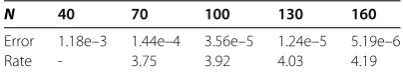
Table 1 Results for the uniform mesh in Example 5.1
N 40 70 100 130 160
Error 1.18e–3 1.44e–4 3.56e–5 1.24e–5 5.19e–6
Rate - 3.75 3.92 4.03 4.19
Table 2 Results for the moving mesh in Example 5.1
N 40 70 100 130 160
Error 1.02e–4 1.34e–5 3.30e–6 1.04e–6 4.06e–7
Rate - 3.63 3.94 4.37 4.57
where applicable. Forp= ,A= ,= ×–,x
= ., the results are shown in Tables
and . In the tables, the rate of convergence is given by
Rate =
log(EN∞ EN∞)
log(/N
/N) .
From Tables and , we may see that the convergence rates for the conservative col-location methods are . The convergence order of the moving colcol-location method with fifth-order Hermite polynomial basis is expected to be ; however, this is only true for some special types of PDE. For the KdV equations which are nonlinear, it is indeed not guaranteed that the moving collocation scheme can attain the sixth-order convergence. The numerical tests show that the conservative collocation methods are of high-order schemes for both fixed (uniform) meshes and moving meshes. Moreover, the error for the moving mesh is smaller than that for fixed (uniform) mesh. In fact, in the literature only one paper by Maet al.[] analyzes the convergence order of moving collocation method for linear second-order PDEs - a very simple PDE; however, it is not possible to prove the convergence rates for nonlinear KdV equations.
5.2 Capture of solitary waves and blow-up
In this section we use two examples to show the capability of our method to accurately capture the two important features of the GKdV equations - solitary waves and blow-up.
Example . Forp= , , we consider the GKdV equation () on the space interval [, ]
with a small perturbation to the initial condition ():
u=λAsech/p
Kx–x, ()
whereλis the perturbation parameter. In our tests, we takeλ= .,A= ,= ×–,
andx= ..
In these tests, the number of mesh subintervals isN= ,κ= .(maxxu(x))
p
Figure 1 Forp= 5 in Example 5.2.The left is the moving meshx(ξ,t) and the right is the blow-up profiles in the computational variableξ.
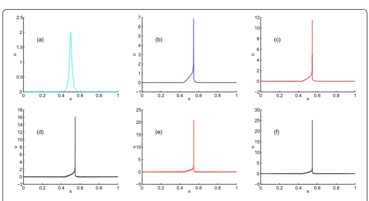
Figure 2 The blow-up profiles forp= 5 in Example 5.2. (a)t= 0,umax= 2.02;
(b)t= 2.249070196709×10⁻²,u
max= 6.249;(c)t= 2.249391515276×10⁻²,umax= 10.58;
(d)t= 2.249397460425×10⁻²,u
max= 14.83;(e)t= 2.249397897417×10⁻²,umax= 19.13;
(f)t= 2.249397956808×10⁻²,u
max= 23.40.
Example . Whenp= , we investigate the GKdV equation () on the space interval
[, ] with the initial profile
u= e–(x–.)
– . ()
In the test we take= .×–. The numerical results are shown in Figures , , in
which the parametersN,κare chosen as in Example . andν= .. The six graphs ofuon the physical space in Figure correspond to the six curves in the right part of Figure .
Figure 3 Forp= 6 in Example 5.2.The left is the moving meshx(ξ,t), the rightu(ξ,t).
Figure 4 The blow-up profiles forp= 6 in Example 5.2. (a)t= 0,umax= 2.02;
(b)t= 5.077843981799×10⁻³,u
max= 6.31;(c)t= 5.077977135290×10⁻³,umax= 10.43;
(d)t= 5.077978558534×10⁻³,u
max= 14.43;(e)t= 5.077978631256×10⁻³,umax= 18.40;
(f)t= 5.077978638853×10⁻³,u
max= 22.33.
6 Conclusions
Figure 5 Forp= 4.The left is moving meshx(ξ,t), the rightu(ξ,t).
Figure 6 The blow-up profiles forp= 4 in Example 5.3. (a)t= 0,umax= 2;(b)t= 7.245823777296×10⁻³, umax= 6.989;(c)t= 7.273839836925×10⁻³,umax= 9.756;(d)t= 7.277618404530×10⁻³,umax= 12.12;
(e)t= 7.278608365592×10⁻³,u
max= 14.22;(f)t= 7.278965443315×10⁻³,umax= 16.12.
Competing interests
The authors declare that they have no competing interests.
Authors’ contributions
XW carried out the analysis in Section 4 and ZZ made the main contributions to the other sections. All authors read and approved the final manuscript.
Acknowledgements
The authors are grateful to Prof. J Ma for the helpful suggestions.
Received: 1 November 2015 Accepted: 26 January 2016 References
1. Korteweg, DJ, de Vries, G: On the change of form of long waves advancing in rectangular canal and on a new type of long stationary wave. Philos. Mag.39, 422-443 (1895)
2. Miura, RM: A remarkable explicit nonlinear transformation. J. Math. Phys.9, 1202-1205 (1968)
3. Bona, JL, Souganidis, PE, Strauss, WA: Stability and instability of solitary waves of KdV type. Proc. R. Soc. Lond. A411, 395-412 (1987)
4. Bona, JL, Weissler, FB: Similarity solutions of the generalized Korteweg-de Vries equation. Math. Proc. Camb. Philos. Soc.127, 323-351 (1999)
5. Bona, JL, Dougalis, VA, Karakashian, OA, McKinney, WR: Conservative, high-order numerical schemes for the generalized Korteweg-de Vries equation. Philos. Trans. R. Soc. Lond. A351, 107-164 (1995)
7. Budd, CJ, Huang, WZ, Russell, RD: Moving mesh methods for problems with blow-up. SIAM J. Sci. Comput.17, 305-327 (1996)
8. Huang, WZ, Ren, Y, Russell, RD: Moving mesh partial differential equations (MMPDEs) based upon the equidistribution principle. SIAM J. Numer. Anal.31, 709-730 (1994)
9. Huang, WZ, Russell, RD: A moving collocation method for the numerical solution of time dependent differential equations. Appl. Numer. Math.20, 101-116 (1996)
10. Russell, RD, Williams, JF, Xu, X: MOVCOL4: a moving mesh code for fourth-order time-dependent partial differential equations. SIAM J. Sci. Comput.29, 197-220 (2007)
11. Ma, J, Jiang, Y: Moving collocation methods for time fractional differential equations and simulation of blowup. Sci. China Math.54, 611-622 (2011)
12. Ma, J, Huang, WZ, Russell, RD: Analysis of a moving collocation method for one-dimensional partial differential equations. Sci. China Math.55, 827-840 (2012)
13. Huang, WZ, Ma, J, Russell, RD: A study of moving mesh PDE methods for numerical simulation of blowup in reaction diffusion equations. J. Comput. Phys.227, 6532-6552 (2008)