A quasi-reversibility regularization method for a Cauchy problem of the modified Helmholtz-type equation

R E S E A R C H

Open Access

A quasi-reversibility regularization method

for a Cauchy problem of the modified

Helmholtz-type equation

Hong Yang

_{and Yanqi Yang}

*_{Correspondence:}

[email protected]

1_{College of Mathematics and}

Statistics, Northwest Normal University, Lanzhou, P.R. China

Abstract

The Cauchy problem of the modified Helmholtz-type equation is severely ill-posed, i.e., the solution does not depend continuously on the given Cauchy data. Thus the regularization methods are required to recover the numerical stability. In this paper, we propose a quasi-reversibility regularization method to deal with this ill-posed problem. Convergence estimates are obtained under a-priori bound assumptions for the exact solution and the selection of regularization parameter. Some numerical results are given to show that this method is stable and feasible.

Keywords: Modified Helmholtz-type equation; Cauchy problem; Quasi-reversibility regularization method; Convergence estimates

1 Introduction

In this study, a Cauchy problem of the Helmholtz-type equation is considered as follows:

⎧ ⎪ ⎪ ⎪ ⎪ ⎪ ⎨ ⎪ ⎪ ⎪ ⎪ ⎪ ⎩

wxx+wyy–k2w= 0, 0 <x<π, 0 <y<T,

w(x, 0) =ϕ(x), 0≤x≤π,

wy(x, 0) =ψ(x), 0≤x≤π,

w(0,y) =w(π,y) = 0, 0≤y≤T.

(1.1)

By solving equations (1.2) and (1.3) as follows, respectively, the solution to equation (1.1) can be obtained.

⎧ ⎪ ⎪ ⎪ ⎪ ⎪ ⎨ ⎪ ⎪ ⎪ ⎪ ⎪ ⎩

uxx+uyy–k2u= 0, 0 <x<π, 0 <y<T,

u(x, 0) =ϕ(x), 0≤x≤π,

uy(x, 0) = 0, 0≤x≤π,

u(0,y) =u(π,y) = 0, 0≤y≤T,

(1.2)

and

⎧ ⎪ ⎪ ⎪ ⎪ ⎪ ⎨ ⎪ ⎪ ⎪ ⎪ ⎪ ⎩

vxx+vyy–k2v= 0, 0 <x<π, 0 <y<T,

v(x, 0) = 0, 0≤x≤π,

vy(x, 0) =ψ(x), 0≤x≤π,

v(0,y) =v(π,y) = 0, 0≤y≤T,

(1.3)

whereu(x,y) : [0,π]×[0,T]→R,v(x,y) : [0,π]×[0,T]→Randw(x,y) : [0,π]×[0,T]→ Rare all second-order continuous differentiable functions.

This problem appears in many applications [1] such as in Debye–Huckel theory, im-plicit marching strategies of the heat equation, the linearization of the Poisson–Boltzmann equation [2–4], and so on. The direct problems of the Helmholtz-type equation have been studied widely in the past century [5,6]. In recent years, some new methods have been proposed for the Helmholtz problems, such as fast solution of three-dimensional modi-fied Helmholtz equations by the method of fundamental solutions [7], a new radial basis function for Helmholtz problems [8], a new investigation into regularization techniques for the method of fundamental solutions [9], the blow-up of radial solutions to a cubic non-linear system equation in dimension 2 [10], and a modified and simple algorithm for fractional modelling arising in unidirectional propagation of long wave in dispersive me-dia by using the fractional homotopy analysis transform method [11]. However, the noisy data can be obtained only on a part of the boundary or at some interior points in some practical problems giving rise to an inverse problem [12]. Problem (1.1) is well known to be a highly ill-posed problem, which means the solution does not depend continu-ously on the given Cauchy data, i.e., any small change in the given data may cause large error to the solution [13,14]. In recent years, the Cauchy problems associated with the Helmholtz-type equation have been studied by using different numerical methods such as the conjugate gradient method [15], the Landweber method with boundary element method [16], Tikhonov-type regularization method [17], the method of fundamental so-lutions [18–20], quasi-reversibility and truncation methods [21], and so on. In paper [22], a non-local boundary value problem method is used to solve a Cauchy problem for el-liptic equations in a cylindrical domain. Recently this method has been used to solve the backward heat conduction problem [23–26] and the Cauchy problem for hyper-parabolic partial differential equations [27].

In this study, a quasi-reversibility regularization method will be considered to construct stable approximate solutions to problems (1.2) and (1.3). Our method has a little differ-ence with the one in [21]. There are two ways to propose quasi-reversibility methods: by modifying the disturbance equation or by modifying the initial-boundary value condition. In [21], the main strategy is to modify the disturbance equation. In our paper, the initial-boundary value condition is modified. Here the initial conditionsu(x, 0) =ϕ(x) in (1.2) and vy(x, 0) =ψ(x) in (1.3) are replaced with

u(x, 0) +α∂

p_u(x,T)

∂yp =ϕ(x), (1.4)

vy(x, 0) +α

∂pv(x,T)

respectively, wherep≥1 is an integer andα> 0 is the regularization parameter. In order to overcome the ill-posedness of problems (1.2) and (1.3), the perturbation conditions (1.4) and (1.5) will be adopted. For compatibility of physical dimension, here we make the regularization parameterαinclude some coefficients of thermodynamics.

The remainder of this paper is organized as follows. In Sect.2, a quasi-reversibility reg-ularization method and error estimates are given. In Sect.3, numerical results are shown. Some conclusions are given in Sect.4.

2 Regularization method and error estimates

Firstly, as for equation (1.2), the solution to the following perturbation equation will be adopted to approach the solution to equation (1.2):

⎧ ⎪ ⎪ ⎪ ⎪ ⎪ ⎪ ⎪ ⎪ ⎨ ⎪ ⎪ ⎪ ⎪ ⎪ ⎪ ⎪ ⎪ ⎩

(uδ

α)xx+ (uδα)yy–k2(uδα) = 0, 0 <x<π, 0 <y<T, (2.1a)

uδα(x, 0) +α

∂puδ α(x,T)

∂p_y =ϕ δ₍

x), 0≤x≤π, (2.1b)

(uδα)y(x, 0) = 0, 0≤x≤π, (2.1c)

uδ

α(0,y) =u δ

α(π,y) = 0, 0≤y≤T. (2.1d)

wherep≥1 is an integer,α> 0 is a regularization parameter, and the measured dataϕδ∈ L2_{(0,π) satisfies}

ϕδ–ϕ≤δ, (2.2)

in which · denotes theL2_{-norm and the constantδ> 0 is called an error level.}

By the technique of separation of variables, we can obtain a solution to equation (1.2) as follows:

u(x,y) = ∞

n=1

ϕnsin(nx)cosh

√

k2_+n2_{y, (2.3)}

where

ϕn= 2

π

π

0

ϕ(x)sin(nx)dx. (2.4)

Similarly, the solution to problem (2.1a)–(2.1d) is

uδα(x,y) =

⎧ ⎨ ⎩

∞

n=1

cosh(√k2_+n2_y)/sinh(√_k2_+n2_T) α(√k2_+n2₎p_+1/sinh(√_k2_+n2_T)ϕ

δ

nsin(nx) pis odd,

∞

n=1

cosh(√k2_+n2_y)/cosh(√_k2_+n2_T) α(√k2_+n2₎p_+1/cosh(√_k2_+n2_T)ϕ

δ

nsin(nx) pis even,

(2.5)

where

ϕ_nδ= 2

π

π

0

ϕδ(x)sin(nx)dx. (2.6)

Next, the deduction of (2.5) will be given. By the technique of separation of variables, letuδ

α(x,y) =X(x)T(y), and plug that into equation (2.1a). We can obtain

By separation of variables, we have

X (x) X(x) =

k2_{T(y) –T (y)}

T(y) . (2.5a)

Since the left-hand side is independent oftand the right-hand side is independent ofxin equation (2.5a), we can let equation (2.5a) equal –λ(constant).

Hence, we can obtain two second-order linear ordinary differential equations as follows:

X (x) +λX(x) = 0, (2.5b)

T (y) –k2+λ T(y) = 0. (2.5c)

Now, pluguδ

α(x,y) =X(x)T(y) into equation (2.1d), and we have

X(0)T(y) =X(π)T(y) = 0.

Apparently,T(y)≡0, we have

X(0) =X(π) = 0. (2.5d)

So, the Sturm–Liouville eigenvalue problems of equations (2.5b) and (2.5c) can be ob-tained, and we can obtain all eigenvaluesλn=n2,n= 1, 2, 3, . . . , and eigenfunctions

Xn=sin(nx), n= 1, 2, 3, . . . . (2.5e)

For anyλn=n2,n= 1, 2, 3, . . . , from equation (2.5b) we have

Tn(y) =Cne

√

k2_+n2_y

+Dne–

√

k2_+n2_y

. (2.5f)

From equations (2.5e) and (2.5f), we can obtain

uδα(x,y) =

∞

n=1

Cne

√

k2_+n2_y

+Dne–

√

k2_+n2_y

sin(nx). (2.5g)

We plug equation (2.5g) into equation (2.1c), and we have ∞

n=1

Cn √

k2_+n2_–D

n √

k2_+n2 _{sin(nx) = 0,}

Cn

√

k2_+n2_–D

n √

k2_+n2 ₌ 2 π

π

0

0·sin(nx)dx= 0.

Hence, we can obtainCn=Dn,Tn(y) = 2Cncosh( √

k2_+n2_{y), and}

uδ α(x,y) =

2Cncosh

√

From equations (2.5f) and (2.1b), we can obtain ∞

n=1

2Cn+αCn

e

√

k2_+n2_T

+ (–1)pe– √

k2_+n2_T √

k2_+n2 p_{sin(nx) =ϕ}δ (x),

∞

n=1

2Cn

1 +e √

k2_+n2_T

+ (–1)p_e–√k2_+n2_T

2 α

√

k2_+n2 p

sin(nx) =ϕδ(x), (2.5i)

2Cn

1 +e √

k2_+n2_T

+ (–1)p_e–√k2_+n2_T

2 α

√

k2_+n2 p

= 2

π

π

0

ϕ(x)·sin(nx)dxϕ_nδ.

From equation (2.5i), we have

2Cn=

ϕ_nδ

1 +e √

k2+n2T_+(–1)p_e–√k2+n2T

2 α(

√

k2_+n2₎p

. (2.5j)

Therefore, from equations (2.5g) and (2.5j), we can obtain equation (2.5).

In the following Theorem2.1, we will prove that solution (2.5) depends continuously on the Cauchy dataϕδ_.

Theorem 2.1 Suppose that uδ

α1is the solutions to equation(2.1a)–(2.1d)corresponding to

the dataϕδ

1,and uδα2 is the solutions to equation(2.1a)–(2.1d)corresponding to the data ϕδ₂,then,forα<T,we obtain

uδ

α1(·,y) –u

δ

α2(·,y)≤

2 1 –e–2T

T α(1 +ln(T/α))

ϕ₁δ–ϕ₂δ. (2.7)

Proof The case thatpis even will be considered first. From (2.5), we can obtain

uδα1=

∞

n=1

cosh(√k2_+n2_y)/cosh(√_k2_+n2_T) α(√k2_+n2₎p_{+ 1/cosh(}√_k2_+n2_T)ϕ

δ

1,nsin(nx), (2.8)

uδ α2=

∞

n=1

cosh(√k2_+n2_y)/cosh(√_k2_+n2_T) α(√k2_+n2₎p_{+ 1/cosh(}√_k2_+n2_T)ϕ

δ

2,nsin(nx), (2.9)

whereϕδ i,n=π2

π

0 ϕ

δ

i(x)sin(nx)dxfori= 1, 2. Forx> 0, we define the function

h(x) = 1

αx+e–xT. (2.10)

It is easy to prove thath(x) has a unique maximizerx0asα<Tsuch that

h(x)≤h(x0) =h

ln(T/α) T

= T

α(1 +ln(T/α)). (2.11)

Then, from Parseval equality, equation (2.11), and Bessel inequality, we have

uδα1(·,y) –u

δ α2(·,y)

= ∞ n=1

cosh(√k2_+n2_y)/cosh(√_k2_+n2_T) α(√k2_+n2₎p_{+ 1/cosh(}√_k2_+n2_T)

ϕδ_1,n–ϕ_2,δ_n sin(nx)

2 =π 2 ∞ n=1

cosh(√k2_+n2_y)/cosh(√_k2_+n2_T)

α(√k2_+n2₎p_{+ 1/cosh(}√_k2_+n2_T) 2

ϕ_1,δ_n–ϕ_2,δ_n 2

≤π 2 ∞ n=1

cosh(√k2_+n2_T)/cosh(√_k2_+n2_T) α(√k2_+n2_{) + 1/cosh(}√_k2_+n2_T)

2

ϕδ_1,n–ϕ_2,δ_n 2

=π 2 ∞ n=1 1

α(√k2_+n2_{) + 1/cosh(}√_k2_+n2_T) 2

ϕ_1,δ_n–ϕ_2,δ_n 2

≤π 2 ∞ n=1 1

α(√k2_+n2_{) +e}–√k2_+n2_T

2

ϕ_1,δ_n–ϕ_2,δ_n 2

≤

T α(1 +ln(T/α))

2_π 2 ∞ n=1

ϕ_1,δ_n–ϕδ_2,n 2

=

T α(1 +ln(T/α))

2_π 2 ∞ n=1 2 π π 0

ϕ₁δ–ϕ₂δ sin(nx)dx 2

≤

T α(1 +ln(T/α))

2 π 2 · 2 π ∞ n=1 π 0

ϕ₁δ–ϕ₂δ 2 πsin(nx)

dx 2 ≤ T α(1 +ln(T/α))

2 ϕδ

1–ϕ

δ

2 2

. (2.12)

Next, the case that p is odd will be discussed. From (2.5), using the inequality

cosh(√k2_+n2_T)

sinh(√k2_+n2_T) ≤

2 1–e–2(√k2+n2T)≤

2

1–e–2T, we can obtain uδ

α1(·,y) –uδα2(·,y) 2 =π 2 ∞ n=1

cosh(√k2_+n2_y)/sinh(√_k2_+n2_T) α(√k2_+n2₎p_{+ 1/sinh(}√_k2_+n2_T)

2

ϕ_1,δ_n–ϕδ_2,n 2

≤π 2 ∞ n=1

cosh(√k2_+n2_T)/sinh(√_k2_+n2_T)

α(√k2_+n2_{) +e}–(√k2_+n2_)T

2

ϕ_1,δ_n–ϕδ_2,n 2

≤

2 1 –e–2T

2

T α(1 +ln(T/α))

2 ϕδ

1–ϕ

δ

2 2

. (2.13)

By (2.12), (2.13), we have (2.7).

In Theorem2.2below, we will verify that a stable approximation to the exact solutionu given by (2.3) is the regularized solutionuδ

αgiven by (2.5).

Theorem 2.2 Let u be the solution to equation(1.2)and uδ

α be the solution to equation (2.1a)–(2.1d).Suppose that the measured dataϕδ_satisfiesϕδ_{–ϕ ≤δand the exact}

so-lution u satisfies∂_∂yppu(·,T) ≤E with p≥1.We choose the regularization parameter

Then,for fixed0 <y≤T andδ<T,we can obtain the following error estimate:

uδ

α(·,y) –u(·,y)≤C

1 +ln

T

δ

–1

, (2.15)

where C=_1–e2–2TT(1 +E).

Proof Denote byuα the solution of equation (2.1a)–(2.1d) corresponding to the exact dataϕ. We have

uδα–u≤u δ

α–uα+uα–u. (2.16)

Whenpis even, from Theorem2.1, we get

uδ

α(·,y) –uα(·,y)

2

≤

T α(1 +ln(T/α))

2

ϕδ–ϕ2.

From (2.2), (2.3), (2.5), (2.11), we can obtain

uα(·,y) –u(·,y)

2 = ∞ n=1

cosh(√k2_+n2_y)/cosh(√_k2_+n2_T) α(√k2_+n2₎p_{+ 1/cosh(}√_k2_+n2_T)–cosh

√

k2_+n2_{y ϕ}

nsin(nx)

2 = ∞ n=1

α(√k2_+n2₎p_cosh(√_k2_+n2_y)

α(√k2_+n2₎p_{+ 1/cosh(}√_k2_+n2_T)ϕnsin(nx) 2 =π 2 ∞ n=1

α(√k2_+n2₎p_cosh(√_k2_+n2_y) α(√k2_+n2₎p_{+ 1/cosh(}√_k2_+n2_T)

2 ϕ2_n

≤π 2 ∞ n=1 α

α(√k2_+n2_{) +e}–(√k2_+n2_)T

2√

k2_+n2 2p_cosh2√_k2_+n2_{T ϕ}2

n

≤

T 1 +ln(T/α)

2

∂_∂p_yup(·,T)

2.

From (2.16) and the above two estimates, we have

uδα(·,y) –u(·,y)≤

1 +ln

T

δ

–1

T(1 +E). (2.17)

In the following equation, the case thatpis odd is considered. From Theorem2.1and the inequalitycosh(

√

k2_+n2_T)

sinh(√k2_+n2_T) ≤

2

1–e–2(√k2+n2T) ≤

2

1–e–2T, we have

uδα(·,y) –uα(·,y)

2

≤

2 1 –e–2T

2 _T

α(1 +ln(T/α))

2 ϕδ

–ϕ2, (2.18)

uα(·,y) –u(·,y)

2 = ∞ n=1

cosh(√k2_+n2_y)/sinh(√_k2_+n2_T) α(√k2_+n2₎p_{+ 1/sinh(}√_k2_+n2_T)–cosh

√

k2_+n2_{y ϕ}

nsin(nx)

= ∞ n=1

α(√k2_+n2₎p_cosh(√_k2_+n2_y)

α(√k2_+n2₎p_{+ 1/sinh(}√_k2_+n2_T)ϕnsin(nx) 2 ≤π 2 ∞ n=1

α(√k2_+n2₎p_cosh(√_k2_+n2_y) α(√k2_+n2_{) +e}–(√k2_+n2_T)

2 ϕ2_n

≤π 2 ∞ n=1 α

α(√k2_+n2_{) +e}–(√k2_+n2_T)

2

×

cosh(√k2_+n2_y)

sinh(√k2_+n2_T) 2_√

k2_+n2 2p_sinh2√_k2_+n2_{T ϕ}2

n

≤

T 1 +ln(T/α)

2

2 1 –e–2T

2

∂_∂p_yup(·,T)

2. (2.19)

From (2.14), (2.18), (2.19), we get

uδ

α(·,y) –u(·,y)≤

1 +ln

T

δ

–1

2T 1 –e–2T

1 +∂ p_u

∂yp(·,T)

≤C

1 +ln

T

δ

–1

. (2.20)

By (2.17), (2.20), the estimate form of (2.15) can be obtained.

Secondly, as for equation (1.3), the following perturbation equation is considered:

⎧ ⎪ ⎪ ⎪ ⎪ ⎪ ⎨ ⎪ ⎪ ⎪ ⎪ ⎪ ⎩

(vδ

α)xx+ (vδα)yy–k2(vδα) = 0, 0 <x<π, 0 <y<T,

vδ

α(x, 0) = 0, 0≤x≤π, (vδ

α)y(x, 0) +α∂

p_vδ α(x,T)

∂yp =ψδ(x), 0≤x≤π, vδ

α(0,y) =vδα(π,y) = 0, 0≤y≤T,

(2.21)

wherep≥1 is an integer,α is a regularization parameter, and the measured dataψδ _∈

L2(0,π) satisfies

ψδ–ψ≤δ, (2.22)

the · denotesL2_{-norm and the constantδ> 0 is an error level.}

By the technique of separation of variables, we get a solution to equation (1.3) as follows:

v(x,y) = ∞

n=1 ψn √

k2_+n2sin(nx)sinh √

k2_+n2_{y, (2.23)}

where

ψn= 2

π

π

0

In a similar way, we get that the solution to equation (2.21) is

vδα(x,y) =

⎧ ⎨ ⎩

∞

n=1

sinh(√k2_+n2_)y)/cosh(√_k2_+n2_T) α(√k2_+n2₎p–1_+1/cosh(√_k2_+n2_T)

ψ_nδ

√

k2_+n2sin(nx) pis odd,

∞

n=1

sinh(√k2_+n2_y)/sinh(√_k2_+n2_T) α(√k2_+n2₎p–1_+1/sinh(√_k2_+n2_T)

ψnδ √

k2_+n2sin(nx) pis even,

(2.25)

where

ψ_nδ= 2

π

π

0

ψδ(x)sin(nx)dx. (2.26)

Lemma 2.3 Suppose0 <y<T,then forα< 1we get

sup n>0

eny

n(1 +αenT₎≤

T ln(1/α)α

–_Ty_{. (2.27)}

Lemma2.3is required in the following proof, and its proof can be found in [28].

Theorem 2.4 Let v be the solution to equation(1.3)and vδ

α be the solution to equation (2.21).Suppose that the measured dataψδ_satisfiesψδ_{–ψ ≤δand the exact solution v}

satisfies∂pv

∂yp(·,T) ≤E with p≥1.We choose the regularization parameter

α=δ. (2.28)

Then,for fixed0 <y≤T andδ< 2,we get the following error estimate:

vδ

α(·,y) –v(·,y)≤2

y

T1 –e–2T – y

T_δ1–_Ty T

ln(2/δ(1 –e–2T₎₎(1 +E). (2.29)

Proof Firstly, the case thatpis odd will be proved. From the conditionψδ_{–ψ ≤δwe} derive π 2 ∞ n=1

ψ_nδ–ψn

2

≤δ2. (2.30)

Then, from (2.23), (2.25), (2.30), note thatn≥1, we get

vδα(·,y) –vα(·,y)

2 = ∞ n=1

sinh(√k2_+n2_y)/cosh(√_k2_+n2_T)

√

k2_+n2_(α(√_k2_+n2₎p–1_{+ 1/cosh(}√_k2_+n2_T))

ψ_nδ–ψn sin(nx)

2 =π 2 ∞ n=1

sinh(√k2_+n2_y)/cosh(√_k2_+n2_T)

√

k2_+n2_(α(√_k2_+n2₎p–1_{+ 1/cosh(}√_k2_+n2_T)) 2

ψ_nδ–ψn 2

≤π 2 ∞ n=1

sinh(√k2_+n2_y)

√

k2_+n2_{(1 +αcosh(}√_k2_+n2_T)) 2

ψ_nδ–ψn

2 ≤π 2 ∞ n=1 e √

k2_+n2_y √

k2_+n2_{(1 +}α

2e

√

k2_+n2_T

)

2 ψ_nδ–ψn

2

From (2.27) in Lemma2.3, forδ< 2, we have

vδα(·,y) –vα(·,y)≤2

y T_δ1–

y

T T

ln(2/δ). (2.31)

And

vα(·,y) –v(·,y)

2 = ∞ n=1

sinh(√k2_+n2_y)/cosh(√_k2_+n2_T)

α(√k2_+n2₎p–1_{+ 1/cosh(}√_k2_+n2_T)–sinh √

k2_+n2_y

× ψn √

k2_+n2sin(nx) 2 = ∞ n=1

α(√k2_+n2₎p–1_sinh(√_k2_+n2_y) α(√k2_+n2₎p–1_{+ 1/cosh(}√_k2_+n2_T)

ψn √

k2_+n2sin(nx) 2 =π 2 ∞ n=1

α(√k2_+n2₎p–1_sinh(√_k2_+n2_y)cosh(√_k2_+n2_T)

√

k2_+n2_{(1 +α(}√_k2_+n2₎p–1_cosh(√_k2_+n2_T)) 2

ψ_n2

≤π 2 ∞ n=1

α(√k2_+n2₎p–1_sinh(√_k2_+n2_y)cosh(√_k2_+n2_T)

√

k2_+n2_{(1 +αcosh(}√_k2_+n2_T))

2 ψ_n2

≤π 2 ∞ n=1 αe √

k2_+n2_y √

k2_+n2_{(1 +}α

2e

√

k2_+n2_T

)

2_√

k2_+n2 2(p–1)_cosh2√_k2_+n2_{T ψ}2

n,

thus

vα(·,y) –v(·,y)≤2

y T_δ1–

y

T T

ln(2/δ)

∂pv

∂yp(·,T)

. (2.32)

From (2.31), (2.32), we get

vδ

α(·,y) –v(·,y)≤2

y T_δ1–

y

T T

ln(2/δ)(1 +E). (2.33)

To evenp, note thatn≥1,sinh(√k2_+n2_T)≥1/2e√k2_+n2_T

(1 –e–2T), we have

vδα(·,y) –vα(·,y)

2 = ∞ n=1

sinh(√k2_+n2_y)/sinh(√_k2_+n2_T)

√

k2_+n2_(α(√_k2_+n2₎p–1_{+ 1/sinh(}√_k2_+n2_T))

ψ_nδ–ψn sin(nx)

2 =π 2 ∞ n=1

sinh(√k2_+n2_y)/sinh(√_k2_+n2_T)

√

k2_+n2_(α(√_k2_+n2₎p–1_{+ 1/sinh(}√_k2_+n2_T)) 2

ψ_nδ–ψn

2 ≤π 2 ∞ n=1

sinh(√k2_+n2_y)

√

k2_+n2_{(1 +αsinh(}√_k2_+n2_T)) 2

ψ_nδ–ψn

2 ≤π 2 ∞ n=1 e √

k2_+n2_y √

k2_+n2_{(1 +}α(1–e–2T₎

2 e

√

k2_+n2_T

)

2

From (2.27) in Lemma2.3, forδ< 2(1 –e–2T₎–1_{, we can obtain} vδα(·,y) –vα(·,y)≤2

y

T_{1 –e}–2T – y

T_δ1–_Ty T

ln(2/(δ(1 –e–2T₎₎₎. (2.34)

And

vα(·,y) –v(·,y)

2 = ∞ n=1

sinh(√k2_+n2_y)/sinh(√_k2_+n2_T)

α(√k2_+n2₎p–1_{+ 1/sinh(}√_k2_+n2_T)–sinh √

k2_+n2_y

× ψn √

k2_+n2sin(nx) 2 = ∞ n=1

α(√k2_+n2₎p–1_sinh(√_k2_+n2_y) α(√k2_+n2₎p–1_{+ 1/sinh(}√_k2_+n2_T)

ψn √

k2_+n2sin(nx) 2 =π 2 ∞ n=1

α(√k2_+n2₎p–1_sinh(√_k2_+n2_y)sinh(√_k2_+n2_T)

√

k2_+n2_{(1 +α(}√_k2_+n2₎p–1_sinh(√_k2_+n2_T)) 2

ψ_n2

≤π 2 ∞ n=1

α(√k2_+n2₎p–1_sinh(√_k2_+n2_y)sinh(√_k2_+n2_T)

√

k2_+n2_{(1 +αsinh(}√_k2_+n2_T))

2 ψ_n2

≤π 2 ∞ n=1 αe √

k2_+n2_y √

k2_+n2_{(1 +}α(1–e–2T₎

2 e

√

k2_+n2_T

)

2√

k2_+n2 2(p–1)_sinh2√_k2_+n2_{T ψ}2

n.

Then, from (2.27) in Lemma2.3, we have

vα(·,y) –v(·,y)≤2

y

T_{1 –e}–2T – y

T_δ1–Ty T ln(2/(δ(1 –e–2T₎₎₎

∂_∂p_yvp(·,T)

. (2.35)

Using (2.34), (2.35), we can obtain the error estimate (2.29).

3 Numerical experiments

In order to verify the accuracy and efficiency of the proposed regularization method, two numerical examples are performed.

Example1 The following direct problem for the modified Helmholtz equation is consid-ered: ⎧ ⎪ ⎪ ⎪ ⎪ ⎪ ⎨ ⎪ ⎪ ⎪ ⎪ ⎪ ⎩

uxx+uyy–k2u= 0, 0 <x<π, 0 <y< 1,

uy(x, 0) = 0, 0≤x≤π,

u(x, 1) =x(π–x)(1 +x), 0≤x≤π,

u(0,y) =u(π,y) = 0, 0≤y≤1,

(3.1)

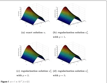
Figure 1 ε= 1×10–3,k= 0.5

By the technique of separation of variables, we can obtain the solution to the direct problem (3.1) as follows:

u(x,y) = ∞

n=1

ϕnsin(nx)cosh

√

k2_+n2_{y, (3.2)}

whereϕn=_πcosh(2_k2_+n2₎dn,dn=

π

0 x(π–x)(1 +x)sin(nx)dx, which can be computed by

employing the Simpson formulation.

Next, the initial dataϕ(x) is chosen as follows:

ϕ(x) =u(x, 0)≈

25

n=1

ϕnsin(nx). (3.3)

We give the measured dataϕδ_(x

i) =ϕ(xi) +εrand(i), whereεis an error level and

δ:=ϕδ–ϕl2=

1 N1

N1

i=1

ϕδ(xi) –ϕ(xi)

2 1/2

. (3.4)

The functionrand(·) denotes a random number uniformly distributed in the interval [0, 1]. The relative root mean square error between the exact and regularization solution is given by

(u) =

1

N1×N2

N1 i=1

N2

j=1(u(xi,yj) –uδα(xi,yj))2

1

N1×N2

N1 i=1

N2

j=1(u(xi,yj))2

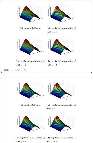
Figure 2 ε= 1×10–2_{,k= 0.5}

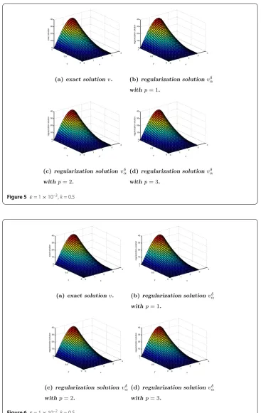
Figure 3 ε= 1×10–3_{,k= 1.2}

where

xi= (i– 1) N1– 1

π, yj= (j– 1) N2– 1

Figure 4 ε= 1×10–2,k= 1.2

Table 1 k= 0.5, the relative root mean square errors(u) for various noise levels

ε 0.0001 0.001 0.005 0.01 0.05

p= 1 0.0014 0.0037 0.0117 0.0270 0.0814

p= 2 0.0025 0.0073 0.0205 0.0344 0.1184

p= 3 0.0046 0.0129 0.0311 0.0492 0.1323

Table 2 k= 1.2, the relative root mean square errors(u) for various noise levels

ε 0.0001 0.001 0.005 0.01 0.05

p= 1 0.0018 0.0056 0.0212 0.0394 0.1581

p= 2 0.0032 0.0113 0.0394 0.9705 0.2479

p= 3 0.0060 0.0203 0.0637 0.1075 0.3240

In the numerical computations, we only consider the cases whenp= 1, 2, 3, and always takeN1=N2= 31. We choose the regularization parameterαby (2.14).

We have shown the numerical results in Figs.1–4and Tables1–2. The numerical re-sults foru(·,y) anduδ

α(·,y) withk= 0.5 andε= 0.001, 0.01 are respectively shown in Fig.1 and Fig.2. The numerical results foru(·,y) anduδ

Example2 The following direct problem for the modified Helmholtz equation is consid-ered:

⎧ ⎪ ⎪ ⎪ ⎪ ⎪ ⎨ ⎪ ⎪ ⎪ ⎪ ⎪ ⎩

vxx+vyy–k2v= 0, 0 <x<π, 0 <y< 1,

v(x, 0) = 0, 0≤x≤π,

vy(x, 1) =x(π–x), 0≤x≤π,

v(0,y) =v(π,y) = 0, 0≤y≤1,

(3.7)

whereT= 1.

By the technique of separation of variables, we get the solution to the direct problem (3.7) as follows:

v(x,y) = ∞

n=1

2

πsinh(√k2_+n2₎

π

0

x(π–x)sin(nx)dxsin(nx)sinh√k2_+n2_{y. (3.8)}

Then

vy(x,y) =

∞

n=1

ψnsin(nx)cosh

√

k2_+n2_{y, (3.9)}

whereψn=_πsinh2_(kn2_+n2₎en,en=

π

0 x(π–x)sin(nx)dx.

We give the initial data

ψ(x) =vy(x, 0)≈

20

n=1

ψnsin(nx) (3.10)

and the measured dataψδ_(x

i) =ψ(xi) +εrand(i), whereεis an error level.

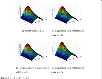
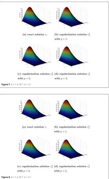
We have shown the numerical results in Figs.5–8and Tables3–4. The numerical re-sults forv(·,y) andvδ

α(·,y) withk= 0.5 andε= 0.001, 0.01 are respectively shown in Fig.5 and Fig.6. The numerical results forv(·,y) andvδ

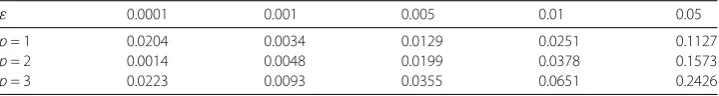
α(·,y) withk= 1.2 andε= 0.001, 0.01 are respectively shown in Fig.7and Fig.8. The relative root mean square errors for the com-puted solution versus the error levelsεare respectively shown in Table3 (k= 0.5) and Table4(k= 1.2).

By Figs.1–8 and Tables1–4, we observe that our proposed method is effective and stable. From Tables1–2and3–4, we note that the smallerεis, the better the calcula-tion effect is, which means that our proposed regularizacalcula-tion method is convergent with respect to decreasing the noise level ε. In addition, from Tables1to4, we can see the relative root mean square errors(u) = 0.0014 and(v) = 0.0313 for various noise levels whenk= 0.5,ε= 0.0001,p= 1, and the relative root mean square errors(u) = 0.0018 and

Figure 5 ε= 1×10–3,k= 0.5

Figure 6 ε= 1×10–2,k= 0.5

4 Conclusions

Figure 7 ε= 1×10–3_{,k= 1.2}

Figure 8 ε= 1×10–2_{,k= 1.2}

Table 3 k= 0.5, the relative root mean square errors(v) for various noise levels

ε 0.0001 0.001 0.005 0.01 0.05

p= 1 0.0313 0.0040 0.0096 0.0183 0.0815

p= 2 0.0019 0.0043 0.0129 0.0223 0.0850

p= 3 0.0029 0.0084 0.0226 0.0367 0.1206

Table 4 k= 1.2, the relative root mean square errors(v) for various noise levels

ε 0.0001 0.001 0.005 0.01 0.05

p= 1 0.0204 0.0034 0.0129 0.0251 0.1127

p= 2 0.0014 0.0048 0.0199 0.0378 0.1573

p= 3 0.0223 0.0093 0.0355 0.0651 0.2426

case and the proofs are similar. It should be mentioned that the method of separation of variables is used to give the expression of solution, so the proposed method in this paper can be extended to solve the Cauchy problems of Helmholtz-type equation in a cylindrical domain. But it cannot be applied in more general geometries, which is a limit of the non-local boundary value problem method.

Acknowledgements

This work was supported by the Natural Science Foundation of China (No. 61763044) and the Natural Science Foundation of Gansu Province (No. 18JR3RA096). The authors are very grateful to the anonymous referees for their valuable suggestions.

Funding Not applicable.

Abbreviations Not applicable.

Availability of data and materials Not applicable.

Competing interests

All of the authors of this article claim that together they have no competing interests.

Authors’ contributions

HY and QYY completed the main study together. HY wrote the manuscript, QYY checked the proofs process and verified the calculation. Moreover, all the authors read and approved the last version of the manuscript.

Publisher’s Note

Springer Nature remains neutral with regard to jurisdictional claims in published maps and institutional affiliations.

Received: 17 April 2018 Accepted: 20 September 2018 References

1. Cheng, H.W., Huang, J.F., Leiterman, T.J.: An adaptive fast solver for the modified Helmholtz equation in two dimensions. J. Comput. Phys.211(2), 616–637 (2006)

2. Juffer, A.H., Botta, E.F.F., Van Keulen, B.A.M., Ploeg, A.V.D., Berendsen, H.J.C.: The electric potential of a macromolecule in a solvent: a fundamental approach. J. Comput. Phys.97(4), 144–171 (1991)

3. Liang, J., Subramaniam, S.: Computation of molecular electrostatics with boundary element methods. Biophys. J.

73(4), 1830–1841 (1997)

4. Russel, W.B., Saville, D.A., Schowalter, W.R.: Colloidal Dispersions. Cambridge University Press, Cambridge (1991) 5. Li, X.: On solving boundary value problems of modified Helmholtz equations by plane wave functions. J. Comput.

Appl. Math.195(1), 62–82 (2006)

6. Yoneta, A., Tsuchimoto, M., Honma, T.: Analysis of axisymmetric modified Helmholtz equation by using boundary element method. IEEE Trans. Magn.26(2), 1015–1018 (1990)

7. Lin, J., Chen, C.S., Liu, C.S.: Fast solution of three-dimensional modified Helmholtz equations by the method of fundamental solutions. Commun. Comput. Phys.20(2), 512–533 (2016)

9. Lin, J., Chen, W., Wang, F.: A new investigation into regularization techniques for the method of fundamental solutions. Math. Comput. Simul.81(6), 1144–1152 (2011)

10. Goubet, O., Hamraoui, E.: Blow-up of solutions to cubic nonlinear Schrödinger equations with defect: the radial case. Adv. Nonlinear Anal.6(2), 183–197 (2017)

11. Kumar, S., Kumar, D., Singh, J.: Fractional modelling arising in unidirectional propagation of long waves in dispersive media. Adv. Nonlinear Anal.5(4), 383–394 (2016)

12. Hadamard, J.: Lectures on Cauchy’s Problem in Linear Partial Differential Equations. Dover Publications, New York (1953)

13. Tikhonov, A.N., Arsenin, V.Y.: Solutions of ill-posed problems New York (1977)

14. Isakov, V.: Inverse Problems for Partial Differential Equations, vol. 127. Springer, New York (1998)

15. Marin, L., Elliott, L., Heggs, P.J., Ingham, D.B., Lesnic, D., Wen, X.: Conjugate gradient boundary element solution to the Cauchy problem for Helmholtz-type equations. Comput. Mech.31, 367–377 (2003)

16. Marin, L., Elliott, L.: BEM solution for the Cauchy problem associated with Helmholtz-type equations by the Landweber method. Eng. Anal. Bound. Elem.28, 1025–1034 (2004)

17. Wen, D.W., Qin, H.H.: Tikhonov type regularization method for the Cauchy problem of the modified Helmholtz equation. Appl. Math. Comput.203(2), 617–628 (2008)

18. Marin, L., Lesnic, D.: The method of fundamental solutions for the Cauchy problem associated with two-dimensional Helmholtz-type equations. Comput. Struct.83, 267–278 (2005)

19. Wei, T., Hon, Y.C.: Solving Cauchy problems of elliptic by the method of fundamental solutions in boundary elements xxvii. WIT Trans. Model. Simul.39, 57–65 (2005)

20. Wei, T., Hon, Y.C., Ling, L.: Method of fundamental solutions with regularization techniques for Cauchy problems of elliptic operators. Eng. Anal. Bound. Elem.31(4), 373–385 (2007)

21. Qin, H.H., Wei, T.: Quasi-reversibility and truncation methods to solve a Cauchy problem for the modified Helmholtz equation. Math. Comput. Simul.80(2), 352–366 (2009)

22. Hao, D.N.N., Duc, V., Sahli, D.: A non-local boundary value problem method for the Cauchy problem for elliptic equations. Inverse Probl.25, 055002 (2009)

23. Denche, M., Bessila, K.: A modified quasi-boundary value method for ill-posed problems. J. Math. Anal. Appl.301(2), 419–426 (2005)

24. Hao, D.N.N., Duc, V., Sahli, H.: A non-local boundary value problem method for parabolic equations backward in time. J. Math. Anal. Appl.345(2), 805–815 (2008)

25. Melnikova, I.V.: Regularization of ill-posed differential problems. Sib. Mat. Zh.33(2), 125–134 (1992)

26. Trong, D.D., Tuan, N.H.: A nonhomogeneous backward heat problem: regularization and error estimates. Electron. J. Differ. Equ.2008, 33 (2008)

27. Showalter, R.E.: Cauchy problem for hyper-parabolic partial differential equations. In: Trends in the Theory and Practice of Non-Linear Analysis (1983)