R E S E A R C H
Open Access
Green’s function for the boundary value
problem of the static Klein-Gordon equation
stated on a rectangular region and its
convergence analysis
Hao Cheng
1,2*, Xiyu Mu
3, Hua Jiang
2, Guoqing Liu
2and Ming Wei
1*Correspondence: [email protected] 1Collaborative Innovation Center on Forecast and Evaluation of Meteorological Disasters, Nanjing University of Information Science & Technology, No. 219 Ningliu Road, Nanjing, 210044, China
2College of Mathematics & Physics, Nanjing Tech University, No. 30 Puzhu Road(S), Nanjing, 211816, China
Full list of author information is available at the end of the article
Abstract
This study is motivated by solving the inverse boundary problem of the static
Klein-Gordon equation (SKGE), which usually occurs in data assimilation problems. For the purpose of obtaining boundary conditions, thepro formasolution of the problem is provided by using Green’s function. The representation in double series of Green’s function for the SKGE on a rectangular region is obtained by means of the method of images. Convergence analysis shows that the representation is uniformly convergent, which is computer friendly, and can be applied to approximate computations.
MSC: 26B20; 35J08
Keywords: Green’s function; Klein-Gordon equation; inverse problem; boundary value problem; rectangular region
1 Introduction
This research is motivated by solving the inverse boundary value problem of the static Klein-Gordon equation (SKGE), which is formulated from data assimilation. Data assim-ilation is the process by which observations of the actual system are incorporated into the model state of a numerical model of that system. Applications of data assimilation arise in many fields of geosciences, most importantly in weather forecasting and hydrology []. Data assimilation can be transferred into a variational problem, whose corresponding Eu-ler equation is an elliptic PDE, such as a SKGE. These data assimilation problems have some specific features: the boundary conditions are unknown, and some parameters, such as weighted coefficients, are unknown. In general, such problems are known in the liter-ature as inverse problems. There exists much work on the identification problem of pa-rameter estimation [–]. However, the problem of estimating the boundary conditions from observations of the solution has, to the best of our knowledge, seldom been studied in the literature. We could find in the literature only little related work. A class of in-verse problems for the Laplace equation involves estimating the boundary function based on some values of the interior points using a linear assumption as regards the boundary function []. In [], the inverse boundary value problem of determining three dimensional
unknown inclusions was considered. In paper [], the authors obtain essentially best pos-sible stability estimates for a class of inverse problems associated to elliptic boundary value problems. Three examples of vibrating systems were considered whose mathematical de-scriptions lead to the Klein-Gordon equation in []. In paper [], P-C scheme based on the use of rational approximants of second order to the matrix exponential term in a three-time level recurrence relation is applied to the nonlinear Klein-Gordon equation. But to estimate the boundary conditions from observations of the solution, to the best of our knowledge, the mentioned inverse boundary problem has seldom been studied in the literature. We could find in the literature only little related work.
Since most inverse problems are ill-posed, many popular techniques for solving inverse problems use some sort of numerical optimization. The unknown parameters or bound-ary conditions are chosen to be those that best agree with the observed data according to some criterion. In general, assume that the observed data and the desired parameters are related by a mathematical model, such as a differential equation, and that the data can be simulated for any appropriate estimate of the parameters or properly assumed bound-ary conditions. The output least-squares method is very natural: choose values for the parameters, simulate the data, compare them with the observed data, and then measure the misfit. Intuitively, if the formal solution of the PDE of the SKGE is provided, then the inverse problem can easily be formed as a model of approximation. This leads to the fol-lowing questions: Can we explicitly solve the boundary problems for the SKGE? If so, can we construct computer-friendly representations?
In [], the authors studied the Green’s functions for the SKGE. The method of images was applied to various boundary value problems in some unbounded domains, includ-ing the infinite strip, the infinite circular sector and the half-plane. The correspondinclud-ing Green’s functions for the SKGE were constructed in a rapidly convergent series represen-tation, which is a suitable form for the numerical implementation of Green’s functions. The method of eigenfunction expansion was used for constructing the Green’s functions of the boundary value problems in the unbounded domain, such as the infinite strip. The corresponding series of Green’s functions converges uniformly and can be accurately com-puted by a direct truncation. However, the series of Green’s functions for the rectangle is not computer friendly, as it is not uniformly convergent. To address this issue, in [, ], the author provided explicit formulas for the Green’s function of an elliptic PDE in the half-plane and the infinite strip, which were expressed in elementary and special function forms by means of Fourier transformations. However, the construction of Green’s function in [] cannot be adapted to obtain the explicit Green’s function on rectangular regions, as the Fourier transformation requires an infinite domain.
In this paper, we discuss a method of solving the elliptic equation on a rectangular re-gion. A computer-friendly representation of Green’s function for the Static Klein-Gordon Equation is obtained by the method of images. Convergence analysis shows that the rep-resentation can be used for approximate computation.
2 The variation formulas and the corresponding inverse boundary value problem
Consider a variational model in data assimilation as follows: Assume thatuRis the remote
sensing observed value. Let us fixuGas the sensing data of some other sensorGin the same
observation field, usually more accurate and distributed over fewer grid points. According to the smoothness and the dependence on the observation, an unknown functionu(x,y) is set up to satisfy the following functional extremum problem:
I(u) =
∂u
∂x
+
∂u
∂y
+μR(u–uR)+μG(u–uG)
dx dy=min, ()
where represents a special region in two-dimensional Euclidean space, and the non-negative quantitiesμR,μG are weighted coefficients. The first derivative of equation ()
expresses smoothness, and the subtracted part expresses observation error. In addition, the values ofu(x,y) on the boundaryof regionare given by
u(x,y)|=g(x,y). ()
This is a functional extremum problem with a boundary constraint. Its corresponding Euler’s equation and its boundary conditions are presented as follows:
∂u
∂x +
∂u
∂y –μu=μ
u, ()
u(x,y)|=g(x,y), ()
whereμu=μRuR+μGuG.
Obviously, this is a typical Dirichlet problem stated on a special region for an elliptic equation. Generally, it admits a unique classical solution.
Unfortunately, unknown boundary conditions are a very common problem with data assimilation, so we cannot directly solve the above problem. In practice, one can as-sume the boundary conditions, which results in large errors, as the solution of an ellip-tic equation is continuously dependent on the boundary conditions, and there may be a large difference between the assumed boundary conditions and the real boundary condi-tions.
In data assimilation, instead of obtaining with difficulty the values on the boundary, we easily observe the values ofu(x,y) in sub-region, that is,u(x,y) =u˜(x,y), (x,y)∈⊂. We try to obtain the boundary conditions from the interior observationu˜(x,y). This is obviously an inverse problem. To solve this problem, intuitively, one can obtain the ex-pression of the solution to equations () and () and then evaluate the unknown boundary conditions to minimize the deviation between the solution and the actual observed values. It is well known that elliptic equations can be solved using Green’s functions. In fact, according to the Green’s function method, the formal solution of the elliptic equation in the Dirichlet problem presented in () and () is given as follows:
u(ξ,η) =
G(x,y;ξ,η)f(x,y)dx dy+
g∂G
where G(x,y;ξ,η) is known as Green’s function, andf(x,y) =μu. With the help of the formal solution above, we can setu–u˜=minto findg. Obviously, it is important to find an explicit solution when obtaining the boundary conditions. In this paper, we focus on the construction of a computer-friendly Green’s function and its convergence for approximate computation.
3 Green’s function for the SKGE stated on a rectangular region
In the following paragraph of this paper, we address the elliptic two-dimensional static Klein-Gordon equation (SKGE),
∇u(P) –ku(P) = , ()
where∇is the Laplace operator in the coordinates of the pointPandkis a real constant
parameter. The homogeneous boundary value problem
Miu(p)≡αi(P)
∂u(P) ∂ni
+βi(P)u(P) = , P∈i ()
is set up for the nonhomogeneous equation
∇u(P) –ku(P) = –f(P), P∈, ()
whererepresents a connected region in two-dimensional Euclidean space. In this paper, we focus on dealing with the SKGE on a rectangular region, whose boundary is=∪
∪∪, with
=
(x,y)|≤x≤a,y= , =
(x,y)|≤y≤b,x=a, =
(x,y)|≤x≤a,y=b, and
=
(x,y)|≤y≤b,x= .
It is well known that the solution to the boundary value problem, () and (), can be expressed as follows:
u(P) =
G(P,Q)f(Q)d(Q). ()
In the above representation, the kernelG(P,Q) is said to be the Green’s function for the homogeneous problem corresponding to that of () and ().PandQin () are referred to as the field point and the source point, respectively.
For any source pointQ∈, the corresponding Green’s function, as a function of the coordinates of the field pointP, can be expressed as [, , ]
G(P,Q) = πK
whereK(k|P–Q|) is the modified cylindrical Bessel function of the second kind of order
zero, and R(P,Q) satisfies the homogeneous SKGE everywhere on , regardless of the relative locations ofPandQ. The singular component πK(k|P–Q|) is the response at a
field pointPto a unit source placed at an arbitrary pointQ. In the method of images, the regular componentR(P,Q) ofG(P,Q) is expressed as a sum of a number of unit sources and sinks placed at pointsQ∗,Q∗, . . . ,Q∗moutside the region. It yields the regular component
R(P,Q) =
m
j= ∓K
kP–Q∗j ()
ofG(P,Q), a function satisfying the homogeneous SKGE at any pointPin.
As in paper [], it is easy to construct Green’s function for the SKGE on the upper half-plane={(x,y)|–∞<x<∞,y> }. In fact, the influence of the unit source at a point
Q(ξ,η)∈γ represents the singular component
πK
k(x–ξ)+ (y–η) ()
of the Green’s function. It can be compensated with a single unit sink placed at point
Q∗(ξ, –η) located in the lower half-plane and symmetric toQ(ξ,η) about the boundary
y= . The Green’s function for the upper half-plane is found to be
G(x,y;ξ,η) = π
K
k|z–ζ|–K
k|z–ς¯|. () The Green’s function of the Dirichlet problem for the SKGE on the infinite strip =
{(x,y)|–∞ ≤x≤ ∞, ≤y≤b}is presented as
˜
G+(x,y;ξ,η) = π
∞
n=–∞
K
k(x–ξ)+ (y–η+ nb)
–K
k(x–ξ)+ (y+η– nb). ()
To derive the Green’s function stated on the rectangular region ={(x,y)|≤x≤a, ≤y≤b}, we similarly use the method of images in the following paragraph.
Obviously,G˜+(x,y;ξ,η) satisfies the Dirichlet conditions on the boundary fragmenty= andy=b. However, it conflicts with the Dirichlet conditions on the boundary fragments
x= andx=a. To construct the Green’s function satisfying all boundary conditions, we consider the compensation that results by introducing new sinks.
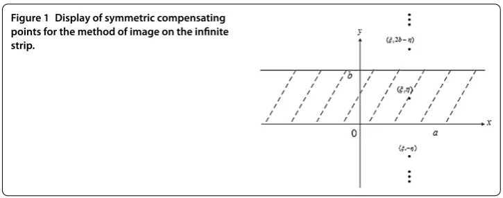
In fact, if we place the unit sources at the point set (Figure )
˜
S+=(ξ, –η), (ξ, b–η), (ξ, –b+η), (ξ, b+η), (ξ, –b–η),
(ξ, b–η), . . . , (ξ,η– nb), (ξ, –η+ nb), . . . () in, then the response toS˜+at field point (x,y) is as follows:
˜
G+(x,y;ξ,η) = π
∞
n=–∞
K
k(x–ξ)+ (y–η+ nb)
–K
Figure 1 Display of symmetric compensating points for the method of image on the infinite strip.
and it is not difficult to show thatG˜+(x,y;ξ,η) satisfies the Dirichlet conditions on the boundary fragmentsy= andy=b but conflicts with the Dirichlet conditions on the boundary fragmentsx= andx=a. Similar to the above discussion, the trace of the so-lutionG˜+(x,y;ξ,η) on the boundary linex= can be compensated for with the unit sinks
˜
S+,=(–ξ, –η), (–ξ, b–η), (–ξ, –b+η), (–ξ, b+η), (–ξ, –b–η),
(–ξ, b–η), . . . , (–ξ,η– nb), (–ξ, –η+ nb), . . . () which represent the images ofS˜+
aboutx= . The response to these sinks at (x,y) evidently
isG˜–
,(x,y;ξ,η) = –πG˜
+
(x,y; –ξ,η).
To compensate for the trace ofG˜+
(x,y;ξ,η) onx=a, we place a series unit sinks ˜
S+a,=(a–ξ, –η), (a–ξ, b–η), (a–ξ, –b+η), (a–ξ, b+η), (a–ξ, –b–η),
(a–ξ, b–η), . . . , (a–ξ,η– nb), (a–ξ, –η+ nb), . . . () which represent the images ofS˜+about the linex=a. The response to these sinks at (x,y) evidently is
˜
G–a,(x,y;ξ,η) = – πG˜
+
(x,y; a–ξ,η). ()
The functionsG˜–
,(x,y;ξ,η) andG˜a–,(x,y;ξ,η) do not vanish on the boundary linesx=
andx=a, and their traces can be properly compensated for by the set of unit sources
˜
S+,=(–a+ξ, –η), (–a+ξ, b–η), (–a+ξ, –b+η), (–a+ξ, b+η), (–a+ξ, –b–η), (–a+ξ, b–η), . . . ,
(–a+ξ,η– nb), (–a+ξ, –η+ nb), . . . () and
˜
S+a,=(a+ξ, –η), (a+ξ, b–η), (a+ξ, –b+η), (a+ξ, b+η), (a+ξ, –b–η), (a+ξ, b–η), . . . ,
The responses to these at (x,y) are given as
˜
G+,(x,y; –a+ξ,η) = πG˜
+
(x,y; –a+ξ,η) ()
and
˜
G+
a,(x,y; a+ξ,η) =
πG˜
+
(x,y; a+ξ,η). ()
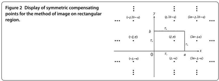
Upon following the above described procedure, we properly place compensatory unit sources that alternate with compensatory unit sinks as follows:
˜
S+,=(–a–ξ, –η), (–a–ξ, b–η), (–a–ξ, –b+η), (–a–ξ, b+η), (–a–ξ, –b–η), (–a–ξ, b–η), . . . ,
(–a–ξ,η– nb), (–a–ξ, –η+ nb), . . ., ()
˜
S+a,=(a–ξ, –η), (a–ξ, b–η), (a–ξ, –b+η), (a–ξ, b+η), (a–ξ, –b–η), (a–ξ, b–η), . . . ,
(a–ξ,η– nb), (a–ξ, –η+ nb), . . . () ..
.
˜
S+,n=(–na+ξ, –η), (–na+ξ, b–η), (–na+ξ, –b+η), (–na+ξ, b+η), (–na+ξ, –b–η), (–na+ξ, b–η), . . . ,
(–na+ξ,η– nb), (–na+ξ, –η+ nb), . . ., ()
˜
S+a,n=(na+ξ, –η), (na+ξ, b–η), (na+ξ, –b+η), (na+ξ, b+η), (na+ξ, –b–η),
(na+ξ, b–η), . . . , (na+ξ,η– nb), (na+ξ, –η+ nb), . . ., ()
˜
S+,n+=(–na–ξ, –η), (–na–ξ, b–η), (–na–ξ, –b+η), (–na–ξ, b+η), (–na–ξ, –b–η), (–na–ξ, b–η), . . . ,
(–na–ξ,η– nb), (–na–ξ, –η+ nb), . . ., ()
˜
S+a,n+=(n+ )a–ξ, –η,(n+ )a–ξ, b–η,
(n+ )a–ξ, –b+η,(n+ )a–ξ, b+η,
(n+ )a–ξ, –b–η,(n+ )a–ξ, b–η, . . . ,
(n+ )a–ξ,η– nb,(n+ )a–ξ, –η+ nb, . . . () ..
.
Figure 2 Display of symmetric compensating points for the method of image on rectangular region.
Hence, we express the Green’s functionG(x,y;ξ,η) stated on a rectangular region in the form
G(x,y;ξ,η) =G˜+(x,y;ξ,η) +
∞
n= ˜
G–,n–+G˜–a,n–+
∞
n= ˜
G+,n+G˜+a,n. ()
After a trivial substitution, the Green’s function of the SKGE stated on a rectangular region can be expressed as the double infinite series
G(x,y;ξ,η) = π
∞
n=–∞ ∞
m=–∞
K
k(x–ξ+ ma)+ (y–η+ nb)
–K
k(x–ξ– ma)+ (y+η– nb). () 4 Convergence of the double infinite series of Green’s function
Since the Green’s function in () is expressed as a double infinite series, its convergence ought to be specifically addressed to ensure its computability. Note first that the singularity in () is provided by the component that is a part of a simple term (m= ,n= ), which does not, in any way, affect the convergence.
First, we note that the logarithmic singularity in
K(x) = –
C+lnx
∞
j=
xj
j(j!) + ∞
m=
xm
m(m!) m
n=
n
, ()
with Euler’s constantC≈., is provided by the component that is a part of a single term (m= ,n= ) and cannot affect the series convergence.
To study the convergence of the series (), we consider the asymptotic property of Mac-donald’s functionK(x) asxtends to infinity.
4.1 The asymptotic property of Macdonald’s function
K(x) is Neumann’s Bessel function of the second kind of order zero:
K(x) =J(x)logx+
x
– x
+· · ·, ()
where
J(x) = –
x
+
x
·–
x
For the purpose of studying the asymptotics ofK(x), we need to use the following
rela-tion []:
Kn(z) =
π z
cosnπW,n(z), ()
where
Wk,m(z) = –
πi
k+ –m
e–zzk
(+)
∞ (–t) –k–+m
+t
z
k–+m
e–tdt ()
is the solution of the following equation:
dW dz +
– + k z+ –m
z
W= . ()
It is easy to show that
Wk,m(z) =e–
zzk
+m
– (k– )
!z +
{m– (k–)}{m– (k–)} !z +· · ·
+{m
– (k– )
}{m– (k– )
} · · · {m– (k–n+ )
}
n!zn
+
(–k++m)
∞
t–k–+mR
n(t,z)e–tdt
()
withRn(t,z) = λ(λ–)···(n! λ–n)( + tz)λ
t/z
un( +u)–
λ–du.
When|z|> , we have
(–k+ +m)
∞
t–k–+mR
n(t,z)e–tdt
=Oz–n–. ()
The constant implied in the symbol O is independent ofarg(z), and the expansion of
Wk,m(z) is
Wk,m(z) =e–
zzk
+m
– (k– )
!z +
{m– (k–
)}{m– (k– )}
!z +· · ·
+{m
– (k–
)}{m– (k–
)} · · · {m– (k–n+ )}
n!zn
+Oz–n–. ()
Ifk= ,m= , we have
W,(z) =e–
z +–( )
!z +
{()}{( )}
!z +· · ·
+(–)
n{( )}{(
)} · · · {(n– )}
n!zn +O
Whennis an integer,Kn(z) is defined as
Kn(z) = – ∞
r=
(z)n+r
r!(n+r)!
logz
+γ –
n+r
m=
m–– r m= m– + n– r= z
–n+r
(–)n–r(n–r– )!
r! , ()
whereγ ∼= . is Euler’s constant. Whenn= andxis real, we have
K(x) =
π x
W,(x) =
π x
e–x
+–(
)
!x +
{()}{( )}
!(x) +· · ·
+(–)
n{( )
}{( )
} · · · {(n– )
}
n!(x)n +O
x–n–. ()
It is obvious that whenxis sufficiently large, the above relation can be rewritten as
K(x) =
π x
e–x
+O
|x|
. ()
4.2 Convergence of double series
As the Green’s function is represented in the form of a double infinite series, for the pur-pose of approximate computation, we now summarize some definitions and results about the uniform convergence of the series.
Definition The infinite setai,j,i= , , . . . ;j= , , . . . can be arranged in the shape of an
infinite matrix,
a, a, a, · · ·
a, a, a, · · ·
a, a, a, · · · · · · ·
Adding up all these elements, we obtain a double series,∞i=∞j=ai,j, called the iterated
series. LetSm,n=
m i=
n
j=ai,jdenote a double series subtotal. Whenlimm→∞
n→∞ Sm,n=Sand
Shas a limited value, the double series is defined as a convergent series.
Theorem Suppose that≤ |ai,j| ≤bi,j;if
∞
i=
∞
j=bi,jconverges,then
∞
i=
∞
j=ai,j
ab-solutely converges.
Theorem Suppose the function series∞m=n∞=um,n(x,y), (x,y)∈and∃m,n∈Z+,
(x,y) ∈ ; if |um,n(x,y)| ≤ am,n(x,y) and
∞
m=
∞
n=am,n(x,y) converges, then
∞
m=
∞
4.3 The convergence of infinite double series of Green’s function
To study the uniform convergence of the double series, we need to construct its dominant series. We discuss the common term of the series
amn(x,y) =K
k(x– ma+ξ)+ (y–η+ nb)
–K
k(x– ma+ξ)+ (y+η+ nb), ()
where the subtraction of the two terms in its general formula physically represents the electric potential at point (x,y) from point charges at two points (ma–ξ,η+ nb), (ma– ξ,η– nb). Since the potential of every term for largem,nis sufficiently small, by ignoring their offsetting effect, we can estimate them item by item.
Whenm,nare large enough, it is not difficult to show that
lim
n→∞ m→∞
(x–ξ+ ma)+ (y–η+ nb)
(ma)+ (nb) = .
We define
α=(x–ξ+ ma)+ (y–η+ nb)= (ma)+ (nb)+O() ()
asm,n→ ∞. Consequently, whenm,nare sufficiently large, from () and (), we have
K
k(x–ma+ξ)+ (y–η+ nb)
=
π αk
e–αk
+O
|α|
=
π
k(ma)+ (nb)
e–k
√
(ma)+(nb)
+O
|m|+|n|
. ()
Similarly,
K
k(x–ma+ξ)+ (y+η+ nb)
=
π
k(ma)+ (nb)
e–k
√
(ma)+(nb)
+O
|m|+|n|
. ()
Hence,
amn(x,y)≤K
k(x–ma+ξ)+ (y–η+ nb)
+K
k(x–ma+ξ)+ (y+η+ nb) ≤
√
π/k
(ma)+ (nb)e
–k√(ma)+(nb)
+O
|m|+|n|
It is easy to show that the double series∞n=–∞∞m=–∞
√
π/k
√
(ma)+(nb)e
–k√(ma)+(nb)
is
absolutely convergent. Hence,
G(x,y;ξ,η) = π
∞
n=–∞ ∞
m=–∞
K
k(x–ξ+ ma)+ (y–η+ nb)
–K
k(x–ξ– ma)+ (y+η– nb) ()
is absolutely uniformly convergent.
Theorem The following is a computer-friendly representation of Green’s function for the static Klein-Gordon equation:
G(x,y;ξ,η) = π
N
n=–N M
m=–M
K
k(x–ξ+ ma)+ (y–η+ nb)
–K
k(x–ξ– ma)+ (y+η– nb)+O
|M|+|N|
. ()
5 Numerical examples
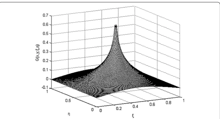
In this section, we give corresponding numerical examples to investigate the performances of the proposed Green’s function ().G(x,y;ξ,η) on the rectangular region (≤ξ≤, ≤η≤) is plotted in Figure for (x,y) = (., .). From the figure, we note thatG= on the boundaryξ = ,ξ= , andG→ ∞as (ξ,η)→(x,y). These are, in fact, general properties of the Green’s function.
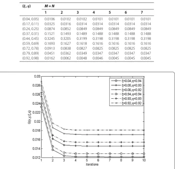
To investigate the convergence performance of the Green’s function (), we select sev-eral points to perform the simulation. Table and Figure show that the Green’s function () converges quickly. All the points converge steadily to their true numerical values after a limited number of iterations.
Table 1 Convergence procedure of nine selected points
(ξ,η) M = N
1 2 3 4 5 6 7
(0.04, 0.05) 0.0106 0.0102 0.0102 0.0101 0.0101 0.0101 0.0101 (0.17, 0.11) 0.0325 0.0316 0.0314 0.0314 0.0314 0.0314 0.0314 (0.24, 0.25) 0.0874 0.0852 0.0849 0.0849 0.0849 0.0849 0.0849 (0.37, 0.31) 0.1521 0.1493 0.1489 0.1488 0.1488 0.1488 0.1488 (0.44, 0.45) 0.3245 0.3205 0.3199 0.3198 0.3198 0.3198 0.3198 (0.59, 0.69) 0.1693 0.1627 0.1618 0.1616 0.1616 0.1616 0.1616 (0.72, 0.78) 0.0913 0.0838 0.0827 0.0825 0.0825 0.0825 0.0825 (0.79, 0.89) 0.0451 0.0362 0.0349 0.0347 0.0347 0.0347 0.0347 (0.92, 0.98) 0.0162 0.0062 0.0048 0.0046 0.0045 0.0045 0.0045
Figure 4 Convergence trend of the six arbitrary points.
6 Conclusions
In this paper, we consider the boundary value problem for the static Klein-Gordon equa-tions, which are associated with the Euler equation from data assimilation applications. In real application problems, such as data assimilations, the rectangle is the most popular analysis region. The present study focuses formally on solving the elliptic Klein-Gordon equation on a rectangular region, which can be used for obtaining the boundary con-ditions by numerical optimization. Green’s function for the static Klein-Gordon equa-tion is constructed through the method of images. Convergence analysis shows that the computer-friendly representation can be used for numerical computation.
Competing interests
The authors declare that they have no competing interests.
Authors’ contributions
The authors have equally made contributions to each part of this paper. All authors read and approved the final manuscript.
Author details
Acknowledgements
The article was supported by the National Natural Science Foundation of China (No. 61401236).
Publisher’s Note
Springer Nature remains neutral with regard to jurisdictional claims in published maps and institutional affiliations.
Received: 16 February 2017 Accepted: 2 May 2017 References
1. Talagrand, O, Courtier, P: Variational assimilation of meteorological observations with the adjoint vorticity equation. I: Theory. Q. J. R. Meteorol. Soc.113, 1311-1328 (1987)
2. Al-Jamal, MF: Numerical solution of elliptic inverse problems via the equation error method. PhD Dissertation, Michigan Technological University (2012)
3. Mehraliyev, YT Kanca, F: An inverse boundary value problem for a second order elliptic equation in a rectangle. Math. Model. Anal.19(2), 241-256 (2014)
4. Mehraliyev, YT: On solvability of an inverse boundary value problem for a fourth order elliptic equation. J. Math. Syst. Sci.3, 560-566 (2013)
5. Orlovsky, DG: Inverse problem for elliptic equation in Banach space with Bitsadze-Samarsky boundary value conditions. J. Inverse Ill-Posed Probl.21, 141-157 (2013)
6. Zhao, S, Wang, Y: The generalized Green’s function of Neumann boundary value problem for the 2th order elliptic equation on a rectangle inR2. Natur. Sci. J. Harbin Normal Univ.3, 1-4 (2003) (in Chinese)
7. Wu, X, Jiang, E, Hou, W: A class of inverse problem for Laplacian equation. J. Shanghai Univ. Nat. Sci.10, 516-520 (2004) (in Chinese)
8. Kim, S: An inverse boundary value problem of determining three dimensional unknown inclusions in an elliptic equation. J. Inverse Ill-Posed Probl.14(9), 881-889 (2006)
9. Alessandrini, G, Beretta, E, Rosset, E, et al.: Inverse boundary value problems with unknown boundaries: optimal stability. Comptes Rendus de l’Académie des Sciences-Series IIB-Mechanics328(8), 607-611 (2000)
10. Gravel, P, Cauthier, C: Classical applications of the Klein-Gordon equation. Am. J. Phys. Teach.79(5), 447-453 (2011) 11. Bratsos, AG: On the numerical solution of the Klein-Gordon equation. Numer. Methods Partial Differ. Equ.25(4),
939-951 (2008)
12. Melnikov, YA: Construction of Green’s functions for the two-dimensional static Klein-Gordon equation. J. Partial Differ. Equ.24(2), 114-139 (2011)
13. Muravey, D: The boundary value problem for a static 2D Klein-Gordon equation in the infinite strip and in the half-plane. Math.40(2), 205-227 (2015)
14. Aseeri, S, Batrasev, O, Icardi, M, et al.: Solving the Klein-Gordon equation using Fourier spectral methods: a benchmark test for computer performance. In: Proceedings of the Symposium on High Performance Computing (HPC’15), pp. 182-191 (2015)
15. Polidoro, S, Ragusa, MA: Harnack inequality for hypoelliptic ultraparabolic equations with a singular lower order term. Rev. Mat. Iberoam.24(3), 1011-1046 (2008)
16. Polidoro, S, Ragusa, MA: Holder regularity for solutions of ultraparabolic equations in divergence form. Potential Anal.
14(4), 341-350 (2001)