R E S E A R C H
Open Access
Approximation on the hexagonal grid of the
Dirichlet problem for Laplace’s equation
Adiguzel A Dosiyev
*and Emine Celiker
*Correspondence:
[email protected] Department of Mathematics, Eastern Mediterranean University, Gazimagusa, K.K.T.C., via Mersin 10, Turkey
Abstract
The fourth order matching operator on the hexagonal grid is constructed. Its application to the interpolation problem of the numerical solution obtained by hexagonal grid approximation of Laplace’s equation on a rectangular domain is investigated. Furthermore, the constructed matching operator is applied to justify a hexagonal version of the combined Block-Grid method for the Dirichlet problem with corner singularity. Numerical examples are illustrated to support the analysis made.
MSC: 35A35; 35A40; 35C15; 65N06; 65N15; 65N22; 65N99
Keywords: Laplace’s equation; Dirichlet boundary value problem; hexagonal grids; matching operator; interpolation for harmonic functions; singularity; Block-Grid method
1 Introduction
When solving PDEs, many approximate methods, such as overlapping versions of domain decomposition, composite grids and different types of combined methods, use the match-ing operator to connect the subsystems within them. Hence, the approximation of the so-lutions relies heavily on the order of accuracy of the matching operator, as well as on the order of accuracy of the subsystems. In [] and [], the second order matching operator is used to construct and justify the second order composite grid method for solving Laplace’s boundary value problems. In [], the fourth order matching operator is constructed and used for the fourth order composite grids and in [] and [] it is used for the fourth or-der Block-Grid method. In [–], the sixth oror-der matching operator is constructed for the Block-Grid method and it is used for the sixth order composite grids in [].
In all of the above mentioned papers, the fourth and sixth order matching operators were constructed on the basis of the -point finite difference solution of Laplace’s equa-tion on square grids. In this paper, the matching operator is constructed for the soluequa-tion of the Dirichlet problem on a hexagonal grid. In order to approximate the given differ-ential equations at each regular nodePon a hexagonal grid, the six equidistant nodes
surroundingPare used, and the truncation error obtained isO(h). Thus, we obtain the
same order of accuracy when using the -point scheme on the hexagonal grid, as we do when using the -point scheme on the rectangular grid (see []). This has many compu-tational advantages such as (i) the matrix of the system will contain seven diagonals rather than nine and will lead to less use of memory space, (ii) the calculations will require less computational effort and (iii) the algorithm will be easier to implement. Hexagonal grids are favored in many applied problems in dynamical meteorology and dynamical
raphy as well (see [–]), due to the benefits a hexagonal grid provides, compared to a rectangular grid.
Even though using a hexagonal grid has the above mentioned advantages, it has not been used before in methods such as composite grids, domain decomposition, and combined methods, as the fourth order matching operator for connecting the subsystems together was not constructed. In this paper, in Section , the approximate solution in a hexagonal grid on a rectangular domain is analyzed. In Section a fourth order matching operator is constructed and its application to find the fourth order accurate approximate solution on the closed domain is considered. Section contains the justification of using a hexagonal grid for the solution of Laplace’s equation on a staircase polygon, with the use of the Block-Grid method. This method requires the application of the matching operator constructed in Section and gives an overall fourth order accuracy. Numerical examples are illustrated in Section to support the analysis made.
2 Approximation in the hexagonal grid of the Dirichlet problem on a rectangle
Let={(x,y) : <x<a, <y<b}be a rectangle,γj,j= , , , , be its sides, including the ends, enumerated counterclockwise starting from left (γ≡γ,γ≡γ),γ =
j=γj be the boundary of, and letAj=γj–∩γjbe thejth vertex. We consider the boundary value problem
u= on, (.)
u=ϕj onγj,j= , , , , (.)
where=∂/∂x+∂/∂y,ϕ
jis a given function of arclengthstaken alongγ, and
ϕj∈C,λ(γj), <λ< ,j= , , , . (.)
At the verticess=sj(sjis the beginning ofγj), the conjugation conditions
ϕj(q)(sj) = (–)qϕj(–q)(sj), q= , , , , (.)
are satisfied.
Leth> , witha/h≥,b/√h≥ integers. We assignha hexagonal grid on, with step sizeh, defined as the set of nodes
h=
(x,y)∈:x=k–j h,y=
√ (k+j)
h,k= , , . . . ;j= ±±, . . .
. (.)
Letγjh be the set of nodes on the interior ofγj, and letγ˙jh=γj∩γj+,γh=
(γjh∪ ˙γjh),
h=h∪γh. Also let∗hdenote the set of nodes whose distance from the boundaryγ ofish andh=h\∗h.
We consider the system of finite difference equations
uh=Suh onh, (.)
uh=ϕj onγjh,j= , , , , (.)
where
Su(x,y) =
u(x+h,y) +u
x+h ,y+
√ h +u
x–h ,y+
√
h
+u(x–h,y) +u
x–h ,y–
√ h +u
x+h ,y–
√
h
, (.)
S∗ju(x,y) =
u
x+h ,y–
√ h
+u(x+h,y)
+u
x+h ,y+
√ h
, (.)
E∗jh(ϕj) =
ϕj
y+ √ h
+ ϕj(y) + ϕj y– √ h . (.)
From formulae (.) and (.) it follows that the coefficients of the expressionsSu(x,y) andSj∗u(x,y) are non-negative, and their sums do not exceed one. Hence, on the basis of the maximum principle, it follows that the solution of system (.)-(.) exists and it is unique (see []).
Everywhere below we will denote constants which are independent ofhand of the cofac-tors on their right byc,c,c, . . . , generally using the same notation for different constants
for simplicity.
Lemma . Let
v=Sv+fh onh,
v=S∗jv on∗h,
v= onγh,
and
v=Sv+fh onh,
v=S∗jv+f
∗
h on∗h,
v=ηh onγh,
where fh,fh,f ∗
handηhare arbitrary grid functions.If the conditions
f∗h≥, |fh| ≤fh, and ηh≥
are satisfied,then
|v| ≤v.
Proof The proof of this lemma is similar to the proof of the comparison theorem (see Ch.
Theorem . Let u be the solution of problem(.), (.)and uhbe the solution of system (.)-(.),then
max
h
|uh–u| ≤ch. (.)
Proof Let
h=uh–u,
whereuis the trace of the solution of problem (.), (.) onh, anduhis the solution of system (.)-(.). Then, the error function hsatisfies the following system:
h=S h+h onh, (.)
h=S∗j h+h∗ on∗h, (.)
h= onγh, (.)
where
h=Su–u, (.)
h∗=S∗ju–u+E∗jh(ϕj) (.)
are the truncation errors of equations (.) and (.), respectively.
On the basis of conditions (.) and (.), from Theorem . in [] it follows thatu∈ C,λ(), <λ< . Then, by Taylor’s formula, we obtain (see [])
max
(x,y)∈
h(x,y)≤chM, (.)
where
Mj= sup
(x,y)∈
∂ju(x,y)
∂xi∂yj–i
,i= , , . . . ,j
.
We represent the solution of (.)-(.) as
h= h+ h, (.)
where
h=S h+h onh,
h=S∗j h on∗h,
h= onγh,
and
h=S∗j h+h∗ on∗h,
h= onγh.
By taking the function asv=hcM(a+b–x–y) in Lemma ., we obtain
max
(x,y)∈h
h≤ max
(x,y)∈|
v| ≤chM. (.)
Using Taylor’s formula about each of the points (h
,y)∈∗hand from (.), we have
max
(x,y)∈∗h
∗≤cMh.
On the basis of the maximum principle, we obtain
max
(x,y)∈h
h≤ (x,maxy)∈∗h
h∗≤cMh. (.)
From (.), (.), and (.) it follows that
max
(x,y)∈h
| h| ≤ch. (.)
Remark . Estimation (.) remains true whenEjh∗(ϕj) in system (.)-(.) is replaced by
E∗j,h= ϕj
y– √
h
+ ϕj
y+ √
h
+
ϕj(y) –
h
!ϕ
()
j (y) +
h
!ϕ
()
j (y).
3 Construction of the fourth order matching operator
Letz=x+iybe a complex variable, and let={z:|z|< }be a unit circle. For a har-monic functionuonwithu∈C,(), by Taylor’s formula, any point (x,y)∈can be represented as
u(x,y) =
k=
akRezk+
k=
bkImzk+Or
, (.)
wherer=x+y,
a=u(, ), a=
∂u(, )
∂x , a=
∂u(, )
∂x , a=
!
∂u(, )
∂x ,
b=
∂u(, )
∂y , b=
∂u(, )
∂x∂y , b=
!
∂u(, ) ∂x∂y .
By analogy with the idea used in [], we construct the operatorSfrom the condition
that the expression
whereuk=u(Pk),Pkis a node of the hexagonal gridh, gives the exact value of any har-monic polynomial
F(x,y) =
k=
akRezk+
k=
bkImzk,
at each pointP∈, and
ξk≥,
ξk≤.
Letdenote the set of pointsP∈such that all the nodesPkto determine the expres-sionSubelong toh, and
contain the pointsP, where some of the nodesPkemerge through the sideγj,j= , , , . We construct the fourth order matching operatorSby considering the cases when the pointPbelongs to one of the setsor.
Case .The pointP∈lies on the line connecting two neighboring grid nodes (a grid
line).
We place the origin of the rectangular system of coordinates on the nodePand direct
the positive axis of xalong the grid line, so thatP=P(δh, ), <δ≤/, and take the nodes.
P(, ), P(h, ), P
h , √ h
, P
–h , √ h , P h , – √ h
, P
–h , – √ h .
First, we find the coefficientsλj,j= , , , , such that the representation
u=λu+λu+λu+λu (.)
is true for the harmonic polynomialsRezn,n= , , , , whereu=u(P),u
k=u(Pk),k= , , , ,z=x+iy. This gives the system
λ+λ+λ+λ= ,
δλ+λ+ λ – λ = ,
δλ+λ– λ – λ = ,
δλ+λ–λ+λ= .
(.)
By solving system (.) and rearranging (.) foru, we obtain the equation
u=u λ–
λ λu–
λ λu–
λ
λu. (.)
We now take into consideration the nodesP(h, –
√
h
) andP(–
h
, –
√
h
) which are
k= , , fory= , and odd with respect toy, andRezk,k= , , , , is even with respect toy, from (.) we have
u=u λ–
λ λu–
λ λu–
λ λu–
λ λu–
λ λu.
Hence, we obtain the matching operatorS, for which the expression
Su=
k=
λkuk (.)
gives the exact value of the harmonic polynomialF(x,y) at the pointP, where
λ= –(– +δ) –δ+δ
, λ=
δ+δ
,
λ=λ=
–(– +δ)δ
, λ=λ=
(– +δ)(–δ+ δ)
.
It is easy to check that
λ> , λj≥, j= , , , for <δ≤/, (.)
and
k=
λk= . (.)
Remark . When / <δ< , the nodeP, which is closest toP, is taken as the origin.
Case. The pointP∈lies inside a grid cell of the hexagonal grid.
Again, we place the origin of the rectangular system of coordinates at the nodePand
direct the positive axis ofxalong the grid line, so thatPhas the coordinatesP(δh, √
hκ
),
where <δ,κ≤/. We form an artificial grid by taking the following points:
P
κh
, √
hκ
, P
h+κh ,
√ hκ
, P
h + κh , √ h + √ hκ
,
P
–h + κh , √ h + √ hκ
, P
h + κh , – √ h + √ hκ
,
P
–h + κh , – √ h + √ hκ
.
Each of the nodesPk,k= , , . . . , , of the artificial grid falls on a grid line, and for the approximation ofPthe expression
Su=
k=
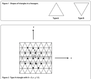
Figure 1 Shapes of triangles in a hexagon.
Figure 2 Type A triangle with 0 <δ,κ≤1/2.
is used. AsPk,k= , , . . . , , all lie on grid lines, each of these points needs to be approxi-mated using the matching operator as follows:
Su=
k=
λkSu Pk
.
From the distribution of the nodes it becomes obvious that only nodes are needed for this approximation (see Figure ).
Hence, we form the matching operator as
Su=
k=
ξku(Pk), (.)
whereξk,k= , . . . , , are defined by the coefficients obtained earlier and
ξk≥,
k=
ξk= . (.)
For the approximation, it is also important to examine the structure of the hexagonal grid. There are two types of triangles in each hexagon,Type AandType B, as shown in Figure .
We consider triangles ofType Awith <δ,κ≤/. The nodes used inSuare shown in
In the case / <δ< , <κ≤/, the nodes used have the same distribution as the reflection of the nodes in Figure about the linex= . In the cases <δ≤/, / <κ< and / <δ,κ< , the nodes forSare defined analogously.
In the case whenPfalls into a triangle ofType B, we rotate the artificial grids formed for
Type Awith an angle of ◦, for all four cases ofδandκspecified earlier.
Case .P∈, whereu=ϕjon the sideγj,j= , , , , andϕj∈C,λ(γj), <λ< . We position the origin of the rectangular system of coordinates onγjso that the point
Plies on the positivey axis, and thex axisis in the direction of the vertexAj+alongγj.
It is obvious thatk=bkImzk= ify= , wherez=x+iy. Hence, when the function ϕj∈C,λ(γj), <λ< , is represented using Taylor’s formula about the pointx= in the neighborhood|z| ≤hof the origin, we defineak,k= , , , , of (.) as
ak=
k!
dkϕ j()
dxk .
We let
˜
u(x,y) =u(x,y) –
k=
akRezk=
k=
bkImzk+O h
fory> , and keeping in mind thatImzk is odd extendable, we complete the definition withu˜(x,y) = –u˜(x, –y) fory< . Clearly, in the given neighborhood,u˜(x,y) is equal to the harmonic polynomialk=bkImzk, with an accuracy ofO(h). To form an expression for the matching operatorSu˜, we use
Su˜=
≤j≤
μj
u–
k= akRezk
(Pj) (.)
or
Su˜=
≤j≤
νj
u–
k= akRezk
(Pj), (.)
where
μj≥,
≤j≤
μj≤; νj≥,
≤j≤
νj≤. (.)
Hence using (.) or (.), with the addition of the term
k= akRezk
(P),
we have the following representation for the solutionuof problem (.), (.) at anyP∈
u=Su˜+
k= akRezk
Remark . We obtain the representation (.), with a less number of grid nodesPjin
(.) or (.) for the points on the boundaryγ of.
Letϕ={ϕj}j=. We express the matching operatorSas follows:
S(u,ϕ) =
Su on,
S(u–
k=akRezk) + (
k=akRezk)(P) on∪γ.
(.)
Theorem . Let the boundary functionsϕj,j= , , , ,in problem(.), (.)satisfy the
conditions
ϕj∈C,λ(γj), <λ< , (.)
ϕj(q)(sj) = (–)qϕj(–q)(sj), q= , , . (.)
Then
max
S(u,ϕ) –u≤ch, (.)
where u is the exact solution of problem(.), (.).
Proof According to Theorem . in [], from conditions (.) and (.) it follows that
u∈C,λ(). Then on the basis of (.), (.), (.), (.), and Remark ., we obtain
in-equality (.).
We define the functionuhas follows:
uh=S(uh,ϕ) on, (.)
whereuhis the solution of the finite difference problem (.)-(.).
Theorem . Let conditions(.)and(.)be satisfied.Then the functionu˜his continuous
on,and
max
(x,y)∈|
uh–u| ≤ch, (.)
where u is the solution of problem(.), (.).
Proof From the construction of the expressionS(uh,ϕ) it follows thatu
h =uh onh, anduh =ϕj onγjh,j= , , , . The continuity ofuh onfollows from the continuity
S(uh,ϕ) on each closed triangle TypeAand TypeB, and from the equalityuh=uh on h. By Remark . and from the conditionuh=ϕjonγjh,j= , , , , the continuity of the functionuhon the closed rectanglefollows. By virtue of (.) and (.) it follows that
(.) Theorem ., Theorem . and (.), we obtain
max
(x,y)∈|
uh–u| ≤ max
(x,y)∈
S(u,ϕ) –u+ max
(x,y)∈
S(uh–u, )
≤ch+
k=
ξk max
(x,y)∈h
|uh–u| ≤ch.
4 An application of the matching operator in the Block-Grid method
LetGbe an open simply connected staircase polygon, letγj,j= , , . . . ,N, be its sides, including the ends, and letαjπ,αj∈ {, ,, }, be the interior angle formed by the sides γj–andγj(γ=γN). Furthermore, letsbe the arc length measured along the boundary of
Gin the positive direction andsjbe the value ofsat the vertexAj=γj–∩γj, (rj,θj) be a
polar system of coordinates with pole inAjand the angleθjtaken counterclockwise from the sideγj.
We consider the boundary value problem
u= onG, u=ϕj onγj,j= , , . . . ,N, (.)
whereϕjare given functions, and
ϕj∈C,λ(γj), <λ< , ≤j≤N. (.)
Moreover, at the verticesAjforαj= the conjugation conditions
ϕj(q)(sj) = (–)qϕj(–q)(sj), q= , , , , (.)
are satisfied. At the verticesAjforαj= no compatibility conditions for boundary func-tions are required; in particular the values ofϕj–andϕjat these vertices might be different. Additionally, it is required that whenαj= /, the boundary functions onγj–andγjare given as algebraic polynomials of arclengthsmeasured alongγ.
LetE={j:αj= /,j= , , . . . ,N}. We call the verticesAj,j∈E, the singular vertices of the polygon G. We construct two fixed block sectors in the neighborhood ofAj, j∈ E, denoted byTji=Tj(rji)⊂G,i= , , where <rj<rj<min{sj+–sj,sj–sj–},Tj(r) =
{(rj,θj) : <rj<r, <θj<αjπ}. On the closed sectorT
j,j∈E, we consider the function
Qj(rj,θj), which has the following properties:
(i) Qj(rj,θj)is harmonic and bounded on the open sectorTj;
(ii) continuous everywhere onTjapart from the pointAj,j∈Ewhenϕj–=ϕj;
(iii) continuously differentiable onTj\Aj;
(iv) satisfies the given boundary conditions onγj–∩T
j andγj∩T
j,j∈E. The functionQj(rj,θj) with properties (i)-(iv) is given in [].
Let
Rj(rj,θj,η) = αj
k=
(–)kR
r rj
/αj
, θ αj
, (–)kη αj
where
R(r,θ,η) = –r
π( – rcos(θ–η) +r) (.)
is the kernel of the Poisson integral for a unit circle.
The approximation of the integral representation given in the following lemma is used to construct an approximate solution of problem (.) around the singular verticesAj,j∈E.
Lemma . The solution u of problem(.), (.)can be represented on Tj\Vj,j∈E,in the form
u(rj,θj) =Qj(rj,θj) + αjπ
u(rj,η) –Qj(rj,η)
Rj(rj,θj,η)dη, (.)
where Vjis the curvilinear part of the boundary of the sector Tj.
Proof The proof follows from Theorems . and . in [].
We define the approximate solution in the whole polygonGby applying a version of the Block-Grid method introduced in [] (see also []).
Let us consider, in addition to the sectorsT
j,Tj, the sectorsTjandTj, which are also in the neighborhood of each vertex Aj,j∈E, of the polygonG, with <rj<rj<rj, rj= (rj+rj)/ andTk∩Tl=∅,k=l, wherek,l∈E. Furthermore, letGT=G\(
j∈ETj). We give the description of the Block-Grid method on a hexagonal grid:
(i) All singular cornersAj,j∈E, are separated by the double sectorsTji=Tj(rji),i= , , withrj<rj,Tk∩Tl=∅,k=landk,l∈E. The polygon is covered by overlapping
rectanglesk,k= , , . . . ,M, and sectorsTj,j∈E, such that the distance fromk to a singular pointAjis greater thanrjfor allk= , , . . . ,Mandj∈E.
(ii) On each rectanglek, the seven point difference scheme for the approximation of Laplace’s equation on a hexagonal grid is used, with step sizehk≤h,his a parameter, and as an approximate solution onTj,j∈E, the harmonic function (.) is used.
(iii) We use the matching operatorSconstructed in Section to connect the
subsystems.
For obtaining the numerical solution of the algebraic system of equations (.), (.), we outline the procedure: Letk⊂GT,k= , , . . . ,M, be certain fixed open rectangles with sidesakandakparallel to the sides ofG, andG⊂(
M
k=k)∪(
j∈ETj)⊂G. We useηk to denote the boundary of the rectanglek,Vjis the curvilinear part of the boundary of the sectorTjandtj= (
M
k=ηk)∩T
j.
The overlapping condition is imposed on the arrangement of the rectangles k, k=
, , . . . ,M: any pointPlying onηk∩GT, ≤k≤M, or located onVj∩G,j∈E, falls inside at least one of the rectanglesk(P),≤k(P)≤M, where the distance fromPtoGT∩ηk(P)
is not less than some constantκindependent ofP. The quantityκis called the gluing
depth of the rectanglesk,k= , , . . . ,M.
We introduce the parameter h∈(,κ/] and consider a hexagonal grid onk,k=
, , . . . ,M, with maximal possible stephk≤min{h,min{ak,ak}/}. Lethkbe the set of nodes onk, letηhk be the set of nodes onηk, and let
h
of nodes on the closure ofηk∩GT by ηkh, and the set of nodes onhk whose distance from the boundaryηk∩GTofkish byηk∗h. We also have∗hk denoting the set of nodes whose distance from the boundary ηk ofk is h andkh=hk\(∗hk ∪ηk∗h). Letthj be the set of nodes ontj, and letηhk be the set of remaining nodes onηk. We also specify a natural numbern≥[ln+κh–] + , whereκ> is a fixed number and the quantities n(j) =max{, [αjn]},βj=αjπ/n(j), andθjm= (m– /)βj,j∈E, ≤m≤n(j). On the arc
Vjwe choose the points (rj,θjm), ≤m≤n(j), and denote the set of these points byVjn. Finally, let
ωh,n=
M
k=
ηhk
∪
M
k=
η∗hk
∪
j∈E
Vjn
, Gh∗,n=ωh,n∪
M
k=
hk
.
Consider the system of equations
uh=Suh onkh, (.)
uh=S∗muh+E∗mh(ϕm) on∗hk ,ηkh∩γm=∅, (.)
uh=ϕm onηkh∩γm, (.)
uh(rj,θj) =Qj(rj,θj)
+βj n(j)
k=
Rj rj,θj,θjk uh rj,θjk
–Qj rj,θjk
onthj, (.)
uh=S(uh,ϕ) onωh,n, (.)
where ≤k,m≤M,j∈E,ϕ={ϕj}jN=; Suh,S∗muh andE∗mh(ϕm) are defined as equations (.), (.), and (.) in Section , respectively.
The solution of the system of equations (.)-(.) is a numerical solution of problem (.), (.) onGT(‘nonsingular’ part of the polygonG).
Theorem . There is a natural number nsuch that for all n≥nand h∈(,κ],where
κis the gluing depth,the system of equations(.)-(.)has a unique solution.
Proof Letvhbe a solution of the system of equations
uh=Suh onkh,
uh=S∗muh on∗hk ,ηhk∩γm=∅,
uh= onηhk∩γm, (.)
uh(rj,θj) =βj n(j)
k=
Rj rj,θj,θjk
uh rj,θjk
ontjh, (.)
uh=Suh onωh,n,
where ≤k,m≤M,j∈E. To prove the given theorem, we show thatmax
[]) it follows that the nonzero maximum value of the functionvhcan be at the points on
j∈Etjh. From estimation (.) in [] the existence of the positive constantsnandσ>
such that forn≥n
max
(rj,θj)∈Tj
βj n(j)
q=
Rj rj,θj,θjq
≤σ< (.)
follows. However, taking (.) into account in (.) we have that the nonzero maximum value can not be at the points on j∈Etjh either. Since the set Gh∗,n is connected, from equation (.) it follows thatmax
Gh∗,n|vh|= .
Letuhbe the solution of the system of equations (.)-(.). The function
Uh(rj,θj) =Qj(rj,θj) +βj n(j)
q=
Rj rj,θj,θjq uh rj,θjq
–Qj rj,θjq
(.)
is the approximation of the integral representation (.) with the use of the composite mid-point rule. We use the functionUh(rj,θj) as an approximate solution of problem (.), (.) on the closed blockTj,j∈E(‘singular’ parts of the polygonG).
Let
h=uh–u, (.)
whereuh is the solution of system (.)-(.) anduis the trace of the solution of (.), (.) onGh∗,n. On the basis of (.), (.), (.)-(.), and (.), hsatisfies the following difference equations:
h=S h+rh onkh, (.)
h=S∗m h+rh on∗hk ,ηhk∩γm=∅, h= onηhk∩γm, (.)
h(rj,θj) =βj n(j)
k=
Rj rj,θj,θjk
h rj,θjk
+rjh, (rj,θj)∈thkj, (.)
h=S h+rh onωh,n, (.)
where ≤k,m≤M,j∈Eand
rh=Su–u on M
k=
kh, rh=Sm∗u+E∗mh(ϕm) –u on
≤k≤M
∗hk , (.)
rjh=βj n(j)
k=
Rj rj,θj,θjk u rj,θjk
–Qj rj,θjk
– u(rj,θj) –Qj(rj,θj) on j∈E
thj,
Since all the rectanglesk,k= , , . . . ,Mare located away from the singular verticesAj,
j∈Eof the polygonG, at a distance greater thanrj> independent ofh, by virtue of the
conditions (.) and (.), up to sixth order derivatives of the solution of problem (.), (.) are bounded onMk=k. Then, by Taylor’s formula, from (.) we obtain
max
M k=kh
rh≤ch, max M k=∗kh
rh≤ch. (.)
Furthermore, asωh,n⊂Mk=kfrom (.) and Theorem ., we have
max
ωh,n
rh≤ch. (.)
By analogy to the proof of Lemma . in [], it is shown that there exists a natural number
n, such that for alln≥max{n, [ln+κh–] + },κ> being a fixed number,
max j∈Er
jh≤ch. (.)
Theorem . There exists a natural number nsuch that for all n≥max{n, [ln+κh–]},
κ> being a fixed number,
max Gh∗,n
|uh–u| ≤ch. (.)
Proof The proof follows from estimations (.)-(.) and the principle of maximum by
analogy to the proof of Theorem . in [].
Theorem . Let uhbe the solution of the system of equations(.)-(.),and let an
ap-proximate solution of problem(.), (.)be found on blocks Tj,j∈E,by(.).There is a natural number nsuch that for all n≥max{n, [ln+κh–]},κ> being a fixed number, the following estimations hold:
Uh(rj,θj) –u(rj,θj)≤ch on T
j,j∈E, (.)
∂xp∂–qp∂yq Uh(rj,θj) –u(rj,θj)≤cph
/rp–/αj
j on T
j\Aj,j∈E, (.)
where≤q≤p,p= , , . . . .
Proof Estimation (.) is obtained from the integral representation (.) and formula (.) by using estimations (.) and (.). Estimation (.) forp= , , . . . is obtained
by using inequality (.) and Lemma . in [].
5 Numerical results and discussion
To support the theoretical results, numerical examples have been solved in two different domains.
Example .Approximation in a rectangular domain. Consider the rectangular domain
=
(x,y)∈D: <x< , <y< √
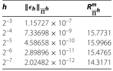
Table 1 Approximation in a rectangle with smooth exact solution
h h
h R
m h 2–3 1.15727×10⁻⁷
2–4 7.33698×10⁻⁹ 15.7731
2–5 4.58658×10⁻¹⁰ 15.9966
2–6 2.89896×10⁻¹¹ 15.4765
2–7 2.02482×10⁻¹² 14.3171
Table 2 Approximation in a rectangle with less smooth exact solution
h hh Rm
h 2–3 1.9285677×10⁻⁴
2–4 1.1998304×10⁻⁵ 16.0737
2–5 7.4809403×10⁻⁷ 16.0385
2–6 4.67808169×10⁻⁸ 15.9915
2–7 2.922653×10⁻⁹ 16.0063
with the boundaryγ. The hexagonal grid (.), denotedh, is assigned to the grid, whereγhdenotes the set of nodes on the boundaryγ.
We consider the problem
u= onh,
u=v(x,y) onγh,
where
v(x,y) =eysinx (.)
is the exact solution in the rectangular domain.
This example is solved using the incomplete LU-decomposition method (see [], Ch. ), and all the calculations are carried out in double precision. As a convergence test, we request the maximum residual error to be –, and as a starting pointv
h= is used. Table gives the values obtained in the maximum norm of the difference between the exact and the approximate solutions, for the values ofh= –k,k= , , , , ,i.e.,
hh=
max
h|v–vh|. The ratiosR
m
h=
v–v–mh
v–v –(m+)h
have also been included, whereO(h) order
of accuracy corresponds to of the valueRm
h.
Example .Less smooth function. We consider the same problem as in Example . with the exact solution
v(x,y) = ln x
+yRez–tan–
y x
Imz, (.)
which is less smooth than (.). The results obtained are consistent with the theoretical results and are summarized in Table .
Table 3 Results for approximation of inner points with the matching operator
S4u 1.56912199976621
Exact 1.56912199014188
| h(P1)| 9.624329×10⁻⁹
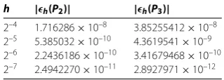
Table 4 Results for approximation of near boundary points with the matching operator
h |h(P2)| |h(P3)|
2–4 1.716286×10⁻⁸ 3.85255412×10⁻⁸
2–5 5.385032×10⁻¹⁰ 4.3619541×10⁻⁹
2–6 2.2436186×10⁻¹⁰ 3.41679468×10⁻¹⁰
2–7 2.4942270×10⁻¹¹ 2.8927971×10⁻¹²
The harmonic function
u(x,y) =excosy (.)
is assumed to be the exact solution. The result in Table is obtained usingh= –and
demonstrates high accuracy of the above constructed matching operator.
The second coordinate considered demonstrates the accuracy of the approximation of near-boundary points. The point chosen isP(., .), whereP∈, and
equa-tion (.) is used for approximaequa-tion. Again, the harmonic funcequa-tion (.) is used as the exact solution. Lastly, a point near one of the corners of the domainP(., .) has
been considered, where the nodes of evaluation emerge outside of the domain from both adjacent sides of the corner. The function
u(x,y) =eycosx
is used as the exact solution. The results obtained are summarized in Table .
Example .Approximation in an L-shaped domain. The final example is solved in an L-shaped domain with an angle singularity at the origin, whereαπ= π/. The domain
is defined by
=
(x,y) : –≤x≤, – √
≤y≤
√
,
where={(x,y) : ≤x≤, –
√
≤y≤}, and is covered by four overlapping rectangles
and a sector. The singular part is defined to be the region
S=
(x,y) : –
≤x≤
, –
√
≤y≤
√
s,
wheres={(x,y) : ≤x≤, – √
≤y≤}, and the nonsingular part is
NS=/S. The
Table 5 The order of convergence in ‘nonsingular’ part
(h,N) hNS Rm
NS (2–4, 40) 9.9742×10⁻⁴ 27.9237
(2–5, 60) 3.57195×10⁻⁵
(2–5, 100) 8.2649×10⁻⁷ 15.3796 (2–6, 100) 5.373923×10⁻⁸
(2–6, 100) 5.373923×10⁻⁸ 15.7215
(2–7, 125) 3.418192×10⁻⁹
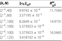
Table 6 The order of convergence in ‘singular’ part
(h,N) hS Rm
S (2–4, 40) 9.9742×10⁻⁴ 11.7569
(2–5, 60) 3.57195×10⁻⁵
(2–5, 100) 8.2649×10⁻⁷ 14.9731
(2–6, 100) 5.373923×10⁻⁸
(2–6, 100) 5.373923×10⁻⁸ 16.5665 (2–7, 125) 3.418192×10⁻⁹
renewed using the matching operator constructed above. Since the boundary functions are harmonic polynomials on the sidesγandγ≡γ, the nodes whose neighbors emerge
outside of the domain from these sides are approximated using the functionu–Q. Finally,
the solution on the singular part is approximated using the integral representation [, ]. The problem considered is
u= onh,
u=v(x,y) onγh,
where
v(x,y) =θ+r/sin
θ
+Rez+Imz,
is the exact solution. Accordingly, the functionQ(x,y) used in the integral representation
is constructed as
Q(x,y) =θ+r cos(θ) +sin(θ)
.
The results in Tables and show the solution for different pairs (h,N), whereN is the number of quadrature nodes,his the mesh size of the hexagonal grid.
6 Conclusions
grid functions. It is applied to construct a fourth order accurate interpolating function, on the closed rectangle, for the numerical solution of Laplace’s equation on the hexagonal grids. Further, the matching operator and the hexagonal grid approximation in a rectangle are used to obtain and justify the Block-Grid method in solving the Dirichlet problem for Laplace’s equation on staircase polygons.
Numerical examples have been provided as an illustration of the theoretical results men-tioned above.
The matching operator constructed can be applied to many other forms of domain de-composition or combined methods. It will also be an interesting study to extend the ap-proximation of the methods to using mixed or Neumann boundary conditions.
Competing interests
The authors declare that they have no competing interests.
Authors’ contributions
All authors contributed equally to the writing of this paper. All authors read and approved the final manuscript.
Received: 28 November 2013 Accepted: 9 March 2014 Published:28 Mar 2014
References
1. Volkov, EA: Method of composite meshes for finite and infinite domain with a piecewise-smooth boundary. Tr. Mat. Inst. Steklova96, 117-148 (1968)
2. Volkov, EA: On the method of composite meshes for Laplace’s equation on polygons. Tr. Mat. Inst. Steklova140, 68-102 (1976)
3. Dosiyev, AA: A fourth order accurate composite grids method for solving Laplace’s boundary value problems with singularities. Comput. Math. Math. Phys.42(6), 832-849 (2002)
4. Dosiyev, AA, Buranay, SC: A fourth order accurate difference-analytical method for solving Laplace’s boundary value problem with singularities. In: Tas, K, Machado, JAT, Baleanu, D (eds.) Mathematical Methods in Engineers, pp. 167-176. Springer, Berlin (2007)
5. Dosiyev, AA, Buranay, SC: A fourth-order block-grid method for solving Laplace’s equation on a staircase polygon with boundary functions inCk,λ. Abstr. Appl. Anal.2013, Article ID 864865 (2013). doi:10.1155/2013/864865 6. Dosiyev, AA, Buranay, SC, Subasi, D: The highly accurate block-grid method in solving Laplace’s equation for
nonanalytic boundary condition with corner singularity. Comput. Math. Appl.64, 612-632 (2012)
7. Dosiyev, AA: A block-grid method for increasing accuracy in the solution of the Laplace equation on polygons. Russ. Acad. Sci. Dokl. Math.45(2), 396-399 (1992)
8. Dosiyev, AA: A block-grid method of increased accuracy for solving Dirichlet’s problem for Laplace’s equation on polygons. Comput. Math. Math. Phys.34(5), 591-604 (1994)
9. Dosiyev, AA: The high accurate block-grid method for solving Laplace’s boundary value problem with singularities. SIAM J. Numer. Anal.42(1), 153-178 (2004)
10. Volkov, EA, Dosiyev, AA: A high accurate composite grid method for solving Laplace’s boundary value problems with singularities. Russ. J. Numer. Anal. Math. Model.22(3), 291-307 (2007)
11. Samarskii, AA: The Theory of Difference Schemes. Dekker, New York (2001)
12. Niˇckovic, S, Gavrilov, MB, Tošic, IA: Geostrophic adjustment on hexagonal grids. Mon. Weather Rev.130(3), 668-683 (2002)
13. Majewski, D, Liermann, D, Prohl, P, Ritter, B, Buchhold, M, Hanisch, T, Paul, G, Wergen, W, Baumgardner, J: The operational global icosahedral-hexagonal gridpoint model GME: description and high-resolution tests. Mon. Weather Rev.130(2), 319-338 (2002)
14. Sadourny, R, Morel, P: A finite-difference approximation of the primitive equations for a hexagonal grid on a plane. Mon. Weather Rev.97(6), 439-445 (1969)
15. Volkov, EA: On differentiability properties of solutions of boundary value problems for the Laplace and Poisson equations on a rectangle. Proc. Steklov Inst. Math.77, 101-126 (1965)
16. Kantorovich, LV, Krylov, VI: Approximate Methods of Higher Analysis. Noordhoff, Groningen (1958)
17. Volkov, EA: Block Method for Solving the Laplace Equation and Constructing Conformal Mappings. CRC Press, Boca Raton (1994)
18. Volkov, EA: An exponentially converging method for solving Laplace’s equation on polygons. Math. USSR Sb.37(3), 295-325 (1980)
19. Smith, GD: Numerical Solution of Partial Differential Equations: Finite Difference Methods. Oxford University Press, Oxford (1985)
10.1186/1687-2770-2014-73