Optimizing Virtual Backup Allocation for Middleboxes
Yossi Kanizo
Computer Science
Tel-Hai College
[email protected]
Ori Rottenstreich
Computer Science
Princeton University
[email protected]
Itai Segall
Bell Labs
Nokia
[email protected]
Jose Yallouz
Electrical Engineering
Technion
[email protected]
Abstract—In enterprise networks, network functions such as address translation, firewall and deep packet inspection are often implemented in middleboxes. Those can suffer from temporary unavailability due to misconfiguration or software and hardware malfunction. Traditionally, middlebox survivability is achieved by an expensive active-standby deployment where each middlebox has a backup instance, which is activated in case of a failure. Network Function Virtualization (NFV) is a novel networking paradigm allowing flexible, scalable and inexpensive implementation of network services. In this work we suggest a novel approach for planning and deploying backup schemes for network functions that guarantee high levels of survivability with significant reduction in resource consumption. In the suggested backup scheme we take advantage of the flexibility and resource-sharing abilities of the NFV paradigm in order to maintain only a few backup servers, where each can serve one of multiple functions when corresponding middleboxes are unavailable. We describe different goals that network designers can take into account when determining which functions to implement in each of the backup servers. We rely on a graph theoretical model to find properties of efficient assignments and to develop algorithms that can find them. Extensive experiments show, for example, that under realistic function failure probabilities, and reasonable capacity limitations, one can obtain 99.9% survival probability with half the number of servers, compared to standard techniques.
I. INTRODUCTION
Enterprise networks often rely on middleboxes to support a variety of network services such as Network Address Translation (NAT), load balancing, traffic shaping, firewall and Deep Packet Inspection (DPI). Typically, a middlebox is dedicated to implement solely a single function without a common standardization among different vendors, raising the complexity and cost of middlebox management.
Middlebox failures might occur frequently, inducing great degra-dation of service performance and reliability [1]. Failures might occur due to several reasons, such as connectivity errors (e.g., link flaps, device unreachability, port errors), hardware faults (memory errors, defective chassis), misconfiguration (wrong rule insertion, configuration conflicts), software faults (reboot, OS errors) or ex-cessive resource utilization. Temporary inability to support network functions can lead to packet drops, reset of connections, redundant packet delays, and in some cases even to security issues. A common approach for achieving middlebox reliability is through redundancy, where an additional instance of each middlebox operates as a backup upon a failure of the first [2], [3]. This approach is often referred to as active-standby deployment, where one (the “active”) instance handles all the traffic, while a second (the “standby”) instance is mostly inactive, until a failure occurs. Once a failure is identified, all traffic is diverted to the standby instance, which has to immediately handle the functionality of the active one. While
this approach enables simple dealing with a failure in each of the active middleboxes, it is often too restrictive and demands excessive redundancy in practice, especially since the frequency of failures can vary for different middleboxes, in addition to that usually not all the middleboxes encounter problems concurrently. Therefore, a milder and more flexible survivability approach is called for, which would relax the rigid requirement of an entire dedicated copy per active function.
Network Function Virtualization (NFV) [4] is a recent popular paradigm by which network functions are executed on commodity servers managed by a centralized software defined mechanism. Such virtual middleboxes are often also referred to as Virtual Network Functions (VNFs). By its elastic nature, NFV can consid-erably reduce operating expenses. Specifically, we show how the flexibility of NFV can be utilized for planning of efficient backup schemes for running functions, while better utilizing resources to support recovery from failures.
A significant cost reduction can be achieved through sharing of resources, servers in the context of NFV, among the standby instances of the different functions. Our suggested backup solution consists of multiple servers, with a typical number smaller than the number of existing middleboxes. In order to introduce the cost reduction we take advantage of the low resource utilization of the backup instances. A server is therefore assumed to have the capability to backup several functions, namely some specific selected subset of functions. As soon as a failure occurs, a server is turned into an active instance of the function of the failed middlebox, discarding the other backup capabilities of that server. Note that as a standby machine, the server can backup multiple functions. Once becoming active, only one of those functions can be served by this server. We show that while causing a very low penalty in terms of survivability, our suggested backup scheme enables a significant reduction in the amount of required resources in comparison with the conventional active-standby approach.
server%S1%
LB%
%
DPI%
FW%
NAT%
% network%%
func:ons% backup%servers%virtualized%%
LB# NAT# IDS#
1%%%%%%%%%%%%%2%%%%%%%%%c=3%%%
IDS%
server%S2%
LB# DPI# IDS#
1%%%%%%%%%%%%%2%%%%%%%%%c=3%%%
server%S3%
LB# FW# NAT#
1%%%%%%%%%%%%%2%%%%%%%%%c=3%%%
(a) Architecture ofk= 5
func-tions andn= 3servers
LB
DPI
FW
NAT
IDS
S1
S2
S3
(b) Bipartite graph represen-tation. Left: network func-tions, right: Servers.
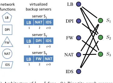
Fig. 1. (a) Illustration of architecture for middlebox survivability. A server can be used to backup one ofc= 3predetermined functions. To do so, the server must be frequently synchronized about the state of each of the functions it can backup. (b) Bipartite graph representation of the assignment of functions to servers. The degree of a server node is restricted to the capacityc.
staying in standby to replace any one of them, is limited and is expected to remain relatively low.
Network management under this aggregated standby mode should consider an important decision, namely the selection of the set of functions to be backed up in each of the servers. We demonstrate how this assignment affects the backup capabilities, and determines the possible combination of middlebox failures that can be resolved. Recall that in the case of two functions with faulty middleboxes, a single server that supports both functions cannot run more than one of them. In this work, we focus on aiming to optimize the backup scheme for maximum survivability under a given resource allowance. We detail several metrics describing goals that a network manager should take into account to achieve better survivability utilizing the constrained amount of resources.
Fig. 1(a) illustrates such a survivability architecture with five functions and three servers for backup. Each of the servers keeps the updated information required to recover three of the functions. In this example, for the load balancing function (LB), for instance, there is a backup in all the three servers and accordingly it can be recovered by any of them while for the deep packet inspection function (DPI) there is a backup in only one of the servers. Of course, information regarding the failure models and in particular their failure probabilities can be considered in the assignment of functions to servers to achieve higher survivability.
We investigate how to provide the best survivable solution supported by this approach of shared resources. To that end, we formalize two optimization problems describing possible goals that a network manager would often like to achieve in Section II. These problems consider the probability of full recovery from failures, as well as the expected number of functions that are available following a set of failures and the recovery process. In Section III and Section IV we establish fundamental properties of the problems while relying on tools from graph theory. We describe characteristics of optimal solutions, show bounds on the performance of optimal solutions, and demonstrate that both problems are NP-hard. Then, based on this analysis, we provide
in Section V several algorithms to find efficient assignments. In Section VI we further discuss our findings about the problems such as providing guarantees on the performance of the solutions. In Section VII we demonstrate the advantages of our solutions through comprehensive simulations. Related work can be found in Section VIII. Finally, Section IX summarizes our results and discusses directions for future work.
II. MODEL ANDPROBLEMDEFINITION
We analyze this backup scheme through a graph framework. We denote the set of all functions by F and their number by k =
|F| such that F ={1, . . . , k}. Likewise, let n be the number of
servers and let c be the constrained capacity of a server, i.e., the
maximal number of functions it can support. We refer to the set of servers by S satisfying |S| = n. We view an instance of the model as a bipartite graphFSSwithk+nnodes. The assignment of functions to servers determines its edges. An edge between a server to a function illustrates the support of the function by the server. Fig. 1(b) shows the bipartite graph that corresponds to the assignment from Fig. 1(a). The capacity of the server limits its degree to at mostcwhile the degree of a function equals the number
of servers implementing it with a value in [0, n].
A functioni2F is associated with a failure probabilitypi. We
assume that these probabilities are mutually independent as well as that the servers are always operational, i.e. do not encounter failures. These probabilities determine the possibility for every set of functions,H ✓F, to appear as the set of faulty functions.
Upon a failure in a subset of the network functions H, we
are often interested in the induced graph of the set of faulty functionsH, their outgoing edges and the connected set of servers.
Operational functions do not have to be recovered. A matchingM
describes the possibility to recover|M|of the functions inH, such
that a function can be recovered by its matched server. A matching of size|M|=|H| would enable recovering all faulty functions.
While managing the network, various goals considering surviv-ability can be taken into account. Ideally, we would like to verify that all functions have an operational instance. This would enable to successfully serve all traffic, regardless of the network functions that a specific flow requires to apply. In interesting scenarios the number of backup servers is smaller than that of the functions and it is thus impossible to guarantee that all functions are operational or can be recovered. To that end, we would like to maximize the probability of the scenario that all functions have an operational instance, as expressed in the first optimization problem studied in this work.
Problem 1. Given are a set of functions F with function failure probabilities, a number of servers n, each with capacity c. The aim is to find an assignment that maximizes the probability for a recovery of all faulty functions. In such a recovery, each server is matched to at most one failed function, and each failed function is matched to one server.
We denote byPOP T the optimal, maximal possible probability.
[image:2.612.71.258.53.191.2]scheme – an assignment of functions to servers, calculating the probability for full recovery for this assignment can be a difficult task that requires considering a large number of combinations of faulty functions.
Sometimes there exists a benefit from a partial recovery of the faulty functions. Accordingly, the next problem tries to maximize the number of available functions, i.e. the number of functions with operating middleboxes in addition to the maximal size set that can be recovered.
Problem 2. Given are a set of functions F with function failure probabilities, a number of servers n, each with capacity c. The aim is to find an assignment maximizing the expected number of operating functions.
This problem is equivalent to trying to maximize the expected number of functions that are recovered. The two metrics differ by a constant, equal to the expected number of operating functions without the recovery. We denote by EOP T the optimal, maximal
expected number of operating functions.
In both problems, finding a recovery is performed for a given status of the middleboxes, i.e. indication which of them is not operating. In other words, we assume that all functions fail at once. When the assignment of functions to servers is known, as well as the set of failed functions, a recovery of a maximal number of failed functions, expressed by a matching in the induced graph, can be easily found (in polynomial time) using algorithms for maximum matching in bipartite graphs (e.g., [7], [8]).
Our model has several simplifying assumptions. First, it assumes that all functions require the same capacity when being backed up by a server. In addition, we don’t consider a potential correlation between failures of different functions. The model also assumes that the physical location of a function implementation does not affect the performance. We leave model generalizations for future work.
III. PROBLEM1: FULLRECOVERYPROBABILITY In this section we address Problem 1. We would like to find an assignment that maximizes the probability that all functions are operational or can be recovered. While the problem is rather easy when each server has a capacity of 1, we show that for a larger capacity the general problem is NP-hard.
For the set of k functionsF ={1, . . . , k} let {p1, p2, . . . , pk}
be the respective function failure probabilities. W.l.o.g. assume functions have non-zero failure probabilities (a function that never fails does not require a backup) that are ordered in a non-decreasing order p1 p2 · · · pk, i.e., the earlier functions are more
reliable. Denote by p the product of those k probabilities. The
set of n servers is denoted by S = {S1, S2, . . . , Sn}, each with
capacityc.
A simple observation is that it is impossible to guarantee a recovery of any combination of failed functions with less than
n = k servers. Due to the independence of functions, they can
all fail together even if this scenario has a very small probability. It is also easy to guarantee that with at leastkservers by dedicating
a server to each function.
Corollary 1. The optimal full recovery probability satisfies POP T <1 when the number of servers isn < k and POP T = 1 whenn k.
We now turn to discuss the simple case ofc= 1, where a server
cannot backup more than one function.
A. Simple Case:c= 1
Theorem 2. In case c = 1, the optimal assignment of functions to servers is by assigning the nservers with the n functions with top failure probability, each server to a different function. Con-sequently, the optimal full recovery probability satisfies POP T =
Qk n
i=1 (1 pi), i.e. the probability that all firstk nfunctions do not fail.
Proof. Once a function is recovered by some server, all other servers that are assigned to this function are useless (each server is assigned with only one function in our case). Therefore, all n
servers should be assigned to distinct functions. Then, the first part of the theorem easily follows. Finally, full recovery is achieved if and only if none of the otherk nfunctions fail, which yields the
second part of the theorem.
B. Problem Hardness
We now focus on the case wherec= 2. This case is much more complicated to analyze and to solve. In fact, a capacity of c= 2
suffices to show that the problem is NP-hard.
Our proof for the NP-hardness of this problem provides an intuition on how it can be solved approximately and inspired us in the design of the approach we take to tackle this problem later. The basic idea is to focus on the connected components of the underlying bipartite graph. In each connected component, nodes represent either servers or functions. The following two properties follow from [9]:
Property 3. In case c = 2, each connected component with t servers has at most t+ 1 functions.
Property 4. In case c= 2, let C be a connected component with t servers and q t+ 1 functions. Then for each subset of size min{t, q} of functions, there is a matching containing all of the functions.
To see the intuition behind these properties note that we can add to a connected component a server, by assigning one of its c= 2
functions to one that already belongs to the component. Therefore this addition adds a single additional server and an additional single function. Its connectivity ensures finding such a matching.
The next theorem is easily followed:
Theorem 5. In casec= 2, and n < k, i.e., the number of servers is lower than the number of functions, each connected component in an optimal solution contains a number of functions that is larger by one than the number of servers.
Proof. Consider an optimal solution. Sincen < k there is at least
one component with a number of servers smaller than the function number by exactly one. Difference cannot be larger by Property 3. We denote one such component byC1. If the current theorem does
1
2
3
4
5
S1
S2
S3
S4
(a) non-optimal assignment I, 2 connected components
1
2
3
4
5
S1
S2
S3
S4
[image:4.612.67.264.51.175.2](b) optimal assignment II, a sin-gle connected component
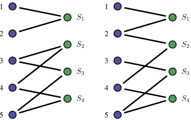
Fig. 2. Illustration of the structure of the bipartite graph in an optimal assignment forc= 2(Theorem 5). Left: network functions. Right: Servers. Survival probability is improved when reducing the number of connected components as in a transition from (a) to (b) with the change of a one edge.
tfunctions. We show that the two components can then be merged
to increase the probability for recovery of all failing functions, in contradiction to the optimality of the solution.
By Property 4 all functions inC1can be recovered as long as not all of them fail together. We say then that the survival probability of the component is 1 PC1 = 1
Q
i2FC1pi. Similarly, by the
same property, we can always recover any set of failing functions fromC2, even if they all fail. Thus all functions inC1, C2 can be recovered with probability 1 PC1.
For an arbitrary spanning tree of C2, consider an edge of the
connected component that is not included in the tree. Since there arec·t= 2tedges, there must be such an edge not included in the
at mostt+q 12t 1edges in the spanning tree. Omitting this
edge does not eliminate the connectivity of C2. We can therefore
merge the two components C1, C2 by connecting one such edge to an arbitrary function in C1, without changing the server it is connected to. Then, we obtain one connected componentCinstead of the two C1, C2, with t0 servers and q0 t0 + 1 functions.
Failures within its functions can be fully recovered with probability
1 PC = 1 Qi2FCpi= 1
Q
i2FC1 S
FC2pi>1
Q
i2FC1pi,
i.e., larger than before the merge operation. Recovery probabilities for the other connected components are not affected by the change. Such a change is illustrated in Fig. 2 where in (a) there are two connected components C1 with functions{1,2} and a single server andC2 with functions{3,4,5}and three servers. In (b), by changing a single edge betweenS2 to function2 instead of3, the number of connected components is reduced to one, improving the survival probability.
By Theorem 5, the total number of functions equals the number of servers plus the number of connected components. This enables us to express the number of connected components in an optimal solution.
Theorem 6. In casec = 2, andn < k, the number of connected components in an optimal solution is k n. This is the minimal possible number of components under these assumptions.
We now turn to compute the survival probability of a connected component.
Theorem 7. In case c = 2, and n < k. Let C be a connected component in an optimal assignment, and let {f1, . . . , fq} be the set of all function indices inC. Then the survival probability of the connected component is given by1 Qqi=1pfi.
Proof. By Theorem 5 we get that the number of functions in
C is t+ 1 while the number of servers is t, for some t 2 N. Therefore, for each subset of functions of sizetthere is a matching in C (Property 4). Consequentially, the only case where not all functions can be recovered is the case where all of them fail. This happens with probabilityQq
i=1pfi. The survival probability follows
by taking the complement.
Next, one may compute the overall survival probability, which is given by the product of the survival probability of all connected components. This follows immediately from the independence of function failure probabilities.
Theorem 8. In case c = 2, and n < k, the overall survival probability is given by the product of all connected component survival probabilities.
We begin to have a clear picture on how an optimal assignment looks like, as an intuition on how to split the connected components in the graph. Informally, we would want the connected components’ survival probabilities to be balanced. We start with the special case where an optimal solution has two connected components.
Intuitively, there is a dependency between functions within the same connected component such that it might be impossible to recover one upon some scenario of others. Consider two functions
i, j with failure probabilitiespi> pj. Assume their backup should
be selected from two available server slots, each translated to adding the function to one of two connected components C1, C2 with current failure probabilitiesPC1> PC2. Since functionifails more
often, we wish to prioritize it. Thus it would be better to place it in the connected component with more reliable existing functions, i.e. in C2. The other function, j, which encounters failures less frequently, will be placed in C1 with existing functions that are more failure-prone. This addition will contribute to the balancing of the two failure probabilities of the two connected components. Theorem 9. In casec= 2, andk=n+2, the optimal solution has
exactlytwo connected components. Among all possible assignments such that the bipartite graph has two connected components C1 andC2with respective connected component survival probabilities 1 PC1 and 1 PC2, the optimal assignment is the one for which max{PC1,PC2}
min{PC1,PC2}
is minimized. In particular, if PC1 = PC2 the assignment is optimal.
Proof. First, since k = n+ 2, by Theorem 6 the number of
connected components is k n= 2. LetA be an assignment that
results in two connected components C1 and C2 with respective
connected component survival probabilities1 PC1 and1 PC2.
Also, let r = max{PC1,PC2}
min{PC1,PC2}. Assume that there exists an
assign-ment A0 with the corresponding C0
r0 = max{PC01,P 0
C2} minnP0
C1,P 0
C2
o, such that r0 < r. Since there exist exactly
two connected components in each assignment, a function not included in one component must be included in the second and
C1\C0
1=C20 \C2 andC2\C20 =C10 \C1.
We will show that the survival probability of the assignment A0
is larger than the corresponding probability of the assignment A,
i.e. that(1 PC01)(1 P 0
C2)>(1 PC1)(1 PC2).
To show this, we assume w.l.o.g. that PC1 PC2 and PC01 P0
C2. This implies that PC1 PC2 >
PC01 P0
C2.
We define ↵ = PC1\C01 and = PC2\C20. In words, ↵ is the
product of probabilities of the functions that are assigned to the first connected component in both solutions, and similarly for the second component.
We further define a = PC1\C10 = PC20\C2 and b = PC2\C20 = PC0
1\C1. That is, a is the product of probabilities of the functions
that are assigned to the first connected component in the solution
A, but not to the first in A0. Note that P
C1 = a·↵. Therefore, PC0
2 =a· . Symmetrically,PC2 =b· andPC10 =b·↵. PC1
PC2 > P
0 C1 P0
C2
) a↵b > b↵
a )a
2> b2
)a > b
PC01 P 0
C2)b·↵ a· > b· )↵>
By combining both of the above,a(↵ )> b(↵ )
)a↵+b > b↵+a
)PC1+PC2 > PC10 +PC20 )1 +p PC0
1 PC20 >1 +p PC1 PC2 )(1 PC01)(1 P
0
C2)>(1 PC1)(1 PC2).
We are now ready to show that the general problem is NP-hard. The proof is based on reducing the number partitioning problem [10] to our problem. In this problem, the goal is to divide a multiset of positive integers into two disjoint subsets while minimizing the absolute value of the difference of the subset sums. Theorem 10. Finding an optimal assignment for Problem 1 is NP-hard (even forc= 2).
Proof. Let the positive integer multiset X denote an instance of the number partitioning problem, with X ={x1, x2, . . . , xt}. We
construct in polynomial time an instance of the assignment problem, so that by finding the optimal assignment one can deduce the optimal number partitioning, i.e., a partition of the multisetX into
two (disjoint) subsetsX1 andX2such that the difference between
the sum of the integers in the subsets is minimized.
Given the multiset X, we construct k = t functions (left-side vertices), where a failure probability of e xi is assigned to the
function i 2 F. Last, we choose to use n = k 2 servers with capacityc= 2.
By Theorem 9, the optimal assignment has two connected com-ponents, and among all possible assignments with a corresponding bipartite graph of two connected components, the optimal assign-ment is the one that minimizes max{PC1,PC2}
min{PC1,PC2}
. Assume w.l.o.g.
thatPC1 PC2. Thus, the optimal assignment minimizes PC1 PC2. By
taking logon this expression, we get that it also minimizes
log
✓P
C1 PC2
◆
= log (PC1) log (PC2).
LetFC1 be the set of all function indices inC1. By Theorem 7,
log (PC1) = log
0 @ Y
i2FC1 pi
1 A= X
i2FC1
log (pi) =
X
i2FC1 xi.
LetFC2 be the set of all functions indices inC2. Similarly,
log
✓P
C1 PC2
◆
= X
i2FC2 xi
X
i2FC1 xi.
Since we assumed that PC1 PC2, the above expression is
non-negative, that is, the first summation is at least as big as the second one.
We get that, among all possible partitions into two subsets, the optimal assignment minimizes the difference between the sum of subsets, i.e., it solves the number partitioning problem.
C. Bounds
In this section we describe an upper bound on the value of the optimal full recovery probabilityPOP T for the case ofc= 2.
We start with the following simple lemma.
Lemma 1. Foru1, u2, u3, u4satisfying0< u1< u2u3< u4< 1 andu2·u3=u1·u4. Then,u2+u3< u1+u4.
Proof. By the equality u2·u3 = u1·u4 we deduce u2·u3 = (u1+ (u2 u1))·(u4 (u4 u3)) =u1·u4 u1·(u4 u3) + (u2 u1)·u4 (u2 u1)·(u4 u3)and accordingly(u4 u3)· (u1+ (u2 u1)) = (u2 u1)·u4. Since (u1+ (u2 u1))< u4
(and all four parts in the two products are positive) then necessarily
(u4 u3)>(u2 u1)and the inequality follows. We suggest the following upper bound.
Theorem 11. In case c= 2, the optimal full recovery probability satisfies POP T
⇣
1 pk1n
⌘k n
, where p = Qki=1pi is the product of all function failure probabilities.
Proof. We focus on some optimal solution. By Theorem 6, the number of connected components in an optimal solution is k n. Let, PC1, PC2, . . . , PCk n be the connected component failure
probabilities. By Theorem 8, the full recovery probability is then given by Qk n
i=1 (1 PCi). To maximize the full recovery
proba-bility one needs to take into account the fact that the connected components failure probabilities are a result of the product of the function failure probabilities within each connected component. To show the upper bound we relax this constraint and only maximize the full recovery probability subject to the constraint that Qk n
i=1 PCi =
Qk
i=1pi = p. We show that this probability
is achieved when every component has a survival probability of
1 pk1n. Starting from an arbitrary solution we present a sequence
of changes that improve the survival probability until we obtain the bound. If not all components have a failure probability ofpk1n, we
can find two components indexedi, jsuch thatPCi < p 1 k n < P
We denote u1 = PCi, u4 = PCj and u2 as one of the values pk1n, u1·u4·p k1n andu3 as the other value such thatu2u3.
They satisfy u1·u4 = u2·u3 and u1 < u2 u3 < u4 since u1, u42(0,1]. We show that by setting the failure probabilities of the two components to beu2andu3, the survival probability of the solution is improved. To do so we compare(1 u2)·(1 u3)with
(1 u1)·(1 u4) since other connected connected components are not affected by the change. We haveu2·u3 =u1·u4 and by Lemma 1u2+u3< u1+u4and accordingly(1 u2)·(1 u3) = 1 u2 u3+u2·u3>1 u1 u4+u1·u4= (1 u1)·(1 u4).
Finally, after no such additional pairs can be found, we obtain a survival probability of ⇣1 pk1n
⌘k n
and the probability of the initial legal solution cannot be larger.
IV. PROBLEM2:EXPECTED NUMBER OF RECOVERED FUNCTIONS
Sometimes there can be a benefit from any available function that is running. In this section we study Problem 2, where we try to maximize the number of such functions, i.e. the functions with an operating middlebox together with the set of functions that can be recovered. We recall that we refer to the optimal (maximal) value of the expected number of such functions asEOP T.
We can easily observe thatEOP T increases for larger number of
serversnand thatEOP T =konly forn k(assumingpi>0), i.e.
when the number of servers equals at least the number of functions. A given assignment determines the connected components in the bipartite graph. Then, by the linearity of expectation the expected number of operating functions is given by the sum of their number in each connected component.
Problem 1 and Problem 2 are similar since in both problems it is more important to be able to recover a function that fails more frequently, i.e. with a larger failure probability. The difference comes from the fact that the first problem does not benefit from a partial recovery of the non-operating middleboxes. While we show that the problems coincide for some families of inputs we demonstrate that they differ in the general case.
A. Similarity of Problem 2 to Problem 1 and its NP-Hardness
We now show that the two problems collide for the casec= 2
andk=n+2and their optimal solutions then coincide. This allows
us to deduce that Problem 2 is also NP-hard.
We again rely on Property 3 and Property 4 that hold for general bipartite graphs (withc= 2). Since in a connected component oft
servers andq=t+1functions, all failed functions can be recovered as long as not all theq functions fail we deduce the following. Theorem 12. In a connected component C of t servers and q= t+ 1functionsFC, the expected number of operating functions in this component isEC=q Qi2FCpi.
We show that Theorem 5 holds also for this problem.
Theorem 13. In casec= 2, andn < k, i.e., the number of servers is lower than the number of functions, each connected component in an optimal solution to Problem 2 contains a number of functions that is larger by one than the number of servers.
Proof. The proof is similar to the proof of Theorem 5. If the theorem does not hold, there exist two componentsC1, C2such that
by merging them we can increase their contribution to the expected number of available functions from|FC1|+|FC2|
Q
i2FC1pi to
|FC1|+|FC2|
Q
i2FC1 S
FC2pi.
By Theorem 13, we get that also for Problem 2, if c = 2 and
n < kin an optimal solution the number of connected components isk n.
We now show that forc= 2, andk=n+2, the optimal solutions of Problem 1 and Problem 2 coincide.
Theorem 14. In casec= 2, andk=n+ 2, the solution is exactly the same as in the maximum recovery probability problem. Proof. As before, since k = n+ 2, the number of connected
components isk n= 2. We denote the two connected components
byC1andC2 with function index setsFC1 andFC2, respectively.
Also, let their respective expected number of running functions be |FC1|
Q
i2FC1pi and |FC2|
Q
i2FC2pi. By Theorem 12, the
overall expected number of running functions is given by:
|FC1|
Y
i2FC1
pi+|FC2|
Y
i2FC2 pi =k
Y
i2FC1 pi
Y
i2FC2 pi.
In Problem 1 one minimizes the expression
0
@1 Y i2FC1
pi
1 A·
0
@1 Y i2FC2
pi
1 A=
1 Y
i2FC1 pi
Y
i2FC2 pi+
Y
i2FC1 pi·
Y
i2FC2 pi.
Note that the last product of products is actually constant, regardless of the partition into two connected components.
By disregarding constants, we get that a solution that performs better than another in one problem has an improved performance also for the second problem. Therefore, optimality is achieved by the same solution.
Finally, we deduce that Problem 2 is NP-hard. The proof is based on the fact that for c = 2, and k = n+ 2 the optimal solutions of the two problems coincide and in Theorem 10 Problem 1 was shown to be NP-hard for this case.
Theorem 15. Finding an optimal assignment for Problem 2 is NP-hard (even forc= 2).
B. Bounds
We present an upper bound on the expected number of available functions. For the sake of brevity, we omit the proof of the next theorem, which follows the lines of the proof of Theorem 11. Theorem 16. In case c = 2, the optimal expected number of available functions satisfies EOP T k (k n)·p
1
k n, where
1,e 2.2
2,e 2.1
3,e 2
4,e 1.2
5,e 1.1
6,e 1
S1
S2
S3
(a) optimal assignment I
1,✏
2,e 2.1
3,e 2
4,e 1.2
5,e 1.1
6,e 1
S1
S2
S3
(b) assignment II, optimal for small✏
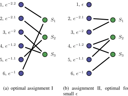
Fig. 3. Illustration of the distinction between Problem 1 and Problem 2 (Sec-tion IV-C). Left: network func(Sec-tions. Right: Servers. The failure probability appears for each function. When changing the failure probability of the first functionp1
frome 2.2to a small✏>0, the optimal assignments for each of the two problems
changes from assignment I (in (a)) to assignment II (in (b)).
C. Between the two optimization problems
Based on the similarity between Problem 1 and Problem 2 as we detailed, one might wonder whether the two problems are identical. The next example demonstrates that the two problems differ from each other by showing how to find an instance where optimal assignments for the two problems vary. Let k = 6
and n = 3, c = 2, and first consider the failure probabilities be p1, . . . , p6 = e 2.2, e 2.1, e 2, e 1.2, e 1.1, e 1. An optimal
assignment to Problem 1 (assignment I) is with connected com-ponents C1 = {1,6}, C2 = {2,5}, C3 = {3,4} (achieved for servers implementing functions {1,6},{2,5},{3,4}). It achieves
full recovery probability ofPOP T = (1 p1·p6)·(1 p2·p5)·(1 p3· p4) = (1 e 3.2)3= (1 p13)3forp=Qk
i=1pi. The solution must
be optimal since it achieves the upper bound from Theorem 11. This is also an optimal solution for Problem 2 achieving an expected number of k p1 ·p6 p2 ·p5 p3 ·p4 = 6 3·e 3.2 = k (k n)·pk1n available functions as in the upper bound from
Theorem 16. If we set p1 = ✏ (i.e., arbitrarily small), for both problems, there is no need to backup the first function and for both problems an optimal assignment (assignment II) has the connected components C0
1 ={1}, C20 ={2,3}, C30 ={4,5,6} (achieved for
instance for servers implementing functions{2,3},{4,5},{4,6}). Moreover, for p1 2 [✏, e 2.2] the transition value of p1 between
the two optimal solutions is different for the two problems. For Problem 1 we compare (1 p1·p6)(1 p2·p5)(1 p3·p4) =
(1 p1)(1 p2·p3)(1 p4·p5·p6) and get a transition point
of p2·p3 p2·p5 p3·p4+p4·p5·p6+p2·p3·p4·p5 p2·p3·p4·p5·p6
p6+p2·p3 p2·p5·p6 p3·p4·p6+p4·p5·p6 1 ⇡0.044390.
For Problem 2 we compare 6 p1· p6 p2 ·p5 p3· p4 = 6 p1 p2 · p3 p4 · p5 ·p6 and get a transition point of
p2·p3 p2·p5 p3·p4+p4·p5·p6
p6 1 ⇡0.044404. Ifp1 is set to be between
the two transition points, we have different optimal solutions for the two problems. The two assignments are illustrated in Fig. 3.
V. SOLUTIONS
We suggest various approaches to tackle the two problems. The solutions apply to both problems due to their similarity.
A. Simple Random Assignment (SRA)
The first approach is mainly used as a reference to the algorithms described in Section V-B and Section V-C.
In the SRA algorithm, we pick, randomly and independently, for each server c different functions that it backups, where the probability to choose any function is proportional to the specific function failure probability. The exact steps are described below:
• Compute the proportional probability vector defined by
{p1, p2, . . . , pk}/Ppi. • For each serverSj, j2[1, n]:
– Letvj=v.
– For each of the c backup slots: Randomly and
indepen-dently pick a function using the distribution defined invj.
Updatevj by removing the function that was picked and
normalize back to a sum of 1.
B. Constrained Random Assignment (CRA)
Based on the intuitions obtained above we perform a slight modification to the SRA algorithm where the effect of the value of the failure probability of a function on the number of instances is moderate.
The basic idea is to decide in advance how many backups each function has, and then distribute the backups to the servers. The number of backups should be as even as possible, with a maximal difference of one. The exact steps are described below:
• Decide on the number of backups bi for function i 2[1, k].
Start with bn· c/kc backups for each one. Add an extra
backup to the functions with the top (n·c) modk failure
probabilities.
• For each serverSj, j2[1, n], select randomlycamong then·c
instances, avoiding multiple selections of the same function by the same server.
C. Balanced Assignment (BA)
The following approach is also based upon the intuitions from the analysis. It consists of three phases:
• Decide on the number of connected components. As was
shown, a crucial aspect in the effectiveness of a backup scheme is the partitioning of the corresponding bipartite graph into connected components. Therefore, in the first phase we choose the number of such components to partition the graph into.
• Partition the functions into the connected components. As
discussed, the aim is to partition the functions such that the product of failure probabilities for functions in each component is balanced.
• Construct the actual backup scheme, by assigning functions to
servers.
[image:7.612.64.271.60.216.2]1) Deciding on the number of connected components: General-izing on Theorem 6, we wish to minimize the number of connected components. Therefore, given k functions, and n servers with
capacity c, we choose to construct t = max(1, k (c 1)·n)
connected components.
2) Partitioning the functions into the connected components:
Generalizing on Theorem 9, the aim of the partitioning is to balance as much as possible the product of failure probabilities of functions in each partition. We choose a greedy approach to this problem. First, functions are sorted in non-decreasing order of their failure probability. Then, each function is assigned to the partition with the largest product of failure probabilities so far.
In order to allow a mapping of the functions in each partition to servers, that is consistent with the choice of t above, we require
the size of each partition to be(c 1)·w+ 1for some integerw.
If in the result of the greedy algorithm this is not the case, we shift functions between partitions. In order for this to affect the balance between the partitions the least, we choose to shift the functions with the highest failure probability.
3) Constructing connected components from the partitions: Each set of functions partitioned together in the previous step should now get a set of servers, and mapping between the functions and servers, such that a connected component is formed in the corresponding bipartite graph. Clearly, the construction of each component is independent of the other components, so we focus on a single given component.
Assuming the connected component consists off functions, let z = fc 11 be the minimal number of servers required in order
to construct a connected component for these functions. We re-partition thef functions intoz partitions, under the constraint that
no partition contains more thancfunctions, using the same greedy heuristics as before. Each such partition is then mapped to a single server. For each remaining backup slots, i.e. for each server that received less than c functions, we connect the functions with the maximal failure probability from the previous partitions until c
functions are backed up. This guarantees the connectivity within the component.
4) Assigning functions to remaining servers: For the case where all functions are grouped into a single connected component, i.e. whenk (c 1)·n1, the number of servers,z, in the previous
step, might be smaller than n. Then, we have servers that were
not assigned to any function at this point. Leaving unused servers is not optimal, so to those servers not in use, we assign functions in decreasing order of failure probabilities. We skip the functions with highest probability, as they were already assigned an additional backup when connecting the component in the previous step.
VI. DISCUSSION
A. Approximation Guarantees
We notice that the balancing algorithm, presented in Section V-C above is a generalization of a greedy algorithm. For the special case of c = 2 and k n = 2, where exactly two connected
components are constructed, the algorithm is in fact the simple greedy algorithm that constructs two partitions by sorting the functions in non-decreasing order of their failure probability, and
optimal survival probability 0.9 0.97 0.99 0.999 0.9999 0.99999
survival probability 0.9 0.97 0.99 0.999 0.9999 0.99999
POPT PGREEDY
(a) Problem 1
optimal available functions 9.97 9.99 9.999 9.9999 9.99999 available functions 9.97
9.99 9.999 9.9999 9.99999
EOPT EGREEDY
(b) Problem 2
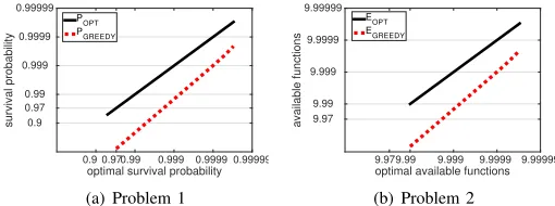
Fig. 4. Guarantees on the results of the greedy algorithm based on the optimal values. (a) Problem 1 withp= 10 10, (b) Problem 2 withp= 10 10,k= 10.
assigning each function to the partition with the largest product of failure probabilities so far.
This algorithm is equivalent to applying the well-known greedy algorithm for number partitioning, on inputs equal to minus the log of failure probabilities, similar to the reduction in Theorem 10. This algorithm is known to achieve7/6approximation of the size of the
larger partition [11]. One might ask how that known approximation ratio translates into guarantees on the effectiveness of the balancing algorithm, at least for this special case of c = 2 andk n= 2. Unfortunately, the result does not imply a fixed approximation ratio, but enables us to derive bounds on the performance of the greedy algorithm that vary for different instances.
Assume an instance with p =Qki=1pi for failure probabilities p1, . . . , pk. Let PCo1, P
o
C2 be the product of failure probabilities of
functions in the two connected components in an optimal solution such that POP T = (1 PCo1)·(1 P
o
C2) is the optimal survival
probability. We derive PGREEDY, a lower bound on the survival
probability of the greedy solution.
We denote PC1, PC2 the products corresponding to the two
connected components in the greedy solution. We assume w.l.o.g.
Po
C1 P
o
C2 andPC1 PC2. They satisfyP o C1·P
o
C2 =PC1·PC2 = p. The 7/6 approximation ratio on the size of the larger partition
in number partitioning gives us the following relation between
Po
C2 andPC2: PC2 (P o C2)
7/6. HerePo
C2 <1 and PC2 satisfies (Po
C2) 7/6
PC2 P o
C2. For a given value ofPOP T we solve the
two equations (1 Po
C1)·(1 P
o
C2) = POP T, P o C1 ·P
o
C2 = p
to derive Po
C2. The minimal survival probability is obtained by
the greedy algorithm when the lower bound on PC2 is tight and
PC2 = (P
o C2)
7/6. Then we can calculate P
C1 = p/PC2 and
PGREEDY = (1 PC1)·(1 PC2)as a function ofp, POP T.
In Figure 4(a) we demonstrate this by setting a constant p = 10 10, and leavingP
OP T, the survival probability of the optimal
solution, as an independent variable. We plot PGREEDY as a
function of POP T for this case, as well as the identity function
of POP T for comparison. Several points can be observed: • For low values of POP T, below roughly 0.97 in this case,
the value of PGREEDY is negative (hence not plotted in this
figure). This means that the approximation is too loose to be of any value.
• Above a certain value ofPOP T, there is no real solution for Po
C2, i.e., no real inputspi exist for this case. In our example
[image:8.612.319.574.53.148.2]between the bound on the probability of the greedy and the optimal one is improved (i.e., larger). For this example with
p= 10 10, the ratio is 0.9863 forP
OP T = 0.999and 0.9998
for POP T = 0.99997.
For Problem 2, very similar derivations apply. Here we need to assume as given, in addition topandEOP T, alsok, the number of
functions. We start fromEOP T =k PCo1 P o
C2, assume worst case
values forPC2 and derive a formula for EGREEDY as a function
of p,EOP T andk. Figure 4(b) plots this forp= 10 10, k= 10.
B. Calculating the value of an assignment
The number of possible assignments can be large, i.e. exponential in the number of servers and their capacity c. Moreover, for
both problems calculating the value of a given assignment, i.e. the survival probability in Problem 1 or the expected number of available functions in Problem 2 is not an easy task. The number of scenarios with different set of failed functions that have to be taken into account is 2k, i.e., exponential in the number of functions.
This often restricts the number of functions we can consider in the experimental settings. We develop dynamic-programming based techniques to accelerate this calculation. Basically, the approach is to go over all function subsets ordered by their subset size, maintaining the maximum matching size for each subset. An update of the maximum matching size of a subset A, with |A| = a, is
performed by the maximum matching size of all subsets of A of
sizea 1, and the number of adjacent servers ofA, using a simple
extension of Hall’s theorem [12].
C. Estimating Failure Probabilities
Our approach assumes that the failure probabilities of the mid-dleboxes are known. Of course, this information is not always easy to obtain. A recent study [1] examined for different middleboxes, the number of failures within a period of a year as well as the time it takes to repair them. We can use them as a guidelines to have some intuition on typical numbers. A mean number of 1.5-3.5 failures/year is described for 4 types of middleboxes such that roughly half of the failures are fixed within an hour but the 95th and the 99th percentiles are much longer and equal about 2.5 and 17.5 days, respectively. We use a conservative approach in the values we examine in the experimental settings selecting them uniformly over the range[0.025,0.175]where0.025⇡ 3.5·2.5
365 ,0.175⇡ 3.5·17.5
365 .
VII. EXPERIMENTALRESULTS
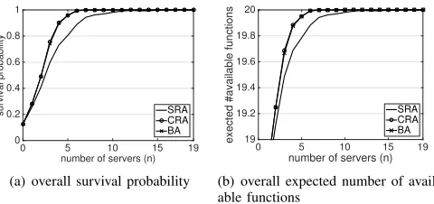
We now turn to evaluating our algorithms described in Section V. We first compare the different algorithms in Section VII-A, and then in Section VII-B we show the effect of the number of backups per server, c, on the number of servers required to achieve a
target survival probability. The simulation is based on the technique described in Section VI-B that computes the overall survival probability and expected number of available functions for a given backup assignment.
A. Competitive Evaluation
We first compare the algorithms proposed in Section V. Figure 5 shows the survival probability and the survival expec-tation, respectively, as a function of the number of servers. For the
number of servers (n)
0 5 10 15 19
survival probability
0 0.2 0.4 0.6 0.8 1
SRA CRA BA
(a) overall survival probability
number of servers (n)
0 5 10 15 19
exected #available functions 19 19.2 19.4 19.6 19.8 20
SRA CRA BA
(b) overall expected number of avail-able functions
Fig. 5. Performance comparison of the algorithms presented in Section V with
c= 4andk= 20.
Difference inP Difference inE
(Problem 1) (Problem 2)
n CRA BA CRA BA
9 5.58·10 3 4.39·10 3 5.66·10 3 4.48·10 3
10 8.50·10 4 4.10·10 4 8.55·10 4 4.16·10 4
11 7.33·10 5 1.67·10 5 7.34·10 5 1.68·10 5
12 7.61·10 6 6.23·10 7 7.61·10 6 6.30·10 7
13 3.90·10 7 2.20·10 8 3.90·10 7 2.00·10 8
TABLE I
COMPARISON OFCRAANDBAFOR LARGEn. THE TABLE SHOWS THE DIFFERENCE OF THE SURVIVAL PROBABILITYPFROM1AND THE DIFFERENCE
OF THE EXPECTED NUMBER OF AVAILABLE FUNCTIONSEFROMk= 20.
simulations in this section, we setk= 20,c= 4and compared the
algorithms asn, the number of servers, grows. To cope with the fact
that the algorithms performance depends on the actual input, and that some of the algorithms are random, we rely on average case analysis. Hence, for each n 2 {0,1,· · ·, k 1}, we created 100 random instances of failure probabilities vectors, where each failure probability is uniformly distributed over the range [0.025,0.175], selected by the considerations presented in Section VI-C.
As depicted in Fig. 5, the CRA and the BA algorithms outperform the SRA algorithm for all values of n. While their performance
seems similar, the CRA algorithm is slightly better than the BA algorithm when the number of servers is low. This is due to the fact that the BA algorithm balances the connected component probability based on their failure probabilities product, which is suitable for c = 2, while the CRA algorithm basically assigns
backups to the functions with the top mostc·nfailure probabilities
(for k c·n). However, this range of values for the number of
serversn is not of a much interest since it typically results in too
[image:9.612.329.569.52.165.2]low overall survival probability and expectation.
Table I distinguishes between the overall survival probability and expectation of the CRA and BA algorithms for relatively large values of n, when the survival probability and expectation obtain a reasonable value. The BA algorithm shows better results for all such values ofn.
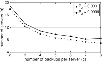
B. Effect of the number of backups per server
In this section we examine the effect of the number of backups per server, c. Figure 6 shows the number of servers required in
order to achieve a survival probability of 0.999 and 0.9999 as a function of the number of backups per server, c, where k = 20.
[image:9.612.328.566.200.282.2]number of backups per server (c)
2 3 4 5 6 7 8
number of servers (n)
4 8 12 16 20
[image:10.612.76.245.54.157.2]Pd = 0.999 Pd = 0.9999
Fig. 6. Number of servers needed to obtain a desired survival probabilityPdas a
function ofc, withk= 20functions.
simulations for eachc andk with 100 random instances of failure
probabilities vectors, distributed as in Section VII-A.
For example, Fig. 6 demonstrates that for 20 functions (i.e.k= 20), a survival probability of 0.999 requires 11 servers, each capable of backing up 4 functions (i.e.c= 4), or 10 servers, each backing up 5 functions (c = 5). Similarly, a 0.9999 survival probability requires 10 servers with a backup capacity of 5.
VIII. RELATEDWORK
Various studies have considered the design and implementation of high availability systems [2], [6], [13], [14]. Remus [2] and Colo [13] are general approaches offering fault tolerance for any VM-based system running a standard operating system.
Remus is based on checkpoint strategy recovering a failed system to the last saved state, while Colo is also based on parallel execution of identical VMs. Pico [14] was the first fault tolerance designated system for middleboxes. Its maintenance operates at the flow level state enabling lighter checkpoints. In [6], Fault-Tolerant MiddleBox system for rollback recovery is introduced employing ordered logging and parallel release for low overhead middlebox fault-tolerance. In [1], a large-scale empirical study of middlebox failures was performed in a service provider network showing that failures can significantly impact hosted services. These studies rely on middlebox redundancy, either in terms of checkpoint copies or parallel execution, while our study considers the crucial aspect of limited backup resources.
Similar to our work several works in NFV are based on resource allocation problems. In [15], known methods for solving the Gen-eralized Assignment Problem (GAP) [16] problem were employed in order to achieve a bi-criteria approximation to the performance of the virtual functions placement. In [17], the authors considered also the chaining policy constraints and proposed an Integer Linear Programming (ILP) model to allocate the virtual functions.
IX. CONCLUSIONS ANDFUTUREWORK
In this work we study how the flexibility of NFV can be leveraged for cost-effective survivable deployment of network functions. Following a formal analysis of two problems in this domain, we propose algorithms for computing an effective deployment, given the resource constraints. The algorithms are based on the intuitions obtained in the theoretical analysis of the problems. In a series of experiments, we show the effectiveness of these algorithms, and
demonstrate how high levels of survivability can be guaranteed with significant reduction in the amount of required resources.
This paper examines two specific optimization goals – the probability of full survival, and the expected number of operating functions following failures and recovery. Anther goals that can be considered is a deployment that fully guarantees recovery from a restricted small number of failed functions,t. One can also consider an online variant of the problem, where the failures are given one at a time. For each failure we are required toonlinechoose a server on which to run the function (out of those implementing the function), while trying to optimize some goal function globally. This is a variant of online matching in bipartite graphs. The difference here is that the edges to all left-hand-side nodes are known in advance, as well as the probability for each such node to appear in the input. One can also augment this problem by allowing the management system to update its backup scheme following each failure, with or without restrictions on the amount of changes allowed.
Acknowledgement:O. Rottenstreich was supported by the Roth-schild Yad-Hanadiv fellowship. J. Yallouz was supported by the Israeli Ministry of Science and Technology, by COST Action CA15127 RECODIS and was a summer intern in Nokia Bell-Labs.
REFERENCES
[1] R. Potharaju and N. Jain, “Demystifying the dark side of the middle: a field study of middlebox failures in datacenters,” inACM IMC, 2013.
[2] B. Cully, G. Lefebvre, D. T. Meyer, M. Feeley, N. C. Hutchinson, and A. Warfield, “Remus: High availability via asynchronous virtual machine replication,” inUSENIX NSDI, 2008.
[3] D. J. Scales, M. Nelson, and G. Venkitachalam, “The design of a practical system for fault-tolerant virtual machines,”Operating Systems Review, vol. 44, no. 4, pp. 30–39, 2010.
[4] M. Chiosi, D. Clarke, J. Feger et al., “Network Functions Virtualization. Introductory White Paper. ETSI, Darmstadt, Germany, October 2012.” [Online]. Available: http://portal.etsi.org/NFV/NFV White Paper.pdf [5] A. Gember, P. Prabhu, Z. Ghadiyali, and A. Akella, “Toward software-defined
middlebox networking,” inACM HotNets, 2012.
[6] J. Sherry, P. X. Gao, S. Basu, A. Panda, A. Krishnamurthy, C. Maciocco, M. Manesh, J. Martins, S. Ratnasamy, L. Rizzo, and S. Shenker, “Rollback-recovery for middleboxes,” inACM SIGCOMM, 2015.
[7] J. E. Hopcroft and R. M. Karp, “An n5/2 algorithm for maximum matchings in bipartite graphs,”SIAM J. Comput., vol. 2, no. 4, pp. 225–231, 1973. [8] B. G. Chandran and D. S. Hochbaum, “Practical and theoretical
improve-ments for bipartite matching using the pseudoflow algorithm,” CoRR, vol. abs/1105.1569, 2011.
[9] Y. Kanizo, D. Hay, and I. Keslassy, “Maximizing the throughput of hash tables in network devices with combined SRAM/DRAM memory,” IEEE Trans. Parallel and Distributed Systems, vol. 26, no. 3, pp. 796–809, 2015. [10] S. Mertens, “The easiest hard problem: Number partitioning,” in
Computa-tional Complexity and Statistical Physics, A. Percus, G. Istrate, and C. Moore, Eds. Oxford University Press, 2003, ch. 5, pp. 125–139.
[11] R. L. Graham, “Bounds on multiprocessing timing anomalies,”SIAM Journal of Applied Mathematics, vol. 17, no. 2, pp. 416–429, 1969.
[12] P. Hall, “On representatives of subsets,”J. London Math. Soc., vol. 10, no. 1, pp. 26–30, 1935.
[13] Y. Dong, W. Ye, Y. Jiang, I. Pratt, S. Ma, J. Li, and H. Guan, “COLO: coarse-grained lock-stepping virtual machines for non-stop service,” inACM SOCC, 2013.
[14] S. Rajagopalan, D. Williams, and H. Jamjoom, “Pico replication: a high availability framework for middleboxes,” inACM SOCC, 2013.
[15] R. Cohen, L. Lewin-Eytan, J. Naor, and D. Raz, “Near optimal placement of virtual network functions,” inIEEE Infocom, 2015.
[16] R. Cohen, L. Katzir, and D. Raz, “An efficient approximation for the gener-alized assignment problem,”Inf. Process. Lett., vol. 100, no. 4, pp. 162–166, 2006.