Conventional contracts, intentional behavior and logit choice:
Equality without symmetry
ISung-Ha Hwanga, Wooyoung Limb, Philip Nearyc, Jonathan Newtond,∗ aSogang University, Seoul, Korea.
bHong Kong University of Science and Technology cRoyal Holloway, University of London, England
dUniversity of Sydney, Australia
Abstract
When coordination games are played under the logit choice rule and there is intentional bias in agents’ non-best response behavior, the Egalitarian bargaining solution emerges as the long run social norm. Without intentional bias, a new solution, the Logit bargaining solution emerges as the long run norm. These results contrast with results under non-payoff depen-dent deviations from best response behavior, where it has previously been shown that the Kalai-Smorodinsky and Nash bargaining solutions emerge as long run norms. Experiments on human subjects suggest that non-best response play is payoff dependent and displays intentional bias. This suggests the Egalitarian solution as the most likely candidate for a long run bargaining norm.
Keywords: Evolution, Nash program, logit choice, egalitarianism. JEL Classification Numbers: C73, C78.
IFirst version: January 31, 2014. This version: September 4, 2016. S.-H.Hwang was supported by the National Research Foundation of Korea Grant funded by the Korean Government(NRF-2016S1A5A8019496). W. Lim was supported by a grant from the Re-search Grants Council of Hong Kong (Grant No. ECS-699613). Sincere thanks are given to Michihiro Kandori, Heinrich Nax, Bary Pradelski and Peyton Young for comments and suggestions.
∗Corresponding author.
Email addresses: [email protected](Sung-Ha Hwang),[email protected](Wooyoung Lim),
1. Introduction
Consider a two player coordination game with zero-payoffs for miscoordination and with payoffs on the main diagonal that correspond to points on the efficient frontier of a convex bargaining set. In his paper, ‘Conventional Contracts’, Young (1998a) showed that if pop-ulations of agents play such a game, usually updating their strategies according to a best response rule, but occasionally making an error and playing something other than a best response, then the long run social norm that emerges approximates theKalai and Smorodin-sky(1975) bargaining solution. Subsequently,Naidu, Hwang and Bowles(2010) showed that if errors are intentional so that an agent who makes an error always demands more than the best response, never less, then the Nash(1950) bargaining solution emerges as the long run social norm. The errors in the cited works are uniform – all possible errors are equally likely. However, there is another commonly used model of perturbed best response, thelogit
choice rule. Under logit choice, errors which incur a higher payoff loss for the agent making them are less likely to be made. The recent approximation results of Hwang and Newton
(2016) allow us to solve the problem of conventional contracts under logit choice.
It is shown that if the logit choice rule is used with intentional errors, then the Egalitarian bargaining solution (Kalai, 1977) emerges as the long run social norm. Justifications of Egalitarianism have usually assumed some symmetry in the problem faced (Alexander and Skyrms, 1999) or invoked ex-ante symmetry of players with respect to their position in the game (Binmore, 1998, 2005). One contribution of the current paper is to give a model of adaptive behavior that leads to the Egalitarian solution without any symmetry assumptions beyond those on population size and uniformity in matching.
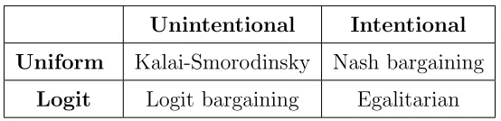
Unintentional Intentional
Uniform Kalai-Smorodinsky Nash bargaining Logit Logit bargaining Egalitarian
Table 1: Long run bargaining norms by error process. Each bargaining solution can be justified by the corresponding behavioral rule and without reference to any appealing ex-post properties that the solution might have.
comparison to the other solutions. This nonmonotonicity can be clearly and intuitively explained with reference to the underlying behavioral process, a good example of how a complex social norm can be generated by simple behavior.
Of course, the importance of the implications of any behavioral rule rests to some ex-tent on its empirical validity. To begin to address such questions we report the results of experiments conducted to test error behavior in the context of the model of the paper. We find evidence in favour of intentional bias and payoff dependence in non-best response play. While the constraints of time mean that we cannot test the long run behavior of the empirical process, these results, together with the theoretical results summarized in Table 1, suggest the Egalitarian solution as the most likely of our four candidates for a long run bargaining norm. Importantly, our design gives subjects no information about the payoffs that can be attained by their potential opponents, thereby ensuring that neither pre-existing norms of surplus division nor other-regarding preferences can play a role in strategy choice.
This study is part of theEvolutionary Nash Program, a literature that studies connections between evolutionary game theory and cooperative game theory.1 One well-developed strand of this literature concerns long run norms in Nash demand games.2 For two player Nash demand games, Young (1993b) shows that the Nash bargaining solution emerges, and for generalized Nash demand games, Agastya (1999) and Newton (2012b) find selection for minmax and maxmin (Rawlsian) solutions respectively. Another strand of the literature concerns selection in matching environments with either non-transferable utility (Newton and Sawa,2015) or transferable utility (Nax and Pradelski, 2014;Klaus and Newton,2016). Interestingly, although both Nax and Pradelski (2014) and Newton (2012b) find maxmin selection, these results arise in different ways. Nax and Pradelski (2014) use logit errors. Selection then comes from (i) how hard it is for a player to make errors. Newton (2012b) uses uniform errors and sampling of opponents’ behavior: selection comes from (ii) given an
1See
http://sharedintentions.net/research/evo-nash-program/for a discussion of the Evolution-ary Nash Program and the Shared Intentions Agenda.
2SeeBinmore, Samuelson and Young(2003) for a discussion of differences and similarities between Nash
incumbent strategy (a ‘convention’), the number of errors required to induce some player to respond with a different strategy. In the current study, we have that under logit choice, when errors are intentional, effect (ii) is dominated by effect (i). Consequently, the long run social norm is the convention at which it is least likely that any player makes an error. Under logit choice, this corresponds to the payoff of the poorest player being as high as possible - the Egalitarian solution. In contrast, when errors are unintentional, effects (i) and (ii) combine to create the interesting nonmonotonicities of the Logit bargaining Solution.
Our experiments contribute to a small literature that considers non-best response behav-ior in laboratory data as analagous to errors in best response dynamics. For two strategy coordination games, when interaction is determined by a network, M¨as and Nax(2016) find errors to be payoff dependent. When interaction is uniform, Lim and Neary (2016) find likewise. Furthermore, the cited studies find that errors are predominantly made by agents who do relatively badly at the current convention. This points towards errors being inten-tional. The current study has more than two strategies and is therefore able to provide more conclusive evidence on this point, as any given agent has several possible errors that he could make, some of which can be interpreted as intentional and others which cannot. We find that 83% of errors in our experiments can be interpreted as intentional.
The paper is organized as follows. Section2defines the bargaining solutions and gives the evolutionary model. Section 3 classifies bargaining solutions by the behavioral rules which give rise to them. Section 4 discusses our experimental evidence. Section5 concludes.
2. Model
2.1. Bargaining solutions
Consider two positions, α and β, and a closed, convex bargaining set S ⊂R2 containing the origin. The set S gives feasible payoffs for players in theα and β positions respectively. Let the bargaining frontier, the efficient points ofS, be given by a strictly decreasing, differ-entiable, and concave function, f : R → R, such that (t, f(t)) is the efficient payoff pair in which α and β players receive t and f(t), respectively. Normalizing the disagreement point to (0,0), the maximum payoff that playersα and β can obtain are
¯
sα := max{t :f(t)≥0} and s¯β := max{f(t) :t ≥0}.
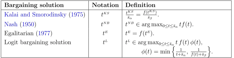
Bargaining solution Notation Definition
Kalai and Smorodinsky (1975) tKS tKS
¯
sα = f(tKS)
¯
sβ .
Nash (1950) tN B tN B ∈arg max
0≤t≤¯sαtf(t).
Egalitarian (1977) tE tE =f(tE).
Logit bargaining solution tL tL∈arg max
0≤t≤¯sαt f(t)φ(t),
φ(t) = minnt+¯1sα, f(t)+¯1 sβo.
Table 2: Bargaining solutions for frontiers given byf(.). Our assumptions onf(.) guarantee thatt f(t)φ(t) is strictly concave, sotL is unique.
appealing properties. The traditional approach is to treat these properties as axiomatic and to find bargaining solutions which have these properties. This is not the approach of the current paper. Rather, we focus on how solutions emerge as long run behavioral norms when agents follow simple behavioral rules when faced with coordination problems. That is, the behavior that gives rise to the solution is treated as axiomatic rather than the properties of the solution itself. Definitions of the bargaining solutions that feature in this paper are given in Table 2. The Logit bargaining solution, which is new, is analyzed further and compared to existing bargaining solutions in Section 3.1, but for now we move to define the perturbed best response rules that lead to these solutions emerging as norms.
2.2. Evolutionary contracting
Consider two populations of agents − α and β populations − of size N.3 Each period, all agents are uniformly matched in heterogeneous pairs of one α-agent and one β-agent to play a coordination game. The set of possible outcomes on which coordination is possible corresponds to a bargaining frontier as described in Section 2.1. Similarly to previous lit-erature, we discretize the bargaining frontier as follows. Let n ∈ N+, δ = δn = n−1s¯α, and I :={0,1,2,· · · , n} and suppose that α and β-agents play strategiesiα and iβ from setI.
We consider contract games (Young, 1998a), coordination games in which players who demand the same outcome receive their associated payoffs, and receive nothing otherwise. That is, the payoffs for a contract game are
(πα(iα, iβ), πβ(iβ, iα)) := (
(iδ, f(iδ)) if iα =iβ =i
(0,0) otherwise .
3Exposition is simplified by the assumption that the populations are of the same size. This is always the
Thus, when an α-agent plays i∈ I this can be interpreted as him demandingiδ, and when a β-agent plays i∈ I this can be interpreted as him demanding f(iδ).4
A population state is described by x:= (xα, xβ),where xα and xβ are vectors giving the
number of agents using each strategy. Thus, the state space Ξ is
Ξ :=
(
(xα, xβ)∈N0n+1×Nn0+1 :
X
l∈I
xα(l) = N, X
l∈I
xβ(l) = N )
.
More explicitly, we have (xα, xβ) = ((xα(0), xα(1),· · · , xα(n)),(xβ(0), xβ(1),· · · , xβ(n))),
where xβ(2),for example, denotes the number of β-agents playing strategy 2.
Agents from each population are uniformly matched to play the contract game and thus, the expected payoff of anαagent who plays strategyiαis πα(iα, x) :=Pl∈Iπα(iα, l)xβ(l)/N,
given that the fraction of theβ population using strategylisxβ(l)/N.Similarly, the expected
payoff of a β-agent who plays strategy iβ is πβ(iβ, x) := P
l∈Iπβ(iβ, l)xα(l)/N. Thus, the
best response of anα-agent to state xis to choose ito maximize πα(i, i)xβ(i), and the best
response of a β-agent is to choose i to maximize πβ(i, i)xα(i).
We consider the following discrete time strategy updating process. At the beginning of each period, any given agent is independently activated with probability ν ∈ (0,1). Any agent who is not activated will remain playing the same strategy as he did in the previous period. When the current population state isx, an activated agent in populationγ ∈ {α, β}
will choose a strategy according to the distribution pη
γ(l|x), l ∈ I. This distribution will be
such that an activated agent will usually choose a best response to the profile of strategies played by the opposing population. However, from time to time, an agent will make an
error and play something other than a best response. The parameter η parameterizes the probability of such errors, with larger values ofη corresponding to higher error probabilities. Asηapproaches zero, the probability of an error should approach zero at an exponential rate. Errors can be understood as occasional idiosyncratic experimentation, mistakes in play, or as atypical choices arising from random utility shocks. This paper considers processes with perturbations varying in two dimensions: the support of the error distribution (unintentional vs. intentional) and the payoff dependence or otherwise of errors within this support (uniform vs. logit).
4Note that the discretization is uniform for α, but not for β. This can be reversed without changing
Uniform mistake rule (see e.g. Young, 1993a; Kandori et al., 1993).
When errors are uniform, every error occurs with the same probability. That is, from state x, a strategy-revising agent from population γ ∈ {α, β} will choose l with probability
pηγ(l|x) :=
1
|arg max˜lπγ(˜l,x)|
(1−ε) + n+11 ε if l∈arg max˜lπγ(˜l, x)
1
n+1ε otherwise
whereε= exp(−η−1). Note, that as required above, as η→0, the probability of a strategy-revising agent playing anything other than a best response approaches zero.
Logit choice rule (see e.g. Blume, 1993, 1996; Al´os-Ferrer and Netzer, 2010).
Under the (generalized) logit choice rule, from state x, a strategy-revising agent from population γ ∈ {α, β} will choose strategy l with probability
pηγ(l|x) := qlexp(η −1π
γ(l, x)) P
˜
lq˜lexp(η−1πγ(˜l, x))
(1)
where ql, l ∈ I, are positive constants. Again note that as η → 0, the probability of a
strategy-revising agent playing anything other than a best response approaches zero.
Intentional & Unintentional errors (see e.g. Bowles, 2005, 2006; Naidu et al., 2010).
Let ∆γ(x) be the set of strategies for an agent of typeγ ∈ {α, β}which involve demanding
at least as much as the agent demands when best responding to the strategy distribution of the other population.
∆γ(x) := {l: πγ(l, l)≥πγ(l0, l0) for somel0 ∈arg max
˜
l
πγ(˜l, x)}.
Unintentional error processes retain the probabilities pη
γ(l|x) described above for logit and
uniform errors. Intentional errors are when agents never demand less than their best re-sponse, but can demand more. This fits with an interpretation of the perturbations as idiosyncratic experimentation by agents to see if they can obtain a higher payoff. There exists recent experimental evidence which supports such errors (Lim and Neary, 2016; M¨as and Nax, 2016). The choice probabilities for intentional processes are
ˆ
pηγ(l|x) :=
pηγ(l|x)
P
˜ l∈∆γ(x)p
η
γ(˜l|x) if l ∈∆γ(x)
0 otherwise
2.3. Conventions and long run social norms
The process with η= 0, or ε= 0, is theunperturbed process. The recurrent classes of the unperturbed process are the absorbing states in which all α andβ-agents coordinate on the same strategy, and each agent type receives nonzero payoff (Young,1998a). We shall denote by Ei, i ∈ {0, . . . , n}, the state in which all agents play strategy i, xα(i) = N, xβ(i) = N.
Hence, the absorbing states of the process are precisely those in the set {E1, . . . , En−1}. Following Young (1993a), we refer to these states as conventions. Let L := {1, . . . , n−1}
index this set, {Ei}i∈L.
We consider the long run behavior of our perturbed processes when errors are unlikely, that is as η → 0. For the current model, each process, uniform or logit, unintentional or intentional, for given η > 0, has a unique stationary distribution, which we denote µη
(see Lemma 1 in Appendix A). By standard arguments (see Young, 1998b), the limit µ:= limη→0µη exists, and for any x ∈ Ξ, µ(x) > 0 implies that x is in a recurrent class of the
process with η= 0. In our setting, this implies that x is a convention. Definition 1. A state x∈Ξ is stochastically stable if µ(x)>0.
For small error probabilities, in the long run, our processes will spend nearly all of the time at or close to stochastically stable states, hence the interpretation of such states as long run social norms. In the next section we link the stochastically stable states of our four processes to our four bargaining solutions.
3. Characterization
In this section we characterize the stochastically stable conventions. For a fine discretiza-tion (small δ) and large populations (large N), the stochastically stable conventions of our four processes correspond to our four bargaining solutions. The results for uniform errors are known fromYoung (1998a) and Naidu, Hwang and Bowles(2010). The results for logit errors are new.
Theorem 1. For any ς > 0, there exists ¯δ such that for all δ <δ¯, there exists Nδ ∈N such
that for all N ≥Nδ, µ(Ei)>0 =⇒ |δi−t∗|< ς, where
t∗ =
tKS if errors are uniform-unintentional.
tL if errors are logit-unintentional.
tN B
if errors are uniform-intentional.
tE if errors are logit-intentional.
played in error. From the perspective of a β-agent, the most attractive error that can be made by α-agents is for them to switch to strategy 0, as this opens up the possibility of
β-agents obtaining their highest payoff of ¯sβ by coordinating with such an α-agent. From
a convention Ei, δi = t, the number of such errors required to make the best response for
a β-agent differ from i depends on the ratio of the payoff from successful coordination on the current convention, f(t), to the highest payoff ¯sβ (see expression in Table 3). If f(t) is
small relative to ¯sβ, then few errors by α-agents will be required to escape the convention.
Reprising this argument, we see that if t is small relative to ¯sα, then few errors byβ-agents
will be required to escape the convention. Foruniformerrors, all possible errors are equally likely, so the difficulty of escaping a convention depends only on the number of errors required to change the best response. This number is maximized when the payoff ratios discussed above are equal: the Kalai-Smorodinsky solution.
When errors areintentional, agents who make errors will always ask for more than they receive at the current convention. From convention Ei, δi = t, from the perspective of a
β-agent, the most attractive error that can be made byα-agents is for them to ask for t+δ, just a little bit more than they currently receive. The number of errors required to change the best response ofβ-agents then depends on the ratiof(t+δ)/f(t)(see expression in Table3). This quantity (f(t+δ)/f(t)) and the equivalent quantity for transitions driven by errors of β -agents ((t−δ)/t) are respectively increasing and decreasing in t. For uniform errors, the most robust convention is thus where these quantities are equal: the Nash bargaining solution.
Forlogiterrors, to find the rareness of transitions the number of errors must be weighted by the payoff losses incurred when the errors are made. For intentional errors, as the dis-cretization becomes fine,f(t+δ)/f(t)→1 for all strictly positivet, so the number of α-agents who must make errors in order to alter the best response of β-agents will approach half. Likewise, the number of β-agents who must make errors in order to alter the best response of α-agents will also approach half. This means that the payoff loss effect dominates and the most robust conventions are those at which errors by either population are as rare as possible. This occurs when the payoffs ofαandβ players are equal: the Egalitarian solution.
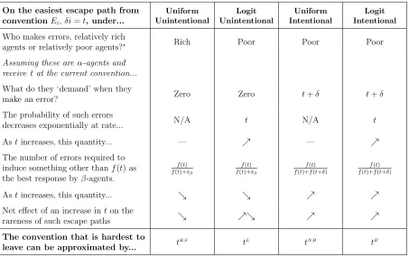
On the easiest escape path from conventionEi,δi=t, under...
Uniform Unintentional
Logit Unintentional
Uniform Intentional
Logit Intentional
Who makes errors, relatively rich
agents or relatively poor agents?∗ Rich Poor Poor Poor
Assuming these are α-agents and receive tat the current convention...
What do they ‘demand’ when they
make an error? Zero Zero t+δ t+δ
The probability of such errors
decreases exponentially at rate... N/A t N/A t
Astincreases, this quantity... — % — %
The number of errors required to induce something other thanf(t) as the best response byβ-agents.
f(t) f(t)+¯sβ
f(t) f(t)+¯sβ
f(t) f(t)+f(t+δ)
f(t) f(t)+f(t+δ)
Astincreases, this quantity... & & % %
Net effect of an increase inton the
rareness of such escape paths & %& % %
The convention that is hardest to
leave can be approximated by... t
KS tL tN B tE
Table 3: Anatomy of the easiest escape path from a given conventionEi,δi=t, by error process. ∗We write that errors are made byrelatively poor agents when there exists a threshold ˆt, such that fromEi,δi <ˆt, the easiest escape path involves errors byα-agents, and from Ei,δi >ˆt, the easiest escape path involves errors byβ-agents. When these inequalities are reversed, we write that errors are made byrelatively rich agents.
poor agents, in contrast to the uniform-unintentional case. The Logit bargaining solution is examined in depth in Appendix B. For now, attention is restricted to one part of the solu-tion as we examine the links between behavioural rules and the properties of the associated bargaining solutions.
3.1. The properties of the solutions as they relate to behavior
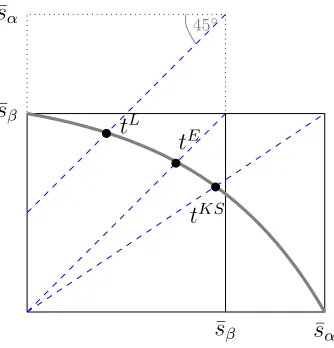
It is shown in Appendix B that the Logit bargaining solution reduces to a piecewise function, taking different forms dependent upon whether ¯sαis small, medium or large relative
to ¯sβ. Here we focus on the intermediate case, for which the solution is given by
tL
+ ¯sα =f(tL) + ¯sβ. (2)
This is an Egalitarian solution with a notional disagreement point of (¯sβ,s¯α) (see Figure 1).
45◦
tE
tKS
tL
¯
sα
¯
sβ
¯
sβ
¯
sα
Figure 1: The intermediate case (Case 2 inAppendix B) of the Logit bargaining solution, also illustrating Egalitarian and Kalai-Smorodinsky solutions for comparison.
Therefore interpersonal comparability of payoffs follows from interpersonal comparability of error rates. However, interpersonal comparability of payoffs is precisely what is prohibited under the Invariance property, so the solutions that emerge from logit choice (Logit bar-gaining solution, Egalitarian solution) do not satisfy Invariance. In contrast, under uniform errors, choice probabilities are unaffected by a linear transformation of an agent’s payoffs, so the solutions that emerge (Kalai-Smorodinsky, Nash) satisfy Invariance.
The presence of ¯sα and ¯sβ in expression (2) implies that the Logit bargaining solution
does not have the Independence of Irrelevant Alternatives property (IIA - Table 4). This is noteworthy, as under the logit choice rule, the ratios of choice probabilities pηγ(l|x)/pηγ(l0|x) are
independent of the payoffs from any strategy ˜l 6=l, l0. This shows that the IIA property at a micro level (choice behavior) does not translate into an IIA property at a macro level (long run social norm). The dependence of (2) on ¯sα and ¯sβ, and hence the failure of IIA, arises
from the fact that errors in the underlying behavioral process are unintentional. When error behavior is unintentional, the least cost transition paths between conventions involve jumps to extreme states motivated by the prospect of extreme payoffs (¯sα and ¯sβ), so the solutions
that emerge (Kalai-Smorodinsky, Logit bargaining solution) do not satisfy IIA. In contrast, when errors are intentional, least cost transition paths are between adjacent conventions and the solutions that emerge (Nash, Egalitarian) satisfy IIA.
Property Definition Satisfied by...
IIA g ≥f, g(t∗g)≤f(t∗g) =⇒ t∗g =t∗f. tN B, tE
Invariance g(x) =f(ax), a∈R =⇒ t∗g = 1at∗f. tN B, tKS
Monotonicity g ≥f =⇒ t∗g ≥t∗f. tE
Individual Monotonicity g ≥f, g(0) =f(0) =⇒ tg∗ ≥t∗f. tKS, tE
Stretch Monotonicity g(x) =f(ax), a∈R, a <1 =⇒ t∗g ≥t∗f. tN B, tKS, tE
Table 4: Definitions of properties and the bargaining solutions that satisfy them. In each definition, g, f
are bargaining frontiers and t∗
g, t∗f their associated solutions. Invariance implies Stretch Monotonicity, and Monotonicity implies Individual Monotonicity which implies Stretch Monotonicity. Note that tL satisfies none of these properties.
axis leads to the player in the α position obtaining a higher payoff (Stretch Monotonicity - Table 4). This property is implied by Invariance and Individual Monotonicity, and thus satisfied by the Egalitarian, Kalai-Smorodinsky and Nash solutions. However, we shall see that it is not satisfied by the Logit bargaining solution.
Consider a linear frontier given by f(t) = ¯sβ −t
¯
sβ
¯
sα. A stretch parallel to the horizontal
axis is equivalent to an increase in the value of ¯sα. Substituting the expression for the frontier
into (2), we obtain the solution tL= (2¯sβ−¯sα)¯sα
¯
sα+¯sβ . This is decreasing in ¯sα whenever ¯sα and ¯sβ
take similar values. That is, an increase in the best possible payoff for theα player leads to his obtaining a lower payoff under the Logit bargaining solution. This may seem puzzling at first, but makes sense when we consider that, under logit errors, the easiest escape path from a convention involves errors by relatively poor agents. Consider conventions for which
t > tL. These are the conventions at whichα-agents obtain high payoffs and from which the
most likely escape paths involve errors by β-agents. Under unintentional errors, the number of errors byβ-agents required to change the best response ofα-agents is lower when the best possible payoff ¯sα for α-agents is higher. That is, α-agents suffer from a high best possible
payoff as this destabilizes the conventions whereα-agents do well and pushes the value oftL
lower. See Appendix Bfor a complete illustrated solution for the linear bargaining frontier.
4. Experimental evidence for intentional and payoff dependent errors
α-player
β-player
1 2 3 4 5
1 0,100 0,0 0,0 0,0 0,0 2 0,0 80,80 0,0 0,0 0,0 3 0,0 0,0 130,65 0,0 0,0 4 0,0 0,0 0,0 180,50 0,0 5 0,0 0,0 0,0 0,0 200,0
1
Figure 2: Entries give payoffs for theαandβ players respectively.
the university graduate and undergraduate population. All sessions were conducted using z-Tree (Fischbacher,2007). Each session lasted for approximately two hours, and the average amount earned per subject was HKD 132 (USD 17), including the HKD 30 show-up fee.
Each session involved α and β populations of subjects (representing the agents in the model of Section 2) of size N = 10 playing for 200 periods. Each period, every subject, independently with probability ν (= 0.9 in Sessions 1,2,3; = 0.5 in Sessions 4,5), was activated and got the opportunity to update his strategy. The information displayed to a subject was:
(i) Hisown payoff when playing any given strategy and matched to a member of the other population also playing that strategy.
(ii) For periods τ ≥ 2, the number of subjects in the other population who played each strategy in the preceding period.
(iii) The strategy played and the payoff obtained by the subject in the preceding period. (iv) Whether or not the subject has the opportunity to update his strategy in the current
period.
Note that subjects were given no information about the coordination payoffs of subjects in the other population and the laboratory was set up to ensure that no subjects would gain any such information during the session.
Subjects given the opportunity to change their strategy could choose any of strategies 1 to 5, which were labeled asAtoE, the order of the labeling and the order of presentation of the strategies differing across sessions. If they were activated and failed to choose a strategy within a specified period, they remained playing the same strategy as in the previous period. Following strategy updating, α-subjects were paired with β-subjects and obtained payoffs corresponding to their chosen strategies played against one another in the game in Figure2. The instructions given to subjects and images of the decision making interface are given in
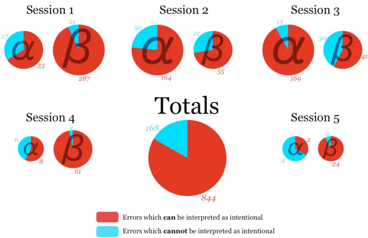
Figure 3: Chart showing, for each session and player position (α or β) in the game, the number of non-best responses that can be interpreted as intentional (those in ∆γ(x)) and that cannot be interpreted as intentional (those not in ∆γ(x)), as well as totals across all sessions and positions. The area of each pie chart is approximately proportional to the square root of the number of errors it represents.
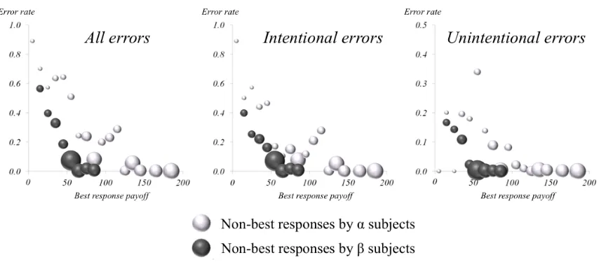
In every session, best responses constituted a large majority (> 90%) of choices by the subjects and play converged to a convention. Analysis of non-best response play reveals that subjects rarely update to strategies that correspond to payoffs lower than the payoff associated with their best response strategy (see Figure3). In every session-population pair except one (Session 5,α-subjects, with only 6 data points) errors which can be interpreted as intentional outnumber errors which cannot be so interpreted. In total, 844 out of 1012 errors (> 83%) can be interpreted as intentional. That is, there is clear support for intentional behavior in non-best response play. Methodologically, as the game has five strategies, rather than two as in recent similar studies (Lim and Neary, 2016; M¨as and Nax, 2016), for any given subject with a given best response there exist multiple non-best response strategies, and so we were able to classify observed errors as intentional or not on an individual basis.5 Furthermore, we observe higher rates of non-best response play from subjects for whom the expected payoff from the best response strategy is lower (Figure 4). That is, there is support for payoff dependence in non-best response play. From the Figure it can be seen
5In contrast, if there are only two strategies, then, for a given subject with a given best response, there
Figure 4: Rates of non-best response play grouped by expected payoff from the best response strategy. Data are grouped into bins by best response payoff (0 to 10, 10 to 20, etc.). The area of each circle on the chart is proportional to the square root of the number of strategy updating opportunities it represents.
that this is true across both α and β populations and holds regardless of whether errors can be interpreted as intentional. Note that although the charts appear similar, the vertical axis of the unintentional chart has a scale of half that of the the other charts, reflecting the relative number of errors of each type as discussed in the preceding paragraph.
An important aspect of our design is that α-subjects do not know the coordination pay-offs of β-subjects and vice versa. This brings two benefits. Firstly, the potential impact of other-regarding preferences is minimized, as any beliefs about the payoffs of the oppos-ing population would have to be inferred from behavior. Secondly, and we believe more importantly, subjects’ strategy choice cannot be influenced by pre-existing social norms. If subjects could observe the full payoff structure of the game, then a pre-existing norm such as the Kalai-Smorodinsky, Nash, Egalitarian or Logit solutions could encourage subjects to play i = 3,4,2,3 respectively. The outcome of the sessions suggests that subjects did not infer any correspondence between a pre-existing norm and the payoff structure of the game, as of the five sessions, three converged to convention E4 (Nash), while one converged to E3 (Kalai-Smorodinsky, Logit) and one to E2 (Egalitarian).
The observed short run convergence to some convention is predicted by the theoretical processes considered earlier in the paper. Note though that nothing can be inferred about long run norms from observing the conventions that were reached. For such an analysis, we would require observations over a longer timescale than is feasible within the constraints of the laboratory.6 However, Theorem 1 can be used to comment on long run norms by
extrapolating from the characteristics of observed non-best response behavior. Our observa-tions suggest that non-best response play is intentional and payoff dependent. Therefore, the theory suggests that, of the four solutions considered in this paper, the Egalitarian solution is the most likely candidate for a long run social norm.
5. Discussion
What has been presented here is a theory of the emergence of bargaining solutions as social norms that rests on behavior and not on the properties of the solutions themselves. Societal interactions take individual behavior as an input and give a social norm, or to put it another way, a social choice, as output. Thus, if we think of a society as similar to an organism with agency, we can regard the traditional, normative approaches to social choice as specifying behavioral rules for society itself, rather than for the individuals within society. As such, the results of the current paper and the rest of the Evolutionary Nash Program can be understood as a reconciliation of micro and macro behavioral theories.
But what of decision making that does not occur at the individual level, nor at the societal level? What if small groups exhibit collective agency and collaboratively adjust their behavior? In recent years there has been considerable work on collective agency in behavioral rules and its effect on social norms (Newton, 2012b,a; Newton and Angus, 2015;
Newton and Sawa, 2015; Angus and Newton, 2015; Sawa, 2014; Nax and Pradelski, 2014;
Klaus and Newton, 2016). In particular, Newton (2012a) features a result directly related to the current paper: if collective agency is added to the model of Young (1998a), then the Nash bargaining solution is the long run norm instead of the Kalai-Smorodinsky solution.
So it is clear that agency can affect norms. It seems intuitive that the opposite should also be true: the presence of well developed norms in a group should help members of the group to face new problems, take decisions and adjust their behavior as if they were of one mind. For example, taking our cue from the results of the current paper, given that Alice and Bob have successfully hunted an animal, they may well divide the meat equally without delay, deliberation or disputation. Such a norm makes it possible to determine, prior to a joint hunt, whether such a hunt will be beneficial to both parties, and thus whether it will take place at all. The modeling of two way influence between norms and agency is an interesting avenue for future research.
convention to another will usually require 6 or more errors in one of the populations. In a period in which all subjects in a given population have the opportunity to update their strategies, at error rates of 10% (the approximate frequency observed in this study), 6 or more errors will occur with a probability of less than
1/6000. Therefore to make a statement about long run norms using aggregate population data alone would
Appendix A. Proofs
Denote byPη(x, y) the transition probability from statexto statey. Define the resistance of such a transition, V (x, y), as
V(x, y) := lim
η→0−ηlnP
η(x, y) (A.1)
where V is defined over the set of all x, y ∈ Ξ such that Pηˆ(x, y) > 0 for some ˆη > 0 (see
Beggs,2005;Sandholm, 2010).
For uniform errors, V(x, y) equals the number of agents who switch to anything other than a best response.
V(x, y) = X
γ∈{α,β}
X
l /∈arg max˜lπγ(˜l,x)
max{yγ(l)−xγ(l),0}. (A.2)
For the logit choice rule,V(x, y) equals the best response payoff minus the payoff from the chosen strategy, summed over all updating agents.
V(x, y) = X
γ∈{α,β}
X
l∈I
max{yγ(l)−xγ(l),0}
max ˜
l
πγ(˜l, x)−πγ(l, x)
. (A.3)
Lemma 1. Each process, uniform or logit, unintentional or intentional, for given η > 0, has a unique stationary distribution, which we denote µη.
Proof. Note that for all x ∈ Ξ, n ∈ ∆α(x), so for all of our processes, from any x ∈ Ξ,
we have that Pη(x, y) > 0 for some y such that y
α(n) = N. From y, n is a best response
for any β-agent, so Pη(y, E
n)>0. Therefore, from any x ∈Ξ, with positive probability En
will be reached within two periods. As the state space is finite, standard results in Markov chain theory7 imply that for all η >0, Pη has a unique recurrent class and µ
η exists and is
unique.
In a similar way that V(·,·) measures the rarity of single steps in the process, we will use a concept, overall cost, that measures the rarity of a transition between any two states over any number of periods. Let P(x, x0) be the set of finite sequences of states {x1, x2, . . . , xT}
such that x1 =x, xT =x0 and for some ˆη >0, Pηˆ(xτ, xτ+1)>0, τ = 1, . . . , T −1.
Definition 2. The overall cost of a transition between x, x0 ∈Ξ is:
c(x, x0) := min {x1,...,xT}∈P(x,x0)
T−1
X
τ=1
V(xτ, xτ+1). (A.4)
If there is no positive probability path between x and x0 then let c(x, x0) = ∞. We shall be interested in the cost of transitions between conventions. In the current setting, this quantity is always finite. Denote the overall cost functions for the uniform-unintentional, logit-unintentional, uniform-intentional and logit-intentional processes by cU, cL, cU I, cLI
respectively.
Lemma 2. For c∈ {cU, cL, cU I, cLI}, i∈L, let
Fi :=
x∈Ξ : For some γ ∈ {α, β}, {i} 6= arg max
j∈I πγ(j, x)
.
Then, to calculate minx∈Fic(Ei, x) via the minimization in (A.4) it suffices to consider {x1, . . . , xT} ∈ P(E
i, x) such that, for τ < T, xτ and xτ+1 are identical except that for
some j ∈ I, γ ∈ {α, β}, xτ+1
γ (i) = xτγ(i)−1 and xτγ+1(j) = xτγ(j) + 1.
Proof. Let {x1, . . . , xT}, x1 =E
i,xT ∈Fi, be such that
min
x∈Fic(Ei, x) = T−1
X
τ=1
V(xτ, xτ+1). (A.5)
As V(., .) ≥ 0, we can, without loss of generality, assume that xt ∈/ F
i for t < T. For
t= 1. . . , T −1, for all γ ∈ {α, β}, define
yγ1 =x1γ,
yγt+1(j) =yγt(j) + max{xtγ+1(j)−xtγ(j),0} for j 6=i, yγt+1(i) = N −X
j6=i
yγt+1(j).
That is, {y1, . . . , yT} differs from {x1, . . . , xT} only in that all transitions to any j ∈ I at
t+ 1 are now by agents who played i at t.
Lett0be the smallesttsuch thatyt ∈Fi. t0 ≤T asyγT(i)≤xTγ(i),yγT(j)≥xTγ(j) forj 6=i,
xT ∈Fi implies yT ∈Fi. By (A.2) or (A.3), i /∈Fi implies V(yt, yt+1)≤V(xt, xt+1).
There-fore, ift0 < T, thenc(y1 =x1, yt0)≤Pt0−1
t=1 V(y
t, yt+1)≤Pt0−1
t=1 V(x
t, xt+1)<PT−1
t=1 V(x
t, xt+1), contradicting (A.5). So t0 =T and for allt < T, we have yt ∈/ F
i and
Now, if P γy
t+1
γ (i) < P
γy t
γ(i)−1, then take some j, γ such that yγt+1(j) > yγt(j) and
define yt+ to be identical toyt except that yt+
γ (i) =ytγ(i)−1 and yγt+(j) = yγt(j) + 1. Then,
by (A.2) or (A.3) we have
V(yt, yt+) +V(yt+, yt+1)≤V(yt, yt+1). (A.7) Now replace{y1, . . . , yt, yt+1, . . . , yT}with{y1, . . . , yt, yt+, yt+1, . . . , yT}and iterate this pro-cedure until we obtain {z1, . . . , zT0} such that z1 = y1, zT0 = yT, and either zt+1 = zt or P
γz t+1
γ (i) = P
γz t
γ(i)−1 fort = 1, . . . , T
0−1. Ifzt+1 =zt, thenV(zt, zt+1) = 0, so we omit such transitions and renumber our sequence{z1, . . . , zT˜}, which now satisfies the conditions
in the statement of the lemma. Now,
min
x∈Fic(Ei, x) |{z}≤
by defn ˜
T−1
X
τ=1
V(zτ, zτ+1) ≤ |{z}
by iterating (A.7)
T−1
X
τ=1
V(yτ, yτ+1)
≤ |{z} by (A.6) T−1 X τ=1
V(xτ, xτ+1) =
|{z}
by (A.5) min
x∈Fic(Ei, x).
which completes the proof. Lemma 3. For i∈L,
cU(Ei, Ej) = min
N f(δi) f(δi) + ¯sβ
,
N δi δi+ ¯sα
for all j 6=i, (A.8)
cL(Ei, Ej)≈min
δi
N f(δi) f(δi) + ¯sβ
, f(δi)
N δi δi+ ¯sα
for all j 6=i, (A.9) min
j6=i c U I(E
i, Ej) = min
N f(δi)
f(δ(i+ 1)) +f(δi)
,
N i
2i−1
, (A.10)
min
j6=i c LI(E
i, Ej)≈min
δi
N f(δi)
f(δ(i+ 1)) +f(δi)
, f(δi)
N i
2i−1
. (A.11)
where a≈b denotes |a−b| ≤max{¯sα,s¯β}.
Proof. Let ξiγ be the lowest number of errors by a γ-agent, γ ∈ {α, β}, on any transition path from Ei,i∈L, to some Ej, j ∈ I,j 6=i. At some point on any such path, some j 6=i
must become a best response. Therefore,
ξαi max
j∈Cα i
πβ(j, j)≥(N −ξiα)πβ(i, i) and ξβi max j∈Ciβ
πα(j, j)≥(N −ξiβ)πα(i, i),
It follows that ξα
i is attained when α-agents make errors and play k ∈arg maxj∈Cα
i πβ(j, j),
and ξiβ is attained when β-agents make errors and play k∈arg maxj∈Cβ
i πα(j, j).
ξαi = min
j∈Cα i
N πβ(i, i) πβ(i, i) +πβ(j, j)
and ξiβ = min
j∈Ciβ
N πα(i, i) πα(i, i) +πα(j, j)
.
(A.12) Now, πα(i, i) = δi and πβ(i, i) = f(δi). For unintentional processes
max
j∈Cα i
πβ(j, j) = ¯sβ and max j∈Ciβ
πα(j, j) = ¯sα, (A.13)
and for intentional processes max
j∈Cα i
πβ(j, j) = f(δ(i+ 1)) and max j∈Ciβ
πα(j, j) =δ(i−1). (A.14)
For uniform errors, each error adds 1 to the cost of the transition, therefore the least cost transition from Ei, i ∈ L, to some Ej, j ∈ I, j 6=i, is one involving the fewest errors. The
cost of such a transition is then min{ξiα, ξiβ}, which by (A.12) and (A.13), equals the RHS of (A.8) for unintentional errors, and by (A.12) and (A.14), equals the RHS of (A.10) for intentional errors.
For logit errors, as each error is weighted by the expected payoff loss, the lowest cost from the transitions involving the fewest errors is min{πα(i, i)ξiα, πβ(i, i)ξiβ}. There may
exist lower cost transitions, but as Lemma 2 tells us we can restrict attention to paths in which one agent switches at a time, we can invoke Theorem 1 of Hwang and Newton(2016) and, for intentional processes, Theorem 1 from Hwang and Newton(2014), to give
min
j6=i c(Ei, Ej)≥min{πα(i, i)(ξ α
i −1), πβ(i, i)(ξiβ −1)},
so we have the RHS of (A.9) and (A.11).
Finally, note that for unintentional errors, by (A.13), lowest cost transitions out of Ei
involve extreme errors in which either α-agents switch to 0 until 0 is a best response for
β-agents, orβ-agents switch to n untiln is a best response forα-agents. Consider α-agents making errors until 0 is a best response for β-agents. It is then possible that all β-agents update their strategy to 0, to reach a state x such that xβ(0) =N. From such a state, any
arbitrary k without further mistakes. That is, c(Ei, Ek) = minj6=ic(Ei, Ej) for all k6=i.
The next step is to characterize the stochastically stable states of our model for given δ
and large population size.
Definition 3. The following expressions are the limits of 1/N multiplied by (A.8), (A.9),
(A.10), (A.11) as N → ∞, written as a function of t=δi.
ϕUδ(t) := min
f(t)
f(t) + ¯sβ
, t t+ ¯sα
,
ϕLδ(t) := min
t f(t) f(t) + ¯sβ
, f(t) t
t+ ¯sα
,
ϕU Iδ (t) := min
f(t)
f(t+δ) +f(t),
t
2t−δ
,
ϕLIδ (t) := min
t f(t)
f(t+δ) +f(t), f(t)
t
2t−δ
.
Lemma 4. For c∈ {cU I, cLI} and correspondingφ
δ ∈ {φU Iδ , φLIδ }, let i∈arg maxj∈Lϕδ(jδ).
Then
φδ(jδ) = lim N→∞
1
Nc(Ej, Ej+1) for j < i, φδ(jδ) = lim
N→∞ 1
Nc(Ej, Ej−1) for j > i.
Proof. We can write φδ(t) = min{a(t), b(t)}. Asa(t) is increasing int, b(t) is decreasing in
t, a(iδ)≤b(iδ) implies
a(jδ)< b(jδ) for j < i,
a(jδ)> b(jδ) for j > i. [otherwise φδ(jδ)> φδ(iδ), contradicting i∈arg max
j∈L ϕδ(jδ)]
If a(iδ)> b(iδ), a similar argument implies the same conclusion. To conclude, note that by the proof of Lemma 3,
a(jδ)< b(jδ) =⇒ lim
N→∞ 1
Nc(Ej, Ej+1) = limN→∞ 1
N mink6=j c(Ej, Ek) =φδ(jδ),
a(jδ)> b(jδ) =⇒ lim
N→∞ 1
Nc(Ej, Ej−1) = limN→∞ 1
N mink6=j c(Ej, Ek) =φδ(jδ).
a graph g, let (j →k)∈g denote an edge from j to k in g. Define stochastic potential:
SP(i) := min
g∈G(i)
X
(j→k)∈g
c(Ej, Ek). (A.15)
We know from Freidlin and Wentzell(1984, chap.6), Young(1993a) that:
µ(Ei)>0⇔i∈arg min
j∈L SP(j).
Lemma 5. For c∈ {cU, cL, cU I, cLI} and correspondingφ
δ ∈ {φUδ, φLδ, φU Iδ , φLIδ }, there exists
Nδ such that for all N ≥Nδ, µ(Ei)>0 =⇒ i∈arg maxj∈Lϕδ(jδ)
Proof. Let l /∈ arg maxj∈Lϕδ(jδ) and let i ∈ arg maxj∈Lϕδ(jδ). Consider g ∈ G(i). For
c = cU, cL, let g = {j → i : j ∈ L, j =6 i}. For c = cU I, cLI, let g = {j → j + 1 :
j ∈ L, j < i} ∪ {j → j −1 : j ∈ L, j > i}. Note that (j → k) ∈ g correspond to
c(Ej, Ek) that solve minkc(Ej, Ek). For c= cU I, cLI, this follows from the proof of Lemma
3, i ∈ arg maxj∈Lϕδ(jδ), and the fact that one term inside the minimization defining the
correspondingϕδ(t) is increasingt, the other term decreasing int. Thus (j →k)∈g implies
that limN→∞ N1c(Ej, Ek) = ϕδ(jδ). We have
lim
N→∞ 1
NSP(l) |{z}≥
by defn lim N→∞ 1 N X
j6=l j∈L
min
k6=j k∈L
c(Ej, Ek) = |{z}
by Lemma3and
1
Nmax{¯sα,¯sβ}→0
asN→∞
X
j6=l j∈L
ϕδ(jδ)
>
|{z}
byϕδ(lδ)<ϕδ(iδ)
X
j6=i j∈L
ϕδ(jδ) = |{z}
by Lemmas3,4 lim
N→∞ 1
N
X
(j→k)∈g
c(Ej, Ek) ≥ |{z}
by defn ofSP(i)
lim
N→∞ 1
NSP(i).
By (A.15), this shows that for large enough N, if l ∈ L does not maximize ϕδ(·δ) then
µ(El) = 0. So µ(Ei)>0 must imply that i∈arg maxj∈Lϕδ(jδ).
This characterizes the stochastically stable states for large N. The principle theorem of the paper approximates these states for small δ, linking them to bargaining solutions. To prove the Theorem we use the following lemma.
Lemma 6. Suppose ϕ is a continuous function which admits a unique maximum. Sup-pose ϕδ such that ϕδ converges uniformly to ϕ as δ → 0. Let t∗ ∈ arg maxϕ(t) and
i∗ ∈ arg maxiϕδ(iδ). Then for all ς > 0, there exists ¯δ > 0 such that for all δ < δ,¯ we
have |i∗δ−t∗|< ς.
Proof. By the definitions of t∗ ∈ arg maxtϕ(t) and i∗ ∈ arg maxiϕδ(iδ), we have ϕ(t∗) ≥
that |ϕδ(t∗)−ϕ(t∗)| < ς and |ϕδ(i∗δ)−ϕ(i∗δ)| < ς. For δ < δ,¯ we have ϕ(i∗δ) ≤ ϕ(t∗) ≤
ϕδ(t∗) +ς ≤ϕδ(i∗δ) +ς < ϕ(i∗δ) + 2ς. Thus we have that
For all ˜ς >0, there exists ¯δ such that for all δ <δ,¯ we have |ϕ(t∗)−ϕ(i∗δ)|<ς.˜ (A.16) Without loss of generality we suppose that i∗δ < t∗ and let ς >0 be given. Then for ς >0 we can choose ¯ρ such that for all ρ <ρ¯
ϕ(t∗)−ρ < y < ϕ(t∗) implies |ϕ−1(y)−t∗|< ς, (A.17) where ϕ−1 is the inverse function for ϕ defined in a neighborhood of t∗ except t∗. Now let
ς > 0. Choose ¯ρ satisfying (A.17) first. Then for ˜ς = ρ < ρ,¯ choose ¯δ satisfying (A.16). Then for ρ and for δ <δ,¯ we have |ϕ(i∗δ)−ϕ(t∗)|< ρ. Also sinceρ <ρ,¯ by (A.17) we have
|i∗δ−t∗| < ς. Thus we show that for allς > 0,there exists ¯δ > 0 such that for allδ <δ,¯ we have|i∗δ−t∗|< ς.
Proof of Theorem 1. Taking the limit of ϕU
δ(t) and ϕLδ(t) as δ →0 gives uniform convergence to
ϕU(t) := min
f(t)
f(t) + ¯sβ
, t t+ ¯sα
, (A.18)
ϕL(t) := min
t f(t) f(t) + ¯sβ
, f(t) t
t+ ¯sα
, (A.19)
respectively. These functions are maximized at tKS
, tL
, respectively. Lemmas 5 and 6 then complete the proof for the cases of uniform-unintentional and logit-unintentional errors.
For the case of logit-intentional errors, ϕLI
δ (t) takes the form min{a(t), b(t)}, with a(t) =
tf(t+fδ()+t)f(t) and b(t) =f(t)2tt−δ. Continuity off(·) implies that there exist ς >0, ˆδ >0 such that for all δ <δˆ, a(t)< b(t) for all δ ≤ t < ς, and a(t) > b(t) for all ¯sα−δ ≥ t > ¯sα−ς.
Therefore, the following function equals ϕLI
δ (t) at all t=δi, i= 1, . . . , n−1.
ˆ
ϕLIδ (t) =
a(t) if t < ς.
min{a(t), b(t)} if ς ≤t ≤s¯α−ς.
b(t) if t >s¯α−ς.
As δ→0, ˆϕLIδ converges uniformly to
ˆ
ϕLI(t) := min
t
2,
f(t) 2
This expression is maximized at tE. Lemmas 5 and 6 then complete the proof for
logit-intentional errors.
For the case of uniform-intentional errors, we cannot apply Lemma 6, since the ϕU I δ (t)
does not converge to a function with a unique maximum as δ → 0. However, in the mini-mization that definesϕU I
δ (t), one of the terms is increasing in t, the other is decreasing in t,
and they intersect at a unique ˜t. Therefore, for small δ,i∗ ∈arg maxi∈LϕU Iδ (iδ) is close to ˜t,
which is given by ˜
t
2˜t−δ =
f(˜t)
f(˜t+δ) +f(˜t) ⇔ ˜
tf(˜t+δ)−f(˜t)
δ +f(˜t) = 0,
which approaches the first order condition fortN B asδ →0. Henceδi∗ →tN B (See detailed argument in Naidu, Hwang and Bowles,2010).
Appendix B. The Logit bargaining solution
The definition of tL
in Table 2can be rewritten as
tL
= arg max
0≤t≤¯sαmin{h1(t), h3(t)}, h1(t) :=
tf(t)
f(t) + ¯sβ
, h3(t) :=
tf(t)
t+ ¯sα
. (B.1)
We denote the maximizers of h1(t),h3(t) by t1, t3 respectively.
tl := arg max
0≤t≤¯sαhl(t), l= 1,3.
When h1(t) andh3(t) intersect for 0≤t≤s¯α, that is for 12 ≤ ¯sα¯sβ ≤2, we let t2 be the value of t for which this intersection occurs. That is, t2 solves
t2+ ¯sα =f(t2) + ¯sβ. (B.2)
Remark 1. The Logit bargaining solution solves
tL
:=
t1 if h1(t1)< h3(t1), (Case 1)
t3 if h3(t3)< h1(t3) , (Case 3)
t2 otherwise. (Case 2)
The cases of the solution are numbered by the order in which they occur as the ratiosα¯ /¯sβ moves from low to high values. For low values ofsα¯ /¯sβ, the maximum ofh
Case Condition Solution 1 ¯sα <
3√2 2 −1
−1
¯
sβ tL= (2− √
2)¯sα
2 3
√ 2 2 −1
−1
¯
sβ ≤s¯α ≤
3√2 2 −1
¯
sβ tL=
(2¯sβ−¯sα)¯sα
¯
sα+¯sβ
3 ¯sα >
3√2 2 −1
¯
sβ tL= (
√
2−1)¯sα
Table B.5: Explicit expressions for the Logit bargaining solution when the frontier is linear.
In Case 1 and Case 3, the Logit solution is similar to the Nash solution, but adjusted to take into account the best possible outcome for one of the players. Comparing the first order condition for the Nash bargaining solution:
tN B
f0(tN B
) +f(tN B
) = 0
to the first order conditions for the Logit bargaining solution in Cases 1 and 3 respectively:
tL
f0(tL
) + s¯β +f(t
L)
¯
sβ
f(tL
) = 0, tL
f0(tL
) + s¯α
tL+ ¯s α
f(tL
) = 0.
we see that Player αobtains more in Case 1 and less in Case 3 than he does under the Nash solution. Moreover, in Case 3, an increase in ¯sαresults in Playerα achieving a higher payoff.
This increase of Player α’s payoff in his best possible payoff differs from the similar effect in the Kalai-Smorodinsky solution. The effect in the latter depends on the ratio of ¯sα and ¯sβ,
whereas in Case 3 of the Logit solution, changes in ¯sβ have no direct effect. Symmetrically,
in Case 1 the solution depends on f(.) and ¯sβ, but not directly on ¯sα.
When conditions for Case 2 are satisfied we see from Equation (B.2) and the illustration in Figure 1 that Player γ’s payoff decreases with ¯sγ. In fact, the solution is an Egalitarian
solution with a notional disagreement point of (¯sβ,s¯α). The disagreement point is wholly
notional as it lies outside of the bargaining set. The players equalize their losses from this notional disagreement point. This notional disagreement point for a player is equal to the maximum attainable payoff of the other player (see Figure1).
Now consider a linear bargaining frontier given by the equation f(t) = ¯sβ −t
¯
sβ
¯
sα.
Condi-tions under which each case of the solution pertains and explicit soluCondi-tions for each case are given in Table B.5. An increase in ¯sα is equivalent to a stretch of the bargaining frontier
parallel to the horizontal axis. It can be seen that when Case 2 pertains, an increase in ¯sα
results in a reduction in tL. Figure B.5 shows how, fixing ¯s
β, the payoff of Player α varies
0.5 1.0 1.5 2.0 0.2
0.4 0.6 0.8
Figure B.5: tL by ¯s
α, keeping ¯sβ= 1.
Appendix C. Experiments - instructions and interface
Appendix C.1. Decision screen faced by subjects
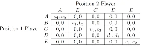
Here we give the decision screen faced by subjects from the second round onwards. Po-sition 1 corresponds to the population of α-subjects and Position 2 corresponds to the population of β-subjects. Subjects were informed of their own payoffs from successful coor-dination and the proportions of subjects in the other position who played each strategy in the preceding round.
Appendix C.2. Instructions given to participants
INSTRUCTIONS
Welcome to the study. In the following two hours, you will participate in 200 rounds of strategic decision making. Please read these instructions carefully; the cash payment you will receive at the end of the study depends on how well you perform so it is important that you understand the instructions. If you have a question at any point, please raise your hand and wait for one of us to come over. We ask that you turn off your mobile phone and any other electronic devices. Communication of any kind with other participants is not allowed.
Your Cash Payment
For each participant, the experimenter randomly and independently selects 3 rounds to calculate the cash payment. (So it is in your best interest to take each round seriously.) Each round has an equal chance to be selected as a payment round for you. You will notbe told which rounds are chosen to be the payment rounds for you until the end of the session. Your total cash payment at the end of the experiment will be the average earnings in the three selected rounds (translated into HKD as the exchange rate of 1 Token = 1 HKD) plus a 30 HKD show-up fee.
Your total cash payment = HK$ (The average of earnings in the 3 selected rounds) + HK$30
Your Role and Decision Group
You are one of 20 participants in today’s session. At the beginning of the experiment, one half of the participants will be randomly assigned to be in Position 1 and the other half to be in Position 2. Your position will remain fixed throughout the experiment. In each round, all individuals arerandomly paired so that each pair comprises one Position 1 player and one Position 2 player. Thus, in a round you will have an equal, 1 in 10 chance of being paired with any given participant in the other position. You will not be told the identity of the participant you are paired with in any round, nor will that participant be told your identity—even after the end of the experiment. Participants will be randomly re-paired after each round to form new pairs.
Your Decision in Each Round
made by you and the other participant are the same, may you be able to get a positive earning in the round.
Figure 1: Your Earnings
In words this says,
1. When you are a Position 1 player , if you and the other participant you are paired with have different actions, you each get 0. If you and the other player in your pair both choose
(a) Action ‘A’, you get a1 and the other getsa2, (b) Action ‘B’, you get b1 and the other gets b2,
(c) Action ‘C’, you get c1 and the other getsc2, (d) Action ‘D’, you get d1 and the other getsd2, and
(e) Action ‘E’, you get e1 and the other getse2.
2. When you are a Position 2 player, if you and the other participant you are paired with have different actions, you each get 0. If you and the other player in your pair both choose
(a) Action ‘A’, you get a2 and the other getsa1, (b) Action ‘B’, you get b2 and the other gets b1,
(c) Action ‘C’, you get c2 and the other getsc1, (d) Action ‘D’, you get d2 and the other getsd1, and
(e) Action ‘E’, you get e2 and the other getse1.
Do You Know Your Payoffs?
At the beginning of the first round, you will be assigned to a position. Then the payoff values, a1, b1, c1,d1, and e1, are revealed to the position 1 players and the payoff values, a2,
b2, c2, d2, and e2, are revealed to the position 2 players. However, you will not be told the payoff values for the players in the other position, even after the end of the experiment.
An Opportunity to Change Your Action
In the first round, every participant is given the opportunity to choose an action out of the five available ones. In any round from the second round, the opportunity to change an action is given to each participant independently with 90% chance only. That is, with 10% chance, any given participant is not allowed to change his/her action. In case that the opportunity to change your action is not given, you will see the following message in your decision screen:
“In this round, you are not given the opportunity to change your action choice.” and will be assigned the same action as in the previous round. You will not be told whether the opportunity to change an action is given to the participant you are paired with, nor will the participant you are paired with be told whether such an opportunity is given to you.
Information Feedback
In each round, at the right-bottom corner of your screen, you will see the summary of the previous round. First, you will see your action choice and your earning from the previous round. Second, you will see the bar chart that reports how many people among the 10 participants in the other position chose each action in the previous round.
Rundown of the Study
1. At the beginning of the first round, you will be assigned to a position, and you will be shown the payoff values for yourself. In the main panel of your decision screen, you will be prompted to enter your choice of action. You must choose one of five actions
A, B, C,D, and E within 30 seconds. If you do not choose an action, one action will be randomly assigned to you.
3. You will be prompted to enter your choice of action for the second round, if you have the opportunity to change your action. The game does not change, so as before you must choose one of five actions.
All future rounds are identical to the first round except for twoimportantdifference. (a) The first difference concerns how much time you have to choose an action. In rounds 2−10, you have 20 seconds to make a decision. If you do not make a deci-sion within the 20 second window, then you will be assigned whatever action you used in the previous round. For rounds 11−200, you have only 10 seconds in which to make a decision. Again, if you fail to choose an action in this timeframe, you will be assigned the same action as in the previous round.
(b) The second difference concerns whether the opportunity to change your action is given with 100% chance (round 1) or with 90% chance (rounds 2−200).
Administration
Your decisions as well as your cash payment will be kept completely confidential. Re-member that you have to make your decisions entirely on your own; do not discuss your decisions with any other participants.
Upon completion of the study, you will receive your cash payment. You will be asked to sign your name to acknowledge your receipt of the payment. You are then free to leave.
If you have any questions, please raise your hand now. We will answer questions individ-ually. If there are no questions, we will begin with the study.
Quiz
1. Suppose that you are a Position 1 player, and choose actionA. It turns out that the participant you are paired with chooses actionB. What is your earning?
Bibliography
Agastya, M., 1999. Perturbed adaptive dynamics in coalition form games. Journal of Eco-nomic Theory 89, 207–233.
Alexander, J., Skyrms, B., 1999. Bargaining with neighbors: Is justice contagious? The Journal of Philosophy 96, 588–598.
Al´os-Ferrer, C., Netzer, N., 2010. The logit-response dynamics. Games and Economic Behavior 68, 413–427.
Angus, S.D., Newton, J., 2015. Emergence of shared intentionality is coupled to the advance of cumulative culture. PLoS Comput Biol 11, e1004587. doi:10.1371/journal.pcbi. 1004587.
Beggs, A., 2005. Waiting times and equilibrium selection. Economic Theory 25, 599–628.
doi:10.1007/s00199-003-0444-6.
Binmore, K., 2005. Natural justice. Oxford University Press.
Binmore, K., Samuelson, L., Young, P., 2003. Equilibrium selection in bargaining models. Games and Economic Behavior 45, 296 – 328. doi:10.1016/S0899-8256(03)00146-5. Binmore, K.G., 1998. Game theory and the social contract: just playing. volume 2. MIT
press.
Blume, L.E., 1993. The statistical mechanics of strategic interaction. Games and Economic Behavior 5, 387 – 424. doi:10.1006/game.1993.1023.
Blume, L.E., 1996. Population Games. Working Papers 96-04-022. Santa Fe Institute. Bowles, S., 2005. Is inequality a human universal?, in: Barrett, C.B. (Ed.), The social
economics of poverty. Routledge, pp. 125–145.
Bowles, S., 2006. Institutional poverty traps, in: Bowles, S., Durlauf, S.N., Hoff, K. (Eds.), Poverty traps. Princeton University Press, pp. 116–138.
Fischbacher, U., 2007. z-tree: Zurich toolbox for ready-made economic experiments. Exper-imental economics 10, 171–178.
Hwang, S.H., Newton, J., 2014. A classification of bargaining solutions by evolutionary origin. Working Papers 2014-02. University of Sydney, School of Economics.
Hwang, S.H., Newton, J., 2016. Payoff-dependent dynamics and coordination games. Eco-nomic Theory doi:10.1007/s00199-016-0988-x.
Kalai, E., 1977. Proportional solutions to bargaining situations: Interpersonal utility com-parisons. Econometrica 45, pp. 1623–1630.
Kalai, E., Smorodinsky, M., 1975. Other solutions to nash’s bargaining problem. Economet-rica 43, 513–18.
Kandori, M., Mailath, G.J., Rob, R., 1993. Learning, mutation, and long run equilibria in games. Econometrica 61, 29–56.
Klaus, B., Newton, J., 2016. Stochastic stability in assignment problems. Journal of Mathe-matical Economics 62, 62 – 74. doi:http://dx.doi.org/10.1016/j.jmateco.2015.11. 002.
Lim, W., Neary, P.R., 2016. An experimental investigation of stochastic adjustment dynam-ics. Technical Report. Hong Kong University of Science and Technology.
M¨as, M., Nax, H.H., 2016. A behavioral study of noise in coordination games. Journal of Economic Theory 162, 195 – 208. doi:http://dx.doi.org/10.1016/j.jet.2015.12.010. Naidu, S., Hwang, S.H., Bowles, S., 2010. Evolutionary bargaining with intentional idiosyn-cratic play. Economics Letters 109, 31 – 33. doi:DOI:10.1016/j.econlet.2010.07.005. Nash, John F., J., 1950. The bargaining problem. Econometrica 18, pp. 155–162.
Nax, H.H., Pradelski, B.S.R., 2014. Evolutionary dynamics and equitable core selection in assignment games. International Journal of Game Theory 44, 903–932. doi:10.1007/
s00182-014-0459-1.
Neary, P.R., 2012. Competing conventions. Games and Economic Behavior 76, 301–328. Newton, J., 2012a. Coalitional stochastic stability. Games and Economic Behavior 75,
842–54. doi:http://dx.doi.org/10.1016/j.geb.2012.02.014.
Newton, J., Angus, S.D., 2015. Coalitions, tipping points and the speed of evolution. Journal of Economic Theory 157, 172 – 187. doi:http://dx.doi.org/10.1016/j.jet.2015.01. 003.
Newton, J., Sawa, R., 2015. A one-shot deviation principle for stability in matching problems. Journal of Economic Theory 157, 1 – 27. doi:http://dx.doi.org/10.1016/j.jet.2014. 11.015.
Sandholm, W.H., 2010. Population games and evolutionary dynamics. Economic learning and social evolution, Cambridge, Mass. MIT Press.
Sawa, R., 2014. Coalitional stochastic stability in games, networks and markets. Games and Economic Behavior 88, 90–111.
Shiryaev, A.N., 1995. Probability (2nd ed.). Springer-Verlag New York, Inc., Secaucus, NJ, USA.
Young, H.P., 1993a. The evolution of conventions. Econometrica 61, 57–84.
Young, H.P., 1993b. An evolutionary model of bargaining. Journal of Economic Theory 59, 145 – 168. doi:DOI:10.1006/jeth.1993.1009.