Measuring the Environmental Cost of Hypocrisy
January 21, 2014
Abstract
This paper provides an example of how to estimate the marginal environmental cost of hypocrisy using revealed-behavior and self-identification survey responses from coffee drinkers regarding their use of cardboard and plastic (i.e., non-reusable) cups. Coffee shops provide a convenient microcosm for assessing the impact of hypocritical behavior because of (1) readily available, cheap substitutes (i.e., reusable coffee cups), (2) a relatively accurate estimate of the environmental (in particular, carbon) cost associated with using non-reusable cups, and (3) the ability to delineate hypocritical behavior by observing a choice with relatively few potential confounding factors. Hypocritical behavior is measured as a weighted sum of how often an individual takes coffee in a non-reusable cup and the degree to which the individual self-identifies as being concerned about his environmental footprint. All else equal, the more often a person takes his coffee in a non-reusable cup and the greater the degree to which he self-identifies as being concerned about his footprint, the greater the individual’s “hypocrisy score.” Controlling for other attitudinal and demographic characteristics (including self-identified awareness of environmental issues and willingness to pay for the convenience of using a non-reusable cup), we are able to determine the marginal effect of an individual’s hypocrisy score on the environmental cost associated with the use of non-reusable coffee cups.
Epigraph
What there is in this world, I think, is a tendency for human errors to level themselves like water
throughout their sphere of influence.
1
Introduction
Although not included among the Seven Deadly Sins by name, hypocrisy has, through the ages, proven
itself a worthy enough transgression to merit a few good aphorisms.1 In 1665, Francois de La
Rochefou-cauld quipped, “hypocrisy is the tribute that vice pays to virtue.” Three centuries later Abraham Joshua
Heschel (1955) exhorted, “hypocrisy rather than heresy is the cause of spiritual decay,” and C.G. Jung
(1966) professed, “a little less hypocrisy and a little more self-knowledge can only have good results in
respect for our neighbor.” Despite their poignancy, and the clarion call these aphorisms make for
thought-ful discourse and introspection, economists have heretofore been reticent on the issue of hypocrisy. Our
collective silence has seemed particularly deafening when it comes to expounding upon what we alone
are best equipped to measure – hypocrisy’s external costs. As this paper illustrates, these costs can
be estimated quite easily, and possibly to great effect, since exhortations such as Heschel’s and Jung’s
gain requisite credence when cast in monetary terms. Similar to knowing how costly are our
consump-tive decisions, e.g., in terms of pollution created by the production and consumption of the goods we
choose, knowing what portion of these external costs are attributable to specific personal failings, such as
hypocrisy, invites introspection not only of our choices, but of our motivations as well.2
To the unsuspecting eye, hypocrisy, defined by Collins English Dictionary (2003) as “the practice of
professing standards, beliefs, etc., contrary to one’s real character or actual behavior, especially with the
pretense of virtue and piety,” is merely a specific form of what the contingent-valuation literature defines
as “hypothetical bias,” or the disconnect between what an individual says he would do in a hypothetical
setting and what he actually does when given the opportunity to do so in a real setting (Mitchell and
Carson, 1989; Cummings et al., 1997). But this comparison misses a crucial distinction. Hypothetical bias
is, as its definition suggests, a consequence of hypothetical thinking, irrespective of the thinker’s motives.3
In contrast, hypocrisy (or, in closer context, we might say, “hypocritical bias”) reflects a difference between
observed behavior, or revealed preference, and deliberately chosen, symbolic representations of behavior.4
Indeed, there is nothing hypothetical about hypocritical bias. Hypocrisy, it turns out, is a human foible
1The seven sins are (in no apparent order of declivity) wrath, greed, sloth, pride, lust, envy, and gluttony. 2
At the very least, attempting to monetize what Heschel and Jung have so eloquently identified as the spiritual and social burdens of hypocrisy poses a worthy academic challenge.
3
An exception is “warm glow” bias, which is rooted in the positive or negative framing of the hypothetical question. For example, Andreoni (1995) finds that contributions to a public good differ considerably when the contribution is framed as creating a positive externality for society (warm glow) as opposed to avoiding a negative externality created by purchasing a competing public good.
4Although we refer to observed behavior and revealed preference interchangibly, there is a slight distinction between the
in a class all its own.
The distinction between hypothetical and hypocritical bias has two key implications. First, positing
a hypothetical question is necessary for the measurement of hypothetical bias but not for hypocritical
bias. Instead of comparing an individual’s hypothetical and revealed preferences, which is necessary for
the measurement of hypothetical bias, measuring hypocrisy entails comparing the individual’s revealed
preference with his own non-hypothetical, self-proclaimed motives; in our case with his self-proclaimed
concern for the environment. Second, several approaches have been recommended to lessen or calibrate
for the hypothetical nature of contingent valuation questions in an effort to correct for hypothetical
bias.5 These approaches presume a correlation exists between stated and revealed preference that can be
reconciled by making the hypothetical scenario, or its effects, seem more “real.” Social psychologists have
long noted, however, that there is no necessary correlation between speech and action, thus suggesting
a persistent inconsistency between stated and revealed preference (Ajzen 2004).6 Hypocrisy (and the
hypocritical bias that results) is one manifestation of this persistent inconsistency that we feel is especially
prevalent in environmental valuation.
This paper provides an example of how to estimate the marginal environmental cost of hypocrisy
using revealed-preference and self-identification survey responses from coffee drinkers regarding their use
of cardboard and plastic (i.e., non-reusable) cups. Coffee shops provide a convenient microcosm for
assessing the impact of hypocritical behavior because of (1) readily available, cheap substitutes (i.e.,
reusable coffee cups), (2) a relatively accurate estimate of the environmental (in particular, carbon) cost
associated with using non-reusable cups, and (3) the ability to delineate hypocritical behavior by observing
a choice with relatively few potential confounding factors.7 In an effort to demonstrate how the effect
of hypocritical behavior might best be measured, we calculate a set of “hypocrisy scores” for each coffee
drinker in order to represent in cardinal terms the extent of an individual’s hypocrisy.8
The scores are purposefully simple in design, allowing for greater flexibility in their interpretation.
Specifically, they are calculated as weighted averages of (1) the percentage of time (per week) the individual
5
Examples include calibration using real payment bids for comparable goods (Fox et al., 1998), using certainty responses to adjust responses to bid values (Champ et al., 1997), and reminding respondents of their budget constraints (Loomis et al., 1996).
6For example, in LaPieres (1934) study on racial prejudice, a Chinese couple stopped at more than 250 businesses and
received service without hesitation 95% of the time; yet, in response to a letter of inquiry, 92% of the establishments replied they would not accept members of the Chinese race.
7In contrast, assessing hypocritical behavior based on the choice of when and where to drive an automobile is more
difficult, since points (1) and (3) do not as readily apply.
8We acknowledge that the extent of hypocrisy measured in this study is for a single commodity, all else equal, and thus
takes his coffee or tea in a cardboard or plastic cup (i.e., his “revealed preference”, or his own accounting of
how often he chooses a non-reusable cup during an average week), and (2) his expressed, general concern
for the environment (i.e., his “professed standards, beliefs, etc.”). The scores may therefore be interpreted
as percentage measures, e.g., a coffee drinker with a score of 0.45 is exhibiting hypocrisy at the 45% level
(out of a possible 100% ). Although they are difficult to interpret in an absolute sense (i.e., what does
45% hypocrisy really mean?), the scores permit a meaningful interpretation in a relative sense, i.e., the
higher a given score, the greater a coffee drinker’s hypocrisy. By varying the score’s weights, our measure
of hypocrisy is based more or less on the individual’s use of cardboard/plastic cups or his concern for
the environment, respectively. The weights therefore reflect the inherent ambiguity in the definition of
hypocrisy regarding which component of the definition – actual behavior or professed standards – is more
important.9
Using a non-split sample survey administered to over 500 coffee and tea drinkers in the city of Logan,
Utah, we find that, all else equal, an individual’s hypocrisy score (calculated in either of three ways)
has a positive effect on his contribution to carbon cost. The average hypocrisy effect is roughly $0.0002
of carbon cost per unit of hypocrisy per week (“unit of hypocrisy” is explicitly defined in Section 2),
and is larger for younger, male, lower-educated, more-conservative, and lesser-environmentally informed
individuals when equal weight is assigned to the ‘actual behavior’ and ‘professed standards’ components
of their hypocrisy scores.10’11 All else equal, having a greater need for convenience, being less informed
about environmental issues, being female, being low or middle income, and having attained a relatively
low education level also have positive effects on an individual’s contribution to carbon cost.
Ironically, the positive effect of hypocrisy found in this study suggests that the bias stated-preference
practitioners universally attribute to the hypothetical nature of their survey method may instead, at least
partially, be attributable to the survey participant’s hypocritical behavior. In other words, what could be
driving the apparent hypothetical bias (or, the divergence between stated and revealed willingness-to-pay
9
The hypocrisy scores are explained in detail in Section 2.
10Or, stated more bluntly, younger, male, lower-educated, more-conservative, and less-environmentally informed
coffee-drinking hypocrites have larger negative impacts on the environment.
11We acknowledge the relatively minisculemarginal costs associated with the use of non-reusable cups, and reemphasize
(WTP)) is actually the extent of the average individual’s hypocrisy, which in turn is driven by individuals
who, for whatever reason, are more prone to exhibit hypocritical behavior than make inaccurate
self-assessments in hypothetical settings of what their behavior would be in real-life situations.12 Thus, in
addition to demonstrating how a broader estimate of the cost of hypocrisy might be measured, e.g., for
more environmentally damaging consumption choices such as frequency and distance of travel, mode of
transportation, home size, and proportion of locally grown food consumed, this study also demonstrates
how stated-preference practitioners might go about decoupling hypocritical from hypothetical bias.
To reiterate, this paper demonstrates how the economic effects of a human foible – hypocrisy – might
best be measured in a microcosm where potential factors that might otherwise confound the estimation
of an individual’s hypocrisy score are either absent or relatively easy to identify. As a result of its tight
empirical focus on a relatively novel behavioral effect, the paper therefore does not contribute exclusively
to any specific literature. In particular, because its focus is not on an anomalous behavior (witnessed in
the laboratory, field, or real market) that draws into question a basic tenet of neoclassical microeconomic
theory, the paper cannot comfortably be placed in the camp of behavioral economics. Rather, its focus is
on empirically measuring the consequences of a given behavior, not on the behavior’s linkage to standard
theory. With this proviso in mind, the next section describes the survey instrument and our sample of
coffee and tea drinkers. Section 3 presents our empirical results. Section 4 summarizes our findings and
their implications. A technical appendix derives a social net benefit measure of hypocrisy in the context
of classical demand theory.
2
The Coffee Shop Survey
The coffee shop survey was conducted in four Logan, Utah coffee shops during the months of December
2011 to February 2012.13 Two of the shops are located on the campus of Utah State University – one in
the student union building, the other in the main library – and two are located off-campus near the city’s
12
For example, in their study of the social net benefits of curbside recycling Aadland and Caplan (2006) exploit the stated-and revealed-preference features of their dataset to estimate a mean bias in stated WTP, which they attribute solely to the inaccurate valuation of a hypothetical recycling program by a subset of their sample. Using the same basic approach as in this paper to control for the extent of an individual’s hypocrisy (in specific, including a question on their survey similar to question 12 on the coffee shop survey - see Appendix A - Aadland and Caplan (2006) could have calibrated their WTP estimate to account for both hypothetical and hypocritical bias. In specific, a version of question 12 could have been asked of households located in communities that had curbside recycling programs in place at the time of survey. Hypocrisy scores could then have been calculated based upon versions of questions 1 and 2 of our survey (i.e., questions related to the “revealed preference” component of the scores) and question 12 (the “professed standards” component).
13
downtown area.14 Although the four shops are stratified geographically (Logan boasts only six coffee
shops total), no effort was made to randomly select coffee and tea drinkers into the sample. As a result,
our study is based on a convenience sample; a sample that nevertheless has two strengths.
The first strength is its size. Because it is short and to-the-point, the average respondent was able
to complete the survey within an estimated three minutes.15 In addition, baristas at each location were
instructed on how to encourage customers to complete the survey, specifically by mentioning the relatively
short amount of time necessary to complete it, and the fact that their participation would help advance
scientific research conducted at Utah State University. Therefore, while not every type of coffee/tea
drinker is adequately represented in our sample (e.g., more rushed individuals and those predisposed not
to participate in surveys to begin with are likely under-represented), a large number of customers at
each location willingly chose to participate in the survey. Further, since we have no theory or evidence
to suggest that under-represented individuals are likely to be more or less hypocritical than those who
actually participated in the survey, we cannot say whether (and in which direction) sampling bias might
be influencing our results.
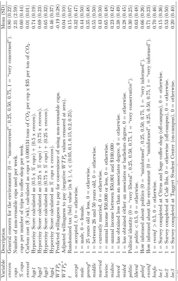
Definitions and summary statistics for variables used in our analysis are presented in Table 1. The
study’s two key variables are envcost and hyp[#]. Variable envcost represents an individual’s weekly
environmental cost associated with using non-reusable rather than reusable cups. The cost is calculated
as the product of (1) the number of non-reusable cups used per week (both cardboard and plastic), i.e.,
variable cups in Table 1, (2) the amount of embodied carbon per non-reusable cup (in pounds), and
(3) the per-pound equivalent carbon price. In turn, the number of non-reusable cups used per week
is self-reported by the survey respondent. Embodied carbon dioxide (CO2) per cup is estimated to be
0.25 pounds (Alliance for Environmental Innovation, 2000; Carbonrally.com, 2012), and the per-pound
equivalent price of $35 per ton represents the expected average carbon price through the year 2020 (Point
Carbon, 2010).16 Thus, for example, an individual who uses five non-reusable cups per week is estimated
to produce the equivalent of roughly $0.02 in weekly environmental costs associated with the carbon
14Logan is Cache County’s largest city, located in the northeast corner of Utah (see red highlighted areas in Figures 1 and
2). In 2009, Logan’s population consisted of 46,000 people residing in 16,000 households (U.S. Census Bureau, 2010). At the time of the survey, each of the four coffee shops provided small discounts for use of reusable cups. The average discount was 10 cents per cup (none of the shops allowed for free refills). Therefore, to the extent that the reusable-cup discounts may be biasing our hypocrisy scores and WTP-for-convenience estimates relative to coffee drinkers located outside of the study area who frequent shops that do not offer discounts, the bias is downward.
15
This estimate is based on pretests conducted with friends and colleagues, as well as informal feedback from actual survey participants.
16
The Alliance for Environmental Innovation and carbonrally.com report an estimate of embodiedCO2solely for cardboard
emitted through the life-cycle of the cups. The $0.02 cost estimate is calculated as follows: (5 cups) x
(0.000134 tons of CO2 per cup) x ($35 per ton of CO2) = $0.02, where the 0.000134 tons of CO2 per
cup is determined according to the relation 0.25 lbs. = 0.000134 tons. As Table 1 indicates, the average
coffee drinker in our sample contributes $0.01 of CO2 damage to the environment per week.
INSERT TABLE 1 HERE
As alluded to in Section 1, variable hyp[#] is calculated as a convex combination of variablesenvcon
and % cups, where envcon represents the “professing standards, beliefs, etc.” portion of hypocrisy’s
definition and% cups represents the “actual behavior” portion.17 An appealing aspect of the individual’s
coffee-cup choice is the relative ease with which it lends itself to a test of hypocritical behavior in strict
accordance with hypocrisy’s definition. The definition is unconcerned with what might abet a person’s
hypocrisy, i.e., it does not confuse or excuse hypocrisy as mere forgetfulness, laziness, or ignorance.
Nor does the definition distinguish rational from irrational hypocrisy (as purely economic thinking is
predisposed to do).18 Thus, the fundamental meaning of the definition can be captured in a single variable
such as hyp[#], which, although somewhat opaque in its intra-personal interpretation, does permit a
rather clear interpersonal comparison, i.e., an individual with a higher hyp[#] is indeed behaving more
hypocritically.
Still, hypocrisy’s definition gives no hint about which of its portions – profession of standards, beliefs,
etc., or actual behavior – is more important, which in turn creates the need for examining various weighting
schemes.19 In this study, variablehyp1 gives equal weight toenvconand% cups, whilehyp2 andhyp3 give
relatively more(less) weight toenvcon, respectively.20 Regardless of the weighting scheme, the minimum
and maximum values of hyp[#] are zero and one, respectively. As Table 1 indicates, the average coffee
drinker in our sample exhibits hypocritical behavior at the rates of 74%, 69%, and 65%, respectively,
based on the definitions ofhyp1,hyp2, and hyp3.
17As question 12 of the survey indicates, envcon is based on a five-point scale in response to a single, general question
about the individual’s self-perceived concern for the environment (see Appendix A). We purposefully eschewed using Dunlap et al.’s (2000) New Ecological Paradigm (NEP) scale to gauge each individual’s level of environmental concern because of the anticipated time it would take to complete the series of 15 questions necessary to create the scale. The NEP is better suited to an online survey format, where the typical respondent would have more time to complete the survey. We also worded the
envcon question as generally as possible in order to reduce the potential for a respondent to bias their answers to other key survey questions. For example, if ourenvcon question had asked respondents about their concerns regarding excessive use of disposable material and the resulting pressure such usage puts on landfill space – rather than just about their concern for the environment in general – it is more likely that at least some of the respondents would have felt pressure to bias their answers to the questions forcups and% cupsin order not to appear hypocritical.
18
Hypocrisy is also not to be confused with the gap between intention and action, or with boldfaced lying, as encountered by Davies et al. (2002).
19
Note that there is no theoretical basis upon which to formulate a quantitative measure of hypocrisy, only the admittedly loose guidance provided by its definition.
20
A potential problem with our hypocrisy score occurs whenever comparisons are made across individuals
who have zero values for either % cups or envcon, respectively. This can be explained most lucidly by
way of example. Suppose we have two individuals: Individual A with a hypocrisy score of zero (i.e.,
envcon=% cups= 0), and IndividualB with a score larger than zero, say as a result of envcon= 0 and
% cups > 0. Intuitively, because envcon = 0 for both A and B, we have no basis to determine which
individual is behaving more hypocritically. Yet, hyp[#] scores B higher. Similarly for the case where B
has envcon>0 but % cups= 0. In Section 3, we test for whether this “zeros problem” is affecting our
empirical results.21
The zeros problem is, in some sense, a specific case of the more general “distinguishability problem”,
whereby two individuals with the same or very similar hypocrisy scores actually exhibit distinct forms of
hypocritical behavior. For example, in the case ofhyp1 (where envcon and % cups are weighted equally
in the score’s determination), Individuals A and B could each have scores of 0.75%, but with A’s score
based upon envcon = 0.5 and % cups = 1, and B’s score based upon envcon = 1 and % cups = 0.5.
Clearly, IndividualA’s hypocrisy stems more from her use of non-reusable cups than her concern for the
environment, and vice-versa for Individual B. In Section 3, we also test empirically for the existence of
this more general type of problem in our data.
Finally, a potential concern about the validity of our hypocrisy measure arises due to the possibility
of a predetermined relationship between hyp[#] and envcost. This concern hinges on the possibility of
confounding correlation between% cups, which is included linearly in the definition ofhyp[#], and cups,
which is included linearly in the definition ofenvcost – refer to Table 1 for the specific definitions of these
variables. Theoretically, there is no reason to believe that a positive relationship should necessarily exist
between these two variables. For example, consider Individual A, who visits a coffee shop only twice
per week and each time takes her coffee in a cardboard cup. Individual B, on the other hand, visits a
coffee shop six times per week and takes his coffee in a cardboard cup four of those times. Relatively
speaking, Individual A’s total number of cups is small (cups = 2), and her percentage of cups large
(% cups= 100), while Individual B’s total number of cups is large (cups= 4) and his percentage small
(% cups= 67). In this case, the relationship between cups and % cups is negative rather than positive.
A similar example can just as easily be constructed showing a positive rather than negative relationship.
In general, therefore, one might expect positive and negative relationships of this sort to offset, or at least
21
counterbalance one another to some degree in any given dataset.
To assess whether a potentially confounding relationship betweenhyp[#] andenvcost exists in our
par-ticular dataset, i.e., to assesshyp[#]’s statistical validity, we conduct both non-parametric and parametric
tests. For the non-parametric test, we calculate Pearson correlation coefficients for each explanatory
vari-able used in our regression analysis, which envari-ables us to assess the relative strength of hyp[#]’s linear
relationship with envcost.22 For the parametric test, we redefine hyp[#] as the product of % cups and
envcon (henceforth hyp4) and run the same regression with hyp4 as was done with hyp1 – hyp3. Any
quantitative or qualitative differences that exist between the two regressions point to potential validity
problems with hyp1 – hyp3. This is because hyp4 does not suffer from a potential zeros problem. It is
also less susceptible to statistical invalidity because the exact covariance betweenhyp4 – which, again, is
defined as the product of two random variables) andenvcost – is an exceedingly complicated collection of
expectation and covariance terms, as pointed out by Bohrnstedt and Goldberger (1969). As a result, one
cannot necessarily determine a priori, from their respective definitions alone, how these types of random
variables will correlate with one another given an actual dataset. Results for these non-parametric and
parametric tests are reported in Section 3.
Additional variables of interest in our regression analysis include W T Pp and politic. VariableW T Pp
is the individual’s predicted willingness-to-pay (W T P) for the convenience of using a non-reusable cup.
Convenience, in turn, is a catch-all for foibles such as forgetfulness and laziness, which might otherwise
confound our estimates of hypocrisy’s effects on environmental cost. Table 1 reports means for two
measures of W T Pp. The first, W T Pp = -$ 0.19 per non-reusable cup, is an empirically estimated mean
WTP based on an interval regression model (discussed in Section 3). The second, W T Pp∗ = $ 0.04 per
cup, results from having censored all negative W T Pp values at zero (roughly 72% of our sample of 521
observations). Variable W T Pp∗ accounts for the fact that paying individuals for the ‘inconvenience’ of
using a non-reusable cup (i.e., considering the possibility of negative WTP for use of a cardboard or
plastic cup) is unrealistic.23
The survey question used to create the variablepoliticwas included in the survey in order to deflect the
participant’s attention away from the environmental concern question (which was used to createenvcon).
The goal here was to preclude the participant from correctly guessing that the survey’s intent was to
22
Point biserial, rather than Pearson, correlation coefficients are calculated for all dummy variables used in the regression analyses in order to correct for the nominal vs. quantitative nature of these calculations.
23
measure hypocrisy. As an added bonus, politic controls for political viewpoint, similar to how W T Pp
controls for convenience. As indicated in Table 1, the average individual in our sample self-identifies
as having left-of-center political beliefs (which, based on Cache County’s historical voting record, is
unrepresentative of the county’s population at large).24
3
Empirical Model and Results
We estimate a simple ordinary least squares (OLS) model of hypocrisy’s effect on individual i’s carbon
cost,25
envcosti =Xiα+i (1)
whereXi represents a vector of explanatory variables including individuali’s demographic characteristics
a l´a survey questions 5 - 9, and self-perceptions a l´a survey questions 10 - 13 (see Appendix A). Also
included in vectorXi is the individual’s hypocrisy score and predicted willingness-to-pay for convenience.
Theα term represents a vector of corresponding (constant) coefficients to be estimated, andi is an i.i.d
error term.
The individual’s predicted willingness-to-pay,W T Pp, is derived from prior interval regression analysis
following Woolridge (2002). Accordingly, based on his response to a given bid value, ti, the individual’s
latent willingness-to-pay, W T Pl is placed in one of two regions: (-∞,ti) in the event of answering “no”
to the willingness-to-pay question, and (ti, ∞) in the event of answering “yes.”26 W T Pl for individual
i (in its reduced form, as a solution to a standard random-utility model) is assumed linear in both its
deterministic and random components,
W T Pli=Yiβ+µi (2)
where, similar to vectorXi,Yirepresents a vector of explanatory variables (which in this case includesti),
β represents a vector of corresponding (constant) coefficients to be estimated, andµi is a corresponding
i.i.d error term. For estimation purposes we define binary choice variable,accepti, as equaling one if the
respondent accepts ti and zero if not. Thus, accepti = 1 responses imply W T Pli > ti and accepti = 0
24
Our sample is, however, more representative of the city’s gender composition (44% male for our sample vs. 49% for Logan city) and income distribution (65% (23% ) low-(mid-) income for our sample vs. 69% (23.5% ) for Logan city) (U.S. Census Bureau, 2010).
25We use STATA IC/11.0 for Windows (64 bit). 26
implies W T Pli ≤ti (Caplan et al, 2010). Using equation (2), the probability that respondent i accepts
bidti is,
Pi =P r[accepti = 1] =P r[W T Pli> ti] =P r[µi> ti−Yiβ] = Φ (Yiβ−ti) (3)
where Φ (·) is a standard normal cumulative distribution function, with the last equality following from
Φ (·)’s symmetry. Using (3), the associated log likelihood function defined over all individualsi= 1, ..., N,
is,
LogL=
N
X
i=1
[accepti(ln(Pi)) + (1−accepti) (ln(1−Pi))] (4)
where,LogLis estimated using an interval regression model (Woolridge, 2002). Results for the estimation
of equation (4) are provided in Appendix B.
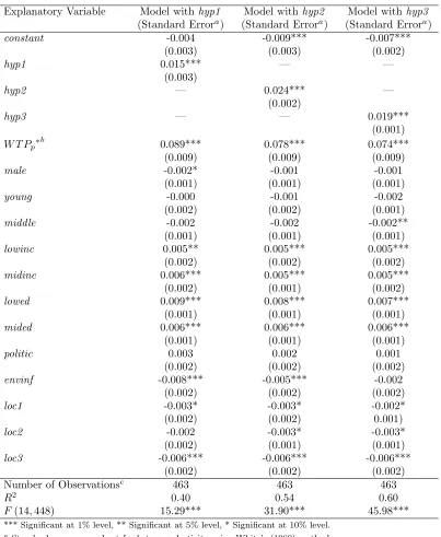
Table 2 presents our results for the estimation of equation (1). Of primary interest is the set of
coefficient estimates forhyp1 – hyp3, each of which is positive and statistically significant at the 1% level
of significance. For example, the coefficient estimate for hyp2 indicates that as the average individual’s
hypocrisy score increases by one percent he contributes roughly $0.0002 in additional global carbon costs,
all else equal.27 To put this result in context, if the average coffee drinker in our sample reduces his
hypocrisy score (in this case hyp2), by one percent (from 0.69 to 0.68, see Table 1), then, using the
formula forenvcost in Table 1, this change is estimated to result in a reduction of roughly (5/100)ths of a
non-reusable cup per week ((0.01 reduction inhyp2 x 0.024)/(0.000134 tons ofCO2 per cup x $35 per ton
ofCO2), where 0.024 is the coefficient estimate forhyp2 from Table 2), all else equal. Thus, inducing the
average coffee drinker to completely eliminate his use of 2.31 non-reusable cups per week would require a
reduction in his hypocrisy score of roughly 0.46 (i.e., from 0.69 down to 0.23).
INSERT TABLE 2 HERE
The usual caveat applies with respect to what might motivate the coffee drinker to reduce his hypocrisy
score in the first place, and how he generates the reduction. All we are permitted to say in this study
is that, all else equal, our data suggests a relatively large reduction in his hypocrisy score is required to
27It is important to note that this regression result, i.e., the positive relationship between hyp2 and envcost, is not
predetermined by hyp2’s definition. This is because, in general, coefficient estimates reflect the covariance between the respective dependent and independent variables that exist in the data at hand, not the partial derivatives of the definition of the dependent variable per se. In our case, the calculation ofenvcost, which is simply the variablecups scaled by a common constant term across all observations, does not admit collinearity withhyp2, which is calculated as a convex combination of the variables% cupsandenvcon – see Table 1. First,% cupsandcups are not per force perfectly collinear (in our case the Pearson correlation coefficient between these two variables is 0.65). Second, the fact that% cupsis effectively multiplied by
envconin the definition ofhyp2, andenvconis not per force collinear withcups, collinearity is again absent betweenenvcost
induce the average coffee drinker to eliminate his dependence on non-reusable cups. We do not attempt
in this study to identify why or how this reduction in hypocrisy comes about. With respect to “why”,
the reduction may be a consequence of value formation (e.g., Hoehn and Randall, 1987) or preference
learning (e.g., Crocker and Shogren, 1991), either of which seems plausible. With respect to “how” his
hypocrisy score is reduced, we know only that the average individual’s reduction does not come about
strictly through a decrease in his envcon value (i.e., the “professing standards, beliefs, etc.” portion of
hypocrisy’s definition). If this were the case, then on average no concomitant change would occur in
envcost. Thus, all we can say is that what would ultimately drive the average individual to reduce his
hypocrisy score is either purely a reduction in his % cups value (i.e., the revealed-preference portion of
hypocrisy’s definition) or, most likely, some combination of reductions in hisenvcon and % cups values.
As indicated in Table 2, a positive contribution to carbon cost is also linked to the need for convenience
(the marginal effect of a one-cent increase in an individual’sW T Pp∗ is roughly $0.0009 in weekly carbon
costs), suggesting that a coffee drinker’s hypocritical behavior and need for convenience do indeed take
an environmental toll. Similar tolls on the environment can be attributed to an individual’s (1) being
relatively uninformed about environmental issues, (2) being female, (3) being low or middle income, and
(3) not having attained a relatively high education level.28 These marginal effects are, for the most part,
robust across the three models (except, perhaps, with respect to being female). Further, the F and R2
statistics for each model indicate relatively good overall statistical fits of the data, with roughly half of
the total variation inenvcost explained by the models’ respective covariates.
As mentioned in Section 2, a potential “zeros problem” exists with respect to hyp1 – hyp3, which
could be affecting the results reported in Table 2. To test for the presence of this problem in our data,
we first dropped from the sample all observations associated with% cups= 0 (111 observations dropped)
and re-estimated equation (1) for hyp1,hyp2, andhyp3, respectively. We then dropped from the sample
all observations associated withenvcon= 0 (four observations dropped) and again re-estimated equation
(1) for hyp1, hyp2, and hyp3, respectively. In all cases, the results were qualitatively the same as those
in reported in Table 2, suggesting that the zeros problem is not present in our data. Similarly, to test
for the presence of a “distinguishability problem” in the data, we sequentially dropped observations with
envcon= 0 (four observations dropped), envcon≤0.25 (22 observations dropped), and envcon≤0.5 (69
observations dropped), and then re-estimated equation (1) for hyp1,hyp2, andhyp3. In other words, we
28
successively eliminated those individuals whose hypocrisy stems more and more from their concern for
the environment (thus eliminating the basis for a distinguishability problem at the outset). As with the
absence of a zeros problem in our data, in all cases the results were qualitatively the same as those in
reported in Table 2, suggesting that the distinguishability problem is also not present in our data.29
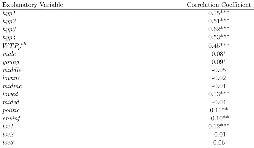
As mentioned in Section 2, an additional, potential concern about the validity of our hypocrisy measure
arises due to the possibility of a predetermined relationship between hyp1 – hyp3 and envcost.
Non-parametric, Pearson correlation coefficients are reported in Table 3 (point biserial correlation coefficients
are reported for the dummy variables, which include all variables excepthyp1 –hyp4 andW T Pp∗). These
coefficients are estimates of the linear relationship between the given explanatory variable and envcost.
Among the set of explanatory variables included in Table 2, the hyp3,hyp4, andhyp2 variables have the
strongest correlations with envcost, followed by W T Pp∗,hyp1, and lowed. Variables politic, envinf, loc1,
male and young also exhibit statistically significant correlations withenvcost.
INSERT TABLE 3 HERE
These results, which prima facie draw into question the statistical validity of hyp3, need to be
com-pared with the regression results reported in Table 2. In particular, several of the variables that are
statistically significant regressors in Table 2 obtain insignificant correlation coefficients in Table 3, and
vice-versa. For example, lowinc,midinc,mided,loc2, andloc3 all have statistically significant regression
coefficients, but insignificant correlation coefficients. Variables young and politic have statistically
in-significant regression coefficients, but in-significant correlation coefficients, andloc1’s correlation coefficient
obtains a noticeably lower level of significance than its regression coefficient. Correlation coefficients,
therefore, do not necessarily distinguish the statistical validity of hyp1 –hyp3.
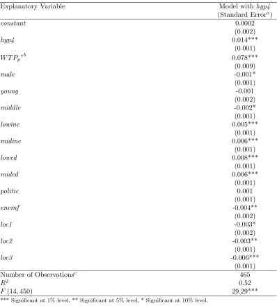
In our case, a better indication of hyp1’s – hyp3’s statistical validity is obtained via the parametric
results presented in Table 4. Here, as described in Section 2, hyp4, which by design is less susceptible to
statistical invalidity, is regressed against the same set of explanatory variables as in Table 2. As indicated,
the results are striking in both their qualitative and quantitative similarities with those reported in Table
29We also tested for the presence of a distinguishability problem by sequentially eliminating those individuals whose
2. Based upon these results, we feel confident in concluding that confounding relationships between our
original measures of hypocrisy (hyp1 – hyp3) and envcost do not exist.
INSERT TABLE 4 HERE
Lastly, Table 5 presents results for the interaction of our demographic variables with hyp1,hyp2, and
hyp3, respectively. For ease of interpreting the interactive effects of political identity and the perception
of being informed about environmental issues, we have created two new dummy variables. Variableliberal
equals one if the individual’s corresponding value for politic is less than 0.5, i.e., the individual rates
himself “left-of-center” on the political scale, and zero otherwise. Similarly, variable hinfo equals one
if the individual’s corresponding value for envinf is greater than 0.5, i.e., the individual rates himself
“higher-than-middle” on the environmentally-informed scale, and zero otherwise.
INSERT TABLE 5 HERE
As the table indicates, with respect to hyp1 the hypocrisy effect is larger for younger, male,
lower-educated, more-conservative, and less-environmentally informed individuals. However, the larger effect
only holds for lower-educated, more-conservative males when considering hyp2, and only for males when
considering hyp3. These results suggest that different types of coffee-drinking hypocrites affect the
envi-ronment to varying extents.
4
Summary and Conclusions
As this study suggests, economists likely have something to add to the musings of philosophers and
psychologists on the subject of hypocrisy. That “something” is a quantitative assessment of hypocrisy’s
environmental costs. In studying the choices coffee drinkers make with respect to the type of cup in which
their drink is taken – reusable vs. non-reusable – we find that each percentage increase in an individual’s
“hypocrisy score” results in roughly $0.0002 in additional costs associated with carbon emissions per
week. This hypocrisy effect is larger for younger, male, lower-educated, more-conservative, and
lesser-environmentally informed coffee drinkers when equal weight is assigned to the ‘actual behavior’ and
‘professed standards’ components of their hypocrisy scores.
Although the magnitude of the estimated cost associated with this human foible is admittedly small
for coffee drinkers, the problem of hypocrisy merits attention. Our empirical results suggest that the
To see this, note from Table 1 that the average drinker adds roughly $0.01 per week in global carbon costs
due to his use of non-reusable cups. We estimate the (private) benefit obtained from using non-reusable
cups (in the form ofW T P for their convenience) to be as low as -$0.19 and as high as $0.04 per cup. To
the extent that hisW T P for convenience is therefore less than $0.01 on a weekly basis, a net social gain
from reducing the typical drinker’s use of non-reusable cups is indeed attainable. Although our coefficient
estimates forhyp[#] in Table 2 suggest that, all else equal, a relatively large reduction in a coffee drinker’s
hypocrisy score is needed to induce the requisite reduction in carbon cost (recall our discussion in Section
3), there appears to be plenty of scope for such a reduction, as the average drinker scores in a range of
65% to 74% on the hypocrisy scale (Table 1).
The question naturally arises, why attempt to reduce people’s hypocrisy through “deep regulation”,
e.g., through a cognitive-dissonance campaign geared toward instilling guilt and introspection, when
taxation, subsidization, or the provision of technical information could potentially serve the same purpose
(perhaps at a relatively lower cost per cup)?30 Our answer is twofold. First, creating cognitive dissonance
in an individual’s mind – specifically via pointing out an individual’s hypocrisy – has been shown to induce
behavioral changes in a variety of contexts (see for instance, Stone et al., 1994; Fointiat, 2004; and Son
Hing et al., 2002).31 Second, the possible spillover effects associated with confronting people about their
hypocritical choices in life likely outweigh those that would be obtained through standard price incentives,
particularly when the cognitive-dissonance campaign is coupled with provision of information targeting
a specific environmental problem – in our case the carbon cost associated with the use of non-reusable
coffee cups.
Similar to how rational behavior induced in market settings can spillover to non-market valuation
settings (Cherry et al., 2003), pointing out hypocrisy in one market setting may encourage less hypocritical
behavior in other market settings. Granted, wrestling with one’s hypocrisy when it comes to choosing
which type of cup to take coffee or tea in is one thing. When it comes to making other choices that have far
greater environmental impacts, such as which mode of transportation to choose for day-to-day travel, or
where and how to travel for vacation, the payoffs associated with reducing one’s corresponding hypocrisy
scores may be far more profound. Through deeper introspection, of the kind Rochefoucauld, Heschel, and
Jung surely strove to provoke in us, we would be taking personal ownership of the externalities to which
30Festinger (1957) is generally credited with coining the term “cognitive dissonance”, which is an aversive state of
psy-chological tension aroused when an individual two inconsistent cognitions (Rubens et al., 2013). According to Rubens et al. (2013), Festinger (1957) believed that people are motivated to reduce this dissonance by changing one or both of the inconsistent cognitions.
31Rubens et al. (2013) find that these behavioral changes are not robust to delays between pointing out the individual’s
we contribute, perhaps with a longer-lasting effect on our consumptive behaviors.
As mentioned in Section 1, this study’s results also have an important methodological implication. The
long-held presumption among stated-preference researchers that (in well-designed surveys) hypothetical
bias alone distinguishes revealed from stated values or behavior is incorrect. Part of this difference could
in fact be explained by an individual’s hypocritical behavior. Controlling for hypocritical bias would
therefore refine our measurements of the bias we heretofore have attributed solely to the hypothetical
References
Aadland, D. and A.J. Caplan (2006) “Curbside Recycling: Waste Resource or Waste of Resources?”
Journal of Policy Analysis and Management 25(4), 855-874.
Ajzen, I, T.C. Brown, F. Carvajal (2004) “Explaining the Discrepency Between Intentions and Actions:
The Case of Hypothetical Bias in Contingent Valuation.” Personality and Social Psychology Bulletin
30(9), 1108-1121.
Alliance for Environmental Innovation (2000) Report of the Starbucks Coffee Company/Alliance
for Environmental Innovation Joint Task Force. A Project of Environmental Defense
and The Pew Charitable Trusts. Retrieved from the internet on January 28, 2012 at
http://business.edf.org/sites/business.edf.org/files/starbucks-report-april2000.pdf.
Andreoni, J. (1995) “Warm-Glow Versus Cold-Prickle: The Effects of Positive and Negative Framing on
Cooperation in Experiments.” The Quarterly Journal of Economics 110(1), 1-21.
Bohrnstedt, G.W. and A.S. Goldberger (1969) “On the Exact Covariance of Products of Random
Vari-ables.” Journal of the American Statistical Association 64(328), 1439-1442.
Caplan, A. J., Jackson-Smith, D., and Marquart-Pyatt, S. (2010) “Does ‘Free Sampling’ Enhance the
Value of Public Goods?” Applied Economics Letters 17(4), 335-339.
Carbonrally.com (2012) De-Cup Your Decaf. Retrieved from the internet on January 30, 2012 at
http://www.carbonrally.com/challenges/12-paper-coffee-cups/.
Champ, P.A., Bishop, R.C., Brown, T.C., and MCCollum, D.W. (1997) “Using Donation Mechanisms
to Value Nonuse Benefits from Public Goods.” Journal of Environmental Economics and Management
33, 151-162.
Cherry, T. L., Crocker, T. D., Shogren, J. F. (2003) ”Rationality Spillovers.” Journal of Environmental
Economics and Management 45, 63-84.
Collins English Dictionary (2003) New York: HarperCollins Publishers. Retrieved from the internet on
Crocker, T., and J.F. Shogren (1991) “Preference Learning and Contingent Valuation Methods.”
Environ-mental Policy and the Economy. F. Dietz, F.Van der Ploeg, and J.Van der Straaten, eds., Amsterdam:
North-Holland Publishers.
Cummings, R.G., S. Elliot, G.W. Harrison, and J. Murphy (1997) “Are Hypothetical Referenda Incentive
Compatible?” Journal of Political Economy 105, 609-621.
Davies, J. Foxall, G.R., and Pallister, J. (2002) “Beyond the Intention-Behavior Mythology: An Integrated
Model of Recycling.” Marketing Theory 2, 29-113.
Dunlap, R., Van Liere, K., Mertig, A., and Jones, R.E. (2000) “Measuring Endorsement of the New
Ecological Paradigm: A Revixed NEP Scale.” Journal of Social Issues 56, 425-442.
Festinger, L. (1957)A Theory of Cognitive Dissonance. Oxford, UK: Row, Peterson.
Fointiat, V. (2004) “I Know What I have to Do, But: When Hypocrisy Leads to Behavioral Change.”
Social Behavior and Personality 32, 741-746.
Fox, J.A, Shogren, J.F., Hayes, D.J., and Kliebenstein, J.B. (1998) “CVM-X: Calibrating Contingent
Values with Experimental Auction Markets.” American Journal of Agricultural Economics 80,
455-465.
Greene, W.H. (2011) Econometric Analysis. New York: Pearson College Division.
Heschel, A.B. (1955) God in Search of Man: A Philosophy of Judiasm. New York: Farrar, Straus, and
Giroux.
Hoehn, J. and A. Randall (1987) “A Satisfactory Benefit Cost Indicator from Contingent Valuation.”
Journal of Environmental Economics and Management 14, 226-247.
International Coffee Organization (ICO) (2013) “ Coffee Facts.” Retrieved from the internet on July 3,
2013 at http://www.ico.org/show-faq.asp?show=35.
Jung, C.G. (1966) Two Essays on Analytical Psychology, Collected Works, Volume 7. Princeton, N.J.:
Princeton University Press.
Krinsky, I. and Robb, A. (1986) “Approximating the Statistical Properties of Elasticities.” Review of
LaPiere, R.T. (1934) “Attitudes vs. Actions.” Social Forces 13, 230-237.
Loomis, J., Brown, T.C., Lucero, B., and Peterson, G.L. (1996) ”Improving Validity Experiments of
Contingent Valuation Methods: Results of Efforts to Reduce the Disparity of Hypothetical and Actual
WTP.” Land Economics 72, 450-461.
Mazar, N. and C-B Zhong (2010) “Do Green Products Make Us Better People?” Psychological Science
20(5), 1-5.
Mitchell, R.C., and R.T. Carson (1989)Using Surveys to Value Public Goods: The Contingent Valuation
Method. Washington, DC: Resources for the Future.
Point Carbon (2010)Carbon 2010: return of the sovereign. Report published at Point Carbons 6th annual
conference, Carbon Market Insights 2010 in Amsterdam, March 2 – 4. Retrieved from the internet on
January 30, 2012 at http://www.pointcarbon.com/polopoly fs/1.1545246Carbon202010.pdf.
Rochefoucauld, F. de La (1665-1678) Reflections; or Sentences and Moral Maxims, Maxim 218.
Rubens, L., Gosling, P., Bonaiuto, M., Brisbois, X., and Moch, A. (2013) “Being a Hypocrit or Committed
While I Am Shopping? A Comparison of the Impact of Two Interventions on Environmentally Friendly
Behavior.” Environment and Behavior 20(10), 1-14.
Son Hing, L.S., Li, W., and Zanna, M.P. (2002) “Inducing Hypocrisy to Reduce Prejudicial Responses
Among Aversive Racists.” Journal of Experimental Social Psychology 38, 71-78.
Stone, J., Aronson, E., Crain, A.L., Winslow, M.P., and Fried, C.B. (1994) “Inducing Hypocrisy as a
Means of Encouraging Young Adults to Use Condoms.”Personality and Social Psychology Bulletin 20,
116-128.
U.S. Census Bureau (2010)American Fact Finder. Retrieved from the internet on December 17, 2011 at
http:// factfinder2.census.gov.
White, H. (1980) “A Heteroskedasticity-Consistent Covariance Matrix Estimator and a Direct Test for
Heteroskedasticity.” Econometrica 48, 817-838.
Woolridge, J.M. (2002) Econometric Analysis of Cross Section and Panel Data. The MIT Press:
Table 2: Regression Results for envcost.
Explanatory Variable Model withhyp1 Model withhyp2 Model withhyp3
(Standard Errora) (Standard Errora) (Standard Errora)
constant -0.004 -0.009*** -0.007***
(0.003) (0.003) (0.002)
hyp1 0.015*** — —
(0.003)
hyp2 — 0.024*** —
(0.002)
hyp3 — — 0.019***
(0.001)
W T Pp∗ b
0.089*** 0.078*** 0.074***
(0.009) (0.009) (0.009)
male -0.002* -0.001 -0.001
(0.001) (0.001) (0.001)
young -0.000 -0.001 -0.002
(0.002) (0.002) (0.001)
middle -0.002 -0.002 -0.002**
(0.001) (0.001) (0.001)
lowinc 0.005** 0.005*** 0.005***
(0.002) (0.002) (0.002)
midinc 0.006*** 0.005*** 0.005***
(0.002) (0.001) (0.002)
lowed 0.009*** 0.008*** 0.007***
(0.001) (0.001) (0.001)
mided 0.006*** 0.006*** 0.006***
(0.001) (0.001) (0.001)
politic 0.003 0.002 0.001
(0.002) (0.002) (0.002)
envinf -0.008*** -0.005*** -0.002
(0.002) (0.002) (0.002)
loc1 -0.003* -0.003* -0.002*
(0.002) (0.002) 0.001)
loc2 -0.002 -0.003* -0.003*
(0.002) (0.001) (0.001)
loc3 -0.006*** -0.006*** -0.006***
(0.002) (0.002) (0.002)
Number of Observationsc 463 463 463
R2 0.40 0.54 0.60
F(14,448) 15.29*** 31.90*** 45.98***
*** Significant at 1% level, ** Significant at 5% level, * Significant at 10% level.
aStandard errors are robust for heteroscedasticity using White’s (1980) method.
bStandard errors are bootstrapped (5000 replications).
Table 3: Correlation Coefficients (Between envcost and Explanatory Variables).
Explanatory Variable Correlation Coefficient
hyp1 0.15***
hyp2 0.51***
hyp3 0.62***
hyp4 0.53***
W T Pp∗b 0.45***
male 0.08*
young 0.09*
middle -0.05
lowinc -0.02
midinc -0.01
lowed 0.13***
mided -0.04
politic 0.11**
envinf -0.10**
loc1 0.12***
loc2 -0.01
loc3 0.06
Table 4: Regression Results forenvcost Withhyp4.
Explanatory Variable Model withhyp4
(Standard Errora)
constant 0.0002
(0.002)
hyp4 0.014***
(0.001)
W T Pp∗ b
0.078*** (0.009)
male -0.001*
(0.001)
young -0.001
(0.002)
middle -0.002*
(0.001)
lowinc 0.005***
(0.001)
midinc 0.006***
(0.001)
lowed 0.008***
(0.001)
mided 0.006***
(0.001)
politic 0.001
(0.001)
envinf -0.004**
(0.002)
loc1 -0.003*
(0.002)
loc2 -0.003**
(0.001)
loc3 -0.006***
(0.001)
Number of Observationsc 465
R2 0.52
F(14,450) 29.29***
*** Significant at 1% level, ** Significant at 5% level, * Significant at 10% level.
aStandard errors are robust for heteroscedasticity using White’s (1980) method.
bStandard errors are bootstrapped (5000 replications).
Table 5: Regression Results for Interaction Terms.a
Interaction Term Interacted withhyp1 Interacted withhyp2 Interacted withhyp3
(Standard Errorb) (Standard Errorb) (Standard Errorb)
male 0.002* 0.003** 0.004**
(0.001) (0.001) (0.002)
young 0.003* 0.001 0.000
(0.001) (0.001) (0.002)
middle -0.002 -0.001 -0.000
(0.001) (0.001) (0.001)
lowinc -0.000 0.000 -0.000
(0.001) (0.001) (0.002)
midinc -0.001 -0.001 -0.001
(0.002) (0.002) (0.002)
lowed 0.004*** 0.003** 0.002
(0.001) (0.001) (0.001)
mided -0.001 -0.000 -0.000
(0.002) (0.002) (0.002)
liberal -0.003*** -0.003* -0.002
(0.001) (0.001) (0.002)
hinfo -0.004*** -0.002 0.001
(0.001) (0.001) (0.001)
*** Significant at 1% level, ** Significant at 5% level, * Significant at 10% level.
aSeparate regressions were run for each interaction term, which included only a constant
andhyp[#], along with the interaction term itself.
Figure 1: Location of Utah.
Appendix A: The Coffee Shop Survey
Thank you for agreeing to complete this survey. Your responses will help inform research being conducted
by [NAMES REMOVED FOR SAKE OF ANONYMITY]. Once you have completed the survey, please fold
it and slip it into the cardboard box marked “coffee shop survey” located near the cash register. The USU
Institutional Review Board for the protection of human participants (IRB) has approved this study. If you
have any questions or concerns you may contact [NAME REMOVED FOR SAKE OF ANONYMITY] at
[NUMBER REMOVED FOR SAKE OF ANONYMITY] or email [ADDRESS REMOVED FOR SAKE
OF ANONYMITY]. If you would like to contact someone other than the research team, you may contact
the IRB Administrator at (435) 797-0567 or email [email protected].
1. On average, approximately how many times per week do you visit a coffee shop to get a cup of coffee
or tea?
times per week.
2. On average, approximately what percentage of the time during a typical week do you take your coffee
or tea in a cardboard cup or plastic cup provided by the coffee shop(s)? (Please provide answers for both
Cardboard Cup and Plastic Cup).
Cardboard Cup % Plastic Cup %
If you answered anything greater than 0% to Cardboard Cup or Plastic Cup in Question
2, please answer the next two questions (Questions 3 and 4). Otherwise, you can skip to
Question 5.
3. Before you answer this question, please think about 1) your income level, 2) your monthly expenses,
and 3) how many times you visit a coffee shop during an average week. If the coffee shop(s) you visit on
a regular basis begin charging you an extra $xx per cardboard cup and per plastic cup, would you switch
to using a reusable cup for every visit to the coffee shop(s)? (By “reusable cup” we mean any metal or
plastic container that you bring with you to the coffee shop, or ceramic cup provided by the coffee shop,
that can be reused multiple times, year after year.)
Yes, I would switch to using a reusable cup for each trip to the coffee shop.
No, I would not switch to using a reusable cup for each trip to the coffee shop.
If you answered “Unsure” to Question 3, please skip to Question 5. Otherwise, answer
Question 4 first.
4. Using the scale (1,2,3,4,5), with 1 meaning completely “uncertain” up to 5 meaning completely “certain”
how certain are you of your answer to the previous question (Question 3)?
5. What is your gender? Male Female
6. What is your age? years.
7. What is your current marital status?
Single
Living as domestic partners
Married
Divorced
Widowed
8. What is your approximate average annual income from both earned (i.e., your salary) and unearned
(i.e., mom and dad, inheritance, etc.) sources? (Please check one category.)
Less than or equal to $25,000 per year.
$25,001 - $50,000 per year.
$50,001 - $75,000 per year.
$75,001 - $100,000 per year.
$100,001 - $150,000 per year.
Greater than $150,000 per year.
9. What is the highest level of education you have completed at this point in time? (Please check one
category.)
0 - 8 years, no high school diploma or GED
9 - 12 years, no high school diploma or GED
High school diploma or GED
Some college, no degree yet obtained
Associates degree
Masters degree
Doctorate or professional degree
10. Using the scale (1,2,3,4,5), with 1 meaning “very liberal” to 5 meaning “very conservative,” how
would you rate your political views?
11. Using the scale (1,2,3,4,5), with 1 meaning completely “uninformed” to 5 meaning “very informed,”
how would you rate the degree to which you are informed about political issues in general?
12. Using the scale (1,2,3,4,5), with 1 meaning completely “unconcerned” to 5 meaning “very concerned,”
how would you rate your concern for the environment in general?
13. Using the scale (1,2,3,4,5), with 1 meaning completely “uninformed” to 5 meaning “very informed,”
how would you rate the degree to which you are informed about environmental issues in general?
The End. Thanks again for completing this survey. You may now put it in the cardboard box near the
cash register. If you borrowed one of our little pencils, we would appreciate it if you would also return it
Appendix B: Empirical Results for Willingness to Pay
Explanatory Variable Regression Coefficients Marginal Effects (Standard Error) (Standard Error)
constant -0.079 —
(0.394)
ti -1.656* -0.571*
(0.993) (0.342)
cups 0.065** 0.022**
(0.028) (0.009)
male 0.225 0.078
(0.149) (0.052)
young 0.053 0.018
(0.293) (0.102)
middle 0.183 0.063
(0.244) (0.083)
lowinc -0.346 -0.122
(0.239) (0.086)
midinc -0.312 -0.102
(0.245) (0.076)
lowed -0.415* -0.139*
(0.214) (0.069)
mided -0.212 -0.071
(0.205) (0.067)
loc1 -0.735** -0.212**
(0.312) (0.070)
loc2 -0.047 -0.016
(0.228) (0.079)
loc3 0.256 0.092
(0.253) (0.093)
Mean WTPa -0.19 (-2.12, 2.03) Adjusted Mean WTPb -0.25 (-2.41, 1.87)
Log likelihood -200.48
χ2(LR) 41.68***
PseudoR2 0.09
Number of Observationsc 355
Ω1=Predicted accept =1
Observed accept=1 0.04 Ω2=Predicted acceptObserved accept=0
=0 0.99
*** Significant at 1% level, ** Significant at 5% level, * Significant at 10% level.
aKrinsky and Robb (1986) 95% confidence interval in parentheses.
bAdjusted according to Champ et al.’s (1997) recoding method.
Appendix C: The Social Net Benefit of Eliminating Hypocrisy
Letui =ui(ai, ei;βi, γi) represent individuali’s continuously differentiable, quasi-concave utility function,
where (1) ai = (ai1, ..., aiJ) is i’s vector of activity levels for activities j= 1, ..., J, (2)ei is i’s perception
of the environment’s overall health, and (3) associated vector βi and scalar γi parameterize ui with
respect to ai and ei, respectively, such that ∂ui(·)/∂aij > 0,∀aij, and ∂ui(·)/∂ei > 0. Further, let
ei = fi(ai;a−i,θi,θ−i) represent the mapping function for i’s activity levels to his perception of the
environment’s health, where associated vector θi and matrixθ−i parameterize fi with respect to ai and
a−i, respectively, and subscript −i denotes all individuals other than individuali.32 For future reference
we assumeθi ensures∂fi(·)/∂aij <0,∀aij, i.e., each of the individual’s activities harms the environment.
If the individual behaves as ifθi =θiT has been inserted inf(·), whereθiT = θi1T, ..., θiJT
represents
i’s ‘professed’ parameter vector, then i exhibits no hypocrisy. In this case, individual i parameterizes
his environmental mapping function (and thus the perceived environmental-health portion of his utility
function) strictly according to his professed beliefs, and then behaves accordingly in choosing his activity
levels to maximize his welfare. It naturally follows that the number of θij parameters not set equal
to their corresponding θijT values defines the individual’s degree of hypocrisy. For example, insertion
of vector θi = θi16=θi1T, θi2T, ..., θiJT
denotes individual i as a first-degree hypocrite, insertion of
θi = θi1 6=θi1T, θi1 6=θi2T, θi3T, ..., θiJT
denotes second-degree hypocrisy, and so on. We assume that
fi(ai,a−i;θi,θ−i)> fi ai,a−i;θiT,θ−i
,∀θi 6=θiT, i.e., the perceived environmental effect of hypocrisy
is always negative in the sense that by not parameterizing his environmental mapping function strictly
according to his professed beliefs, the individual perceives his contribution to environmental damage (or,
reduced environmental health) as being less than it actually is.
Without loss of generality (for the purpose at hand) consider the simple case of quasi-linear preferences
defined over single-valued ai and a−i (e.g., taking coffee in a cardboard cup), and thus for single-valued
parametersβi,θi, andθ−i.33 Let the numeraire be defined asyi.34 Given local non-satiation of preferences,
the individual’s budget constraint holds with strict equality, i.e.,wi=yi+pai, wherewi isi’s wealth level
and p is the (given) per-unit cost of activityai. Individual i’s corresponding indirect utility can then be
32
We acknowledge that a personal information set also determines i’s perception of his contribution to environmental damage, but, for ease of exposition, do not explicitly include it as an additional parameter inf(·).
33
Recall thateiand associated parameterγiare single-valued by definition.
34For example, we can think ofi’s utility function looking something likeu
i(·) =yi+gi(ai, ei(·) ;a−i), where function
defined for the cases ofθi =θiT and θi6=θiT, respectively, as,
viT =vi p, wi, βi, γi, θiT, θ−i, a−i
(5)
˜
vi =vi(p, wi, βi, γi, θi, θ−i, a−i). (6)
where, given the earlier assumptions ∂fi(·)/∂aij <0,∀aij, and fi(ai,a−i;θi,θ−i)> fi ai,a−i;θiT,θ−i
,
∀θi 6= θiT, we know that in a Nash equilibrium (where individual i takes a−i as given), (1) ˜vi > viT,
(2) ˜ai > aiT, and (3) ˜ei > eiT, where (˜ai,˜ei) and aiT, eiT
are the optimal activity and perceived
environmental-health values associated with ˜vi and viT, respectively. In other words, in the process of
eliminating his hypocrisy individuali both reduces his activity leveland perceives environmental health
to be worse, which in turn reduces his maximum utility level.
Inverting equation (6) to obtain its associated expenditure function, ˜mi, and using the result ˜vi> viT,
leads to,
wi= ˜mi=mi(p, βi, γi, θi, θ−i, a−i,v˜i)> mi p, βi, γi, θi, θ−i, a−i, viT
. (7)
Willingness to pay to avoid having to correct for one’s hypocrisy, W T PiH, is then defined as,
W T PiH =wi−mi p, βi, γi, θi, θ−i, a−i, viT
>0. (8)
W T PiH is a measure of the cost individual i incurs (i.e., the welfare individual i loses) as a result of
eliminating his hypocrisy. This measure has been approximated (on a weekly basis) by W T Pp and
W T Pp∗ in our study. The corresponding (social) benefit has been approximated byenvcost. Thus, social