Influences of observation errors in eddy flux data on inverse model parameter estimation

www.biogeosciences.net/5/1311/2008/

© Author(s) 2008. This work is distributed under the Creative Commons Attribution 3.0 License.

Biogeosciences

Influences of observation errors in eddy flux data on inverse model

parameter estimation

G. Lasslop1, M. Reichstein1, J. Kattge1, and D. Papale2

1_{Max-Planck Institute for Biogeochemistry, Postfach 10 01 64, 07701 Jena, Germany} 2_{Department of Forest Environment and Resources, DISAFRI, Univ. of Tuscia, Viterbo, Italy} Received: 10 December 2007 – Published in Biogeosciences Discuss.: 14 February 2008 Revised: 20 June 2008 – Accepted: 1 August 2008 – Published: 17 September 2008

Abstract. Eddy covariance data are increasingly used to es-timate parameters of ecosystem models. For proper max-imum likelihood parameter estimates the error structure in the observed data has to be fully characterized. In this study we propose a method to characterize the random error of the eddy covariance flux data, and analyse error distribu-tion, standard deviadistribu-tion, cross- and autocorrelation of CO2 and H2O flux errors at four different European eddy covari-ance flux sites. Moreover, we examine how the treatment of those errors and additional systematic errors influence statis-tical estimates of parameters and their associated uncertain-ties with three models of increasing complexity – a hyper-bolic light response curve, a light response curve coupled to water fluxes and the SVAT scheme BETHY. In agreement with previous studies we find that the error standard devi-ation scales with the flux magnitude. The previously found strongly leptokurtic error distribution is revealed to be largely due to a superposition of almost Gaussian distributions with standard deviations varying by flux magnitude. The crosscor-relations of CO2and H2O fluxes were in all cases negligible (R2 below 0.2), while the autocorrelation is usually below 0.6 at a lag of 0.5 h and decays rapidly at larger time lags. This implies that in these cases the weighted least squares criterion yields maximum likelihood estimates. To study the influence of the observation errors on model parameter esti-mates we used synthetic datasets, based on observations of two different sites. We first fitted the respective models to observations and then added the random error estimates de-scribed above and the systematic error, respectively, to the model output. This strategy enables us to compare the es-timated parameters with true parameters. We illustrate that the correct implementation of the random error standard de-viation scaling with flux magnitude significantly reduces the

Correspondence to: G. Lasslop ([email protected])

parameter uncertainty and often yields parameter retrievals that are closer to the true value, than by using ordinary least squares. The systematic error leads to systematically biased parameter estimates, but its impact varies by parameter. The parameter uncertainty slightly increases, but the true param-eter is not within the uncertainty range of the estimate. This means that the uncertainty is underestimated with current ap-proaches that neglect selective systematic errors in flux data. Hence, we conclude that potential systematic errors in flux data need to be addressed more thoroughly in data assimila-tion approaches since otherwise uncertainties will be vastly underestimated.

1 Introduction

1312 G. Lasslop et al.: Influences of observation errors on parameter estimation but a measured quantity is always the sum of the “true” value

and errors. These errors need to be addressed in an adequate way. The measurement errors can be distinguished into ran-dom errors, fully systematic errors and selective systematic errors (Moncrieff et al., 1996). Fully systematic errors appear constantly and arise for instance from inaccurate calibration or consistently missing high or low frequency components of the cospectrum, while selective systematic errors appear only during special temporal periods, for instance at night under unfavorable micrometeorological conditions. The random error of EC data arises from the measurement instruments, the stochastic nature of turbulence and varying footprint (the area that influences the measurement, it depends primarily on atmospheric stability and surface roughness). Quantification of the random error is a prerequisite for statistical compar-isons between models and data and model-data synthesis as it expresses our confidence in the data. The characteristics of the errors play an important role for the parameter estima-tion, the error distribuestima-tion, error cross- and autocorrelations or inhomogeneous variance can bias the parameter retrieval if not accounted for (Tarantola, 1987). The study of Trudinger et al. (2007) showed that how data errors and uncertainties are treated in the optimization criterion will have a significant impact on the retrieved parameters. Studies using EC data in inverse modelling often assume constant error variance (Re-ichstein et al., 2003; Owen et al., 2007; Wang et al., 2007), use the standard deviation of the model residuals (Sacks et al., 2006; Braswell et al., 2005) or an adhoc fraction of the observations (Knorr and Kattge, 2005). During the last few years approaches for the quantification of random errors of EC data came up, they used paired observations, first spa-tially separated measurements (Hollinger et al., 2004), but as there are only few appropriately distanced towers available, Hollinger and Richardson (2005) developed a methodology using daily differenced measurements with equivalent envi-ronmental conditions that allowed to characterize the univari-ate distribution for several sites (Hollinger and Richardson, 2005; Richardson et al., 2006). However, the auto- and cross-correlation of the errors have so far not been systematically quantified and are assumed to be zero. Moreover, the sys-tematic errors are still under investigation and challenging the scientific community (Wilson et al., 2002; Friend et al., 2007). Hence the aim of this study is

– to fully analyze the random error of EC water and car-bon fluxes regarding the properties important for pa-rameter estimation, i.e. beside the univariate distribu-tion, also autocorrelation and multivariate correlations of CO2and H2O fluxes,

– to elucidate the effect of the error model choice on model parameter estimates and their uncertainties, – and to explore how selective systematic errors influence

parameter estimates of models describing carbon and water exchange.

We carry out the parameter estimation experiments with synthetic data based on eddy covariance data from two Eu-ropean sites and with three models of different complexity, a hyperbolic light response curve, a light response curve coupled to water fluxes and the SVAT scheme BETHY, a process-based model that calculates the CO2, H2O and en-ergy exchanges of soil, vegetation and atmosphere for the terrestrial land surface (Knorr and Heimann, 2001).

2 Methods

2.1 Analysis strategy

The first part of the study deals with the characterization of the random error. We estimate the random error for four dif-ferent sites, Hainich, Loobos, Puechabon and Hyyti¨al¨a, using the gapfilling algorithm of Reichstein et al. (2005). We focus on the statistical properties important for parameter estima-tion, e.g. variance, distribuestima-tion, autocorrelaestima-tion, crosscorre-lations. The kurtosis is a measure of peakedness and can be used as an indicator for the type of distribution, the ex-cess kurtosis used here is zero for Gaussian distributions and three for double exponential distributions. To reveal the in-fluence of errors to parameter estimates we designed 20 syn-thetic data sets with random errors and 20 synsyn-thetic data sets with systematic errors for each model that are based on EC data from two sites. We optimized model parameters for three models to match ten periods consisting of 14-day EC data measured at Hainich and Loobos in 2005 from May to September to get a range of reasonable parameter estimates. On a timescale of two weeks the model error can be neglected for a model like the hyperbolic light response curve, as the data error is dominant, this changes when the timescale is increased. The estimated parameters were used to create a reference model output. Then we added a random error and systematic error respectively. The random errors were es-timated from the real data in the same way as for the first part of the study, the selective systematic error is a fixed per-centage of the averaged observed night time flux subtracted from the modelled night time flux. Afterwards the parame-ters were reestimated using different ways to account for data uncertainty and error distribution. This strategy offers the advantage that the properties of the error are known and the model error is zero, but the dataset is still realistic. Knowing the true properties of the reference data we could compare es-timated parameters with true parameters and model output to a reference model output to reveal the influence of the errors. 2.2 Data

G. Lasslop et al.: Influences of observation errors on parameter estimation 1313

(a) σ(GFA) (b)

σ(Res)

σ(GFA) σ(Res)

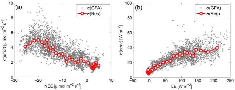
Fig. 1.Data uncertainty derived from the gapfilling algorithm directly and standard deviation of the gapfilling algorithm residuals for NEE

(a)and LE(b).

Fig. 1. Data uncertainty derived from the gapfilling algorithm directly and standard deviation of the gapfilling algorithm residuals for NEE (a) and LE (b).

forest, Hyyti¨al¨a (Finland), an evergreen needleleaf forest and Puechabon (France), an evergreen broadleaf forest. For the parameter retrieval experiments we chose two sites, Hainich and Loobos. The data sets were processed using the stan-dardized methodology described in Papale et al. (2006); Re-ichstein et al. (2005). CO2fluxes are corrected for storage, low turbulence conditions are filtered using theu∗ criteria and spikes (outliers) are detected. Subsequently gap filling and fluxpartitioning is applied. For the parameter estima-tion only filtered and corrected high quality measurements are used.

2.3 Observation errors

In this study we assume that the measurement value consists of the actual value and an additive systematic and random error

x=F +δ+, (1)

whereδ is a systematic error and is a random error. The commonly used ordinary least squares (OLS) optimization assumes the random error standard deviation, e.g. the data uncertainty to be constant (homoscedasticity). A constant standard deviation, can usually be provided by the manufac-turer of a measurement device or it can be determined with simple tests. For flux data the standard deviation of the ran-dom error is not constant in this case tests need to be per-formed for varying conditions, quantifying the changes of the standard deviation. One option is to perform measure-ments close to each other, temporally or spatially, provided that the conditions are the same or very similar, then the ac-tual value is equal and the variation is caused by the random error. For the flux data meteorological conditions, the state of the vegetation and if spatially seperated the footprint and topography have to be comparable. To get an estimate of the random error we used the gapfilling algorithm of Reich-stein et al. (2005). This tool computes the expected value of

the flux using data measured under the same meteorological conditions in a time window of±7 days. The small time win-dow is necessary to ensure a similar condition of the ecosys-tem. The residual of the gap filling algorithm can be used as a random error estimate (Moffat et al., 2007), it is compa-rable to the paired observations approach used in Hollinger and Richardson (2005), as shown in Richardson et al. (2007). For the parameter estimation an error standard deviation has to be assigned to each observation. For the parameter esti-mation experiments we compared the different estimates for the standard deviation of the random error:

1. constant weights,

2. the standard deviations of the observations with simi-lar meteorological conditions within a time window of

±7 days is used directly from the gapfilling algorithm (std),this is equal to the standard deviation of the resid-uals between observations with similar meteorological conditions and expected value,

3. the standard deviations of the residuals of the gapfilling algorithm (res) were obtained grouping the data accord-ing to the flux magnitude in 30 groups with an equal number of data points, for each group the standard de-viation was computed (see Fig. 1). Afterwards the stan-dard deviation was related to the flux magnitude using two linear regression lines to allow for a minimum for net ecosystem exchange of carbon (NEE) and one linear regression line for the latent heat (LE).

1314 G. Lasslop et al.: Influences of observation errors on parameter estimation 2.4 Parameter estimation

The procedure of parameter estimation can be described as varying the parameters until the best fit between model and data is found. The fit or misfit between model and data is quantified via the costfunction:

J (p)=(xd−xm)TCd−1(xd−xm) (2)

xd represents the data vector, xm the model output vector,

Cdthe error covariance matrix andpis the parameter vector.

The best parameter set is found at the minimum of the cost function. T denotes that the vector is transposed. For un-correlated errors the function simplifies, as all off diagonal elements of the matrix Cdare zero, to:

J (p)=

N X

i=1

xdi−xmi

σdi

2

(3) σd is the standard deviation of the random errors, N the

number of data points. In this study we use synthetic data based on a model output, therefore the model error is zero. To consider the uncertainty of flux measurements is neces-sary if the errors are hetereoscedastic, e.g. error variance (=squared standard deviation) increases with increasing flux magnitude, or if different data sources are used. From an-other point of view this means that data with high uncer-tainty (high error variance) get a lower weight than data with low uncertainty (low error variance). For constant error vari-ance the Eq. (3) simplifies to the OLS method summing up only the squared distances. Given a double exponential dis-tribution as proposed by Hollinger and Richardson (2005) and Richardson et al. (2006), parameter estimation should be based on the sum of absolute deviations rather than on squares. To find the minimum of the costfunction we used the Levenberg-Marquardt algorithm implemented in the data analysis package “PV-WAVE 8.5 advantage” (Visual Numer-ics, 2005) for the simple models. For the complex BETHY model a Bayesian approach was used to determine the a pos-teriori probability density function (PDF) of parameters in-cluding prior information and the Metropolis Markov Chain Monte Carlo (MCMC) technique was used to sample the PDF of parameters, which was then characterised by mean and 95% confidence intervalls (Knorr and Kattge, 2005). The Optimisation Intercomparison of Trudinger et al. (2007) compared different algorithms, including the two used here, for the optimisation of a simple coupled model. The opti-misation algorithms were found to be comparable with re-spect to the parameter retrival. We used the MCMC for the complex model with more parameters, since the cost func-tion for the optimizafunc-tion of complex models is more likely to show multiple local minima. For the same reason prior in-formation about the parameters was included for the BETHY model. The LM is suitable for simpler models, as the shape of the cost function does not show many local minima and is then, in spite of the bootstrapping, computationally much more effective.

2.5 Evaluation of the parameter estimation performance The reestimation of the parameters was evaluated through the deviation from the original parameter value, the param-eter uncertainty and the root mean squared error between model output computed with the reestimated parameters and the reference model output without noise. The uncertainty of the parameters determined with the Levenberg-Marquardt algorithm, was derived by bootstrapping (n=500), which is only based on the empirical sample not on assumptions about probability theory of the normal distribution (Wilks, 1995). As a measure of uncertainty for the parameters we used the 95% confidence intervall (=1.96·standard error) of the mean of the parameter distribution. When using the Metropolis algorithm the parameter uncertainties can be directly calcu-lated from the sampling of the MCMC approach. The uncer-tainty reduction when using the Metropolis algorithm was computed as 1−posterior uncertainty

prior uncertainty .

The main difference between bootstrapping and MCMC lies in how they derive the uncertainty. Bootstrapping changes the data, e.g. drawing subsamples from the data, and uses the changes in the parameters to derive the uncertainty while MCMC changes the parameters and uses the model-data mismatch to derive the parameter distribution.

2.6 Models

2.6.1 Hyperbolic light response curve

The Hyperbolic light response curve (HLRC) computes net ecosystem exchange of CO2(NEE) depending on global ra-diation (Rg, incoming shortwave radiation):

NEE= − α·β·Rg

α·Rg+β

+γ (4)

α is an approximation of the canopy light utilization effi-ciency,β is GPP (Gross primary production) at light satu-ration andγ is the ecosystem respiration. Instead ofRg

pho-tosynthetic active radiation (PAR) or phopho-tosynthetic photon flux density (ppfd) is often used, they are closely related to Rg, but not measured at all EC sites. Using Rg instead of

PAR or ppfd changes only the value of α, as PPFD is ap-proximately twice theRg.

2.6.2 Water use efficiency model

To increase the complexity of the model we coupled NEE with the latent energy (LE) using the HLRC and connect-ing it to LE via the water use efficiency (WUE), which is the ratio of gross primary production and latent heat. The WUE times water vapour deficit (WUE VPD) is considered constant (Beer et al., 2007). Using VPD as additional driver NEE and LE can be connected as follows:

NEE= − α·β·Rg

α·Rg+β

LE=(γ −NEE)· VPD

WUE VPD. (6)

This model is inverted against NEE and LE. To make sure, that the LE and NEE misfits contribute to a similar extend to the cost function when using constant weights, as it is the case when using the data derived estimates of the error stan-dard deviation are used, we scaled the residuals with con-stants c for NEE and LE, respectively. These concon-stants are defined such that the sum of the weighted synthetic error is the same when using the constant and using the std weights, for both NEE and LE:

1 c

X

error=Xerror

std (7)

cdenotes the constant weight, the same weight is used for the inversion of the BETHY model. In Eq. (7) “error” is the er-ror estimated from real data, that was added to the synthetic data.

The model underestimates LE, but as we use the model out-put as reference, by design of the study the model errors are not important. Conclusions about the influence of the data error on model parameterisation are not affected. We used this model to show, that the results derived with the simple model hold for models of various complexities and to me-diate between the very simple HLRC and the quite complex SVAT scheme of BETHY.

2.6.3 BETHY

BETHY is a process-based model of the coupled photosyn-thesis and energy balance system to simulate the exchange of CO2, water and energy between soil, plant canopy and at-mosphere (Knorr and Heimann, 2001). It computes absorp-tion of PAR in three layers, while the canopy air space is treated as a single, well mixed air mass with a single temper-ature. Evapotranspiration and sensible heat fluxes are calcu-lated from the Penman-Monteith equation (Monteith, 1965). Carbon uptake is computed with the model by Farquhar et al. (1980) for C3. The stomata and canopy model of Knorr (2000) simulates canopy conductance in response to PAR, VPD and soil water availability. In the version of BETHY applied here, autotrophic respiration is calculated as a tem-perature modulated fraction of photosynthetic capacity while heterotrophic respiration is based on a basal respiration mod-ulated by soil water availability and air temperature. The in-version set up was the same as in Knorr and Kattge (2005), inverting all 21 parameters simultaneously. The prior uncer-tainties of the parameters were set to 20% of the prior pa-rameter value. For the synthetic datasets the prior papa-rameter were the parameters used to generate the data.

3 Results and discussion

3.1 Statistical properties of the error estimates 3.1.1 Heteroscedasticity

The standard deviation of the error has been derived from the residuals of the gapfilling model, e.g. standard deviation of the residuals depending on the flux magnitude (res), and using the standard deviation of the gapfilling algorithm di-rectly (std). Figure 1 shows the relationship between flux magnitude and error standard deviation for NEE and LE. The standard deviation is not homogeneous, e.g. the errors are heteroscedastic and increase with increasing flux magnitude. Thus the residuals have to be weighted with the reciprocal of the standard deviation of the random errors as already sug-gested by previous studies (Richardson et al., 2006). The magnitude of the error variance is similar for the two meth-ods of deriving the error variance described in the previous section, see Fig. 1, for res the observations needed to be grouped to derive the standard deviation. The res standard deviation for NEE ranges from 1 to 5, for LE from 5 to 40. With the std method the ranges are wider because the data were not grouped. For NEE the standard deviation lies be-tween 0.5 and 9.5, for LE bebe-tween 2.8 and 85. For eddy covariance data it is known, that the error variance increases with increasing flux magnitude, Richardson and Hollinger (2005) showed that the error standard deviation of NEE, not the error itself, not only scales with flux magnitude, but that wind speed also has a fundamental effect on the uncertainty. Thus not the whole variability of the standard deviation can be reproduced when only the flux magnitude is used. An-other source for the higher scatter of the std results is the un-certainty in the estimation of the standard deviations derived directly (std).

3.1.2 Distribution

1316 G. Lasslop et al.: Influences of observation errors on parameter estimation

(a)

(b)

(c)

(e)

(g)

(d)

(f)

(h)

G. Lasslop et al.: Influences of observation errors on parameter estimation 1317

(a) (b)

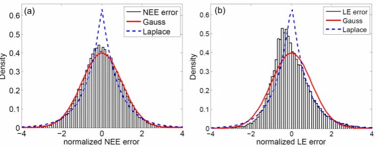
Fig. 3.Distribution of NEE(a)and LE(b)errors normalized with std andztransformed ((error-mean(error))/standarddeviation(error)) using data from HAI, LOO, HYY and PUE.

Fig. 3. Distribution of NEE (a) and LE (b) errors normalized with std andztransformed ((error-mean(error))/standarddeviation(error)) using data from HAI, LOO, HYY and PUE.

16 G. Lasslop et al.: Influences of observation errors on parameter estimation

HAI LOO HYY PUE HAI LOO HYY PUE

(a) NEE (b) LE

Fig. 4. Boxplots with median, upper and lower quartile, minimum and maximum or outliers (points) for the excess kurtosis of the 10 two week periods from May to September 2005 for errors (orig) and normalized errors (norm) of NEE(a)and LE(b).

Fig. 4. Boxplots with median, upper and lower quartile, minimum and maximum or outliers (points) for the excess kurtosis of the 10 two week periods from May to September 2005 for errors (orig) and normalized errors (norm) of NEE (a) and LE (b).

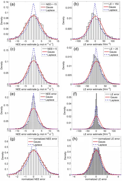
to a standard deviation of unity. For NEE the normalized er-rors are slightly closer to a normal distribution than for LE. Thus the double exponential distribution is largely due to a superposition of Gaussian distributions and the least squares criteria can be used for the eddy covariance data shown here. Figure 3 shows the distribution of errors from the four dif-ferent sites. The normalization of NEE resulted in a rather Gaussian distribution, for LE the distribution is in between Gaussian and Laplace distribution and is slightly skewed. This indicates, that the distribution of the error varies from site to site or that the error estimation does not perform well for all sites. One indicator for the peakedness of the distri-bution is the excess kurtosis (=kurtosis-3), it is zero for a normal distribution and 3 for a double exponential distribu-tion, a high kurtosis indicates a strong peak. Figure 4 shows the kurtosis for ten two week periods for the four sites. For NEE the normalization of the errors decreases the kurtosis and changes the distribution to a less peaked shape. The

1318 G. Lasslop et al.: Influences of observation errors on parameter estimation G. Lasslop et al.: Influences of observation errors on parameter estimation 17

(a) (b)

NEE LE

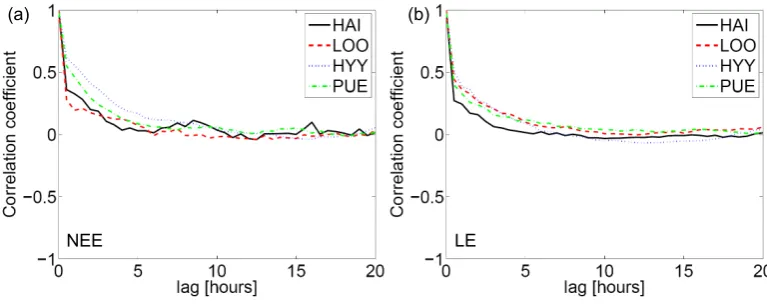
Fig. 5.Autocorrelation of the NEE(a)and LE(b)errors, data: May to September 2005. Fig. 5. Autocorrelation of the NEE (a) and LE (b) errors, data: May to September 2005.

18 G. Lasslop et al.: Influences of observation errors on parameter estimation

(a) NEE (b) LE

Fig. 6.Boxplots of the autocorrelation of lag=1 (0.5 h) for ten two week periods from May to September for NEE(a)and LE(b). Fig. 6. Boxplots of the autocorrelation of lag=1 (0.5 h) for ten two week periods from May to September for NEE (a) and LE (b).

3.1.3 Correlation

Autocorrelation

Figure 5 shows the autocorrelation function of the ran-dom errors for the four eddy sites. The behaviour of the function is similar for all sites, the autocorrelation decays fast, after 10 h there is no considerable change in the correlation. Figure 6 shows boxplots for the autocorrelation for a lag of 30 min, it is usually below 0.7, with one exception for Puechabon (0.82). Hyyti¨al¨a shows the highest autocorrelation for LE and NEE, Loobos the lowest for NEE and Hainich the lowest for LE. Although the gapfilling algorithm provides a reasonable estimate for the random error, the autocorrelation could partly be an artefact of the algorithm, if the deviation from the statistical expectation value was not caused by a random error the following and previous value would deviate in a similar way and the actual autocorrelation of the random error would be

lower. To make sure that error autocorrelation does not influence the parameter estimation one could prefer to use only every second or third value for the parameter estimation. Crosscorrelation

R2 values for the crosscorrelation between NEE and LE errors of the four sites and ten data periods for each site are summarized in Table 1. In our study the corre-lation between NEE and LE errors is close to zero, thus the correlation between NEE and LE errors is of minor importance and does not need to be considered in the error covariance matrix. The highestR2was 0.24 for one period for Puechabon, for the same period the outlier of the LE autocorrelation for a lag of 30 min was found (see Fig. 6).

G. Lasslop et al.: Influences of observation errors on parameter estimation 1319

(a) (b)

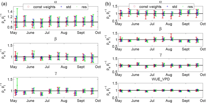
Fig. 7. Time series of normalized parameters (estimated/true) based on data from Loobos with a random error for the HLRC (left) and the WUE model.

Fig. 7. Time series of normalized parameters (estimated/true) based on data from Loobos with a random error for the HLRC (left) and the WUE model.

Table 1. Crosscorrelation between NEE and LE errors for ten two week periods between March and September 2005.

R2of NEE and LE errors

Data 1.– 16.– 1.– 16.– 1.– 16.– 1.– 16.– 1.– 16.– period 15.5. 31.5. 15.6. 30.6. 15.7. 31.7. 15.8. 31.8. 15.9. 30.9. HAI 0.089 0.004 0.176 0.192 0.088 0.136 0.202 0.007 0.077 0.097 LOO 0.004 0.029 0.059 0.086 0.031 0.000 0.004 0.024 0.030 0.010 HYY 0.197 0.033 0.139 0.128 0.021 0.012 0.023 0.049 0.000 0.003 PUE 0.093 0.244 0.038 0.033 0.068 0.003 0.012 0.018 0.019 0.031

errors. This indicates that the variation in the measured fluxes under similar meteorological conditions (i.e. the flux errors) seems to be rather caused by changes in concentrations of water and CO2than by the measurement of the vertical wind velocity. As auto- and crosscorrelation are low, the gener-alized least squares method (Eq. 2) can be simplified to the weighted least squares method (Eq. 3) by setting off-diagonal elements in the error covariance matrix to zero.

3.2 Parameter retrieval

3.2.1 Ordinary least squares vs. weighted least squares The parameters were estimated for three models of differ-ent complexities, the synthetic data is based on data from two different sites (Loobos and Hainich). We are compar-ing constant weights with two ways of estimatcompar-ing the stan-dard deviation of the observation errors, which is then used

1320 G. Lasslop et al.: Influences of observation errors on parameter estimation

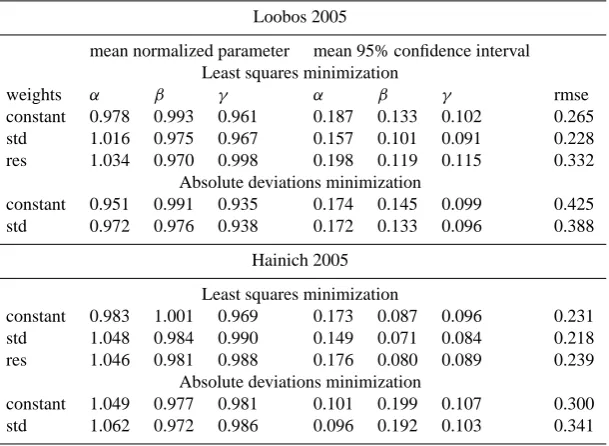
Table 2. Mean of retrieved normalized parameters and the mean uncertainty for the ten two week periods for the HLRC.

Loobos 2005

mean normalized parameter mean 95% confidence interval Least squares minimization

weights α β γ α β γ rmse

constant 0.978 0.993 0.961 0.187 0.133 0.102 0.265 std 1.016 0.975 0.967 0.157 0.101 0.091 0.228 res 1.034 0.970 0.998 0.198 0.119 0.115 0.332

Absolute deviations minimization

constant 0.951 0.991 0.935 0.174 0.145 0.099 0.425 std 0.972 0.976 0.938 0.172 0.133 0.096 0.388

Hainich 2005

Least squares minimization

constant 0.983 1.001 0.969 0.173 0.087 0.096 0.231 std 1.048 0.984 0.990 0.149 0.071 0.084 0.218 res 1.046 0.981 0.988 0.176 0.080 0.089 0.239

Absolute deviations minimization

constant 1.049 0.977 0.981 0.101 0.199 0.107 0.300 std 1.062 0.972 0.986 0.096 0.192 0.103 0.341

Table 3. Mean of retrieved normalized parameters and the mean uncertainty for the ten two week periods for the WUE-model using last squares minimization.

Loobos 2005

mean normalized parameter mean 95% confidence interval

weights α β γ wue vpd α β γ wue vpd rmse const 0.974 1.003 0.964 0.980 0.249 0.149 0.111 0.058 1.243 std 1.043 0.963 0.973 0.987 0.140 0.088 0.085 0.050 0.930 res 1.032 0.958 0.975 0.973 0.148 0.096 0.090 0.054 1.238

Hainich 2005

mean normalized parameter mean 95% confidence interval

weights α β γ wue vpd α β γ wue vpd rmse const 1.027 0.987 0.986 0.960 0.300 0.135 0.166 0.051 2.926 std 1.049 0.978 0.984 0.978 0.121 0.081 0.092 0.043 1.924 res 1.061 0.964 0.986 0.952 0.143 0.090 0.098 0.045 3.330

in which the results are opposite. The std weights decrease the mean uncertainty more than res and therefore describe the error standard deviation better. The root mean squared error (rmse) between reference model output without noise and the model output using the reestimated parameters can be decreased using std as weights for the HLRC, for res it increases. This indicates, that the “std” is a more accurate estimate for the data uncertainty and that a description of the data uncertainty only based on flux magnitude, as “res”, is likely not sufficient. For the water use efficiency model the results of the model parameterization are similar, estimates of parameter uncertainty decrease between 5% and 60% and the RMSE between reference model output and model output of the reestimated parameters is decreased when using std,

G. Lasslop et al.: Influences of observation errors on parameter estimation 1321

(a)

(b)

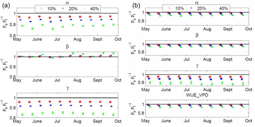
Fig. 8.Time series of normalized parameters (estimated/true) based on data from Loobos with a selective systematic nighttime error for the HLRC(a)and the WUE model(b).

Fig. 8. Time series of normalized parameters (estimated/true) based on data from Loobos with a selective systematic nighttime error for the HLRC (a) and the WUE model (b).

parameters estimated with std weights resulted in reasonable parameters, whereas using constant weights for some peri-ods negative values forαwere estimated for the HLRC and water use efficiency model (not shown). The random error changes the shape of the cost function, it can increase the number of local minima or the minimization can become an ill-posed problem. Using weights representing the data un-certainty seems to improve the behaviour of the cost function and improves the extraction of information inherent to the data. This shows that the standard deviation provided by the gapfilling algorithm is a good measure for the eddy covari-ance data uncertainty, it improves the parameter retrieval and therefore model performance after optimization, at least for the sites used here. For skewed error distributions we would expect the parameter estimates to be biased.

To explore the power of the Bayesian approach an inter-esting alternative way to cope with data uncertainties would be to include a relationship for the data uncertainty in the Likelihood function. The uncertainty could be represented by a linear dependency and the parameters of the relation-ship could be estimated in addition to the model parameters. However, since with eddy covariance data one can provide information about the random error in the data independent of the optimization, we expect our method to be more robust, e.g. independent of model errors.

3.2.2 Least squares vs. absolute deviations

As the use of absolute deviations in the cost function was suggested previously by Richardson et al. (2006) we com-pare least squares and absolute deviations, to illustrate the

Table 4. Sum of the uncertainty reduction, summed absolute devi-ation of the parameter ratio from 1 and mean rmse between model output and reference output for the BETHY model.

site Loobos Hainich

const std const std uncertainty reduction 50.93 52.31 47.19 50.08 parameter deviation 14.83 13.30 14.16 12.49 rmse 4.11 3.17 4.34 3.6

1322 G. Lasslop et al.: Influences of observation errors on parameter estimation 3.2.3 Systematic error

Figure 8 shows the results of the parameter retrieval based on data with a selective systematic nighttime error of 10, 20 and 40%. The α and γ parameters of the HLRC show a systematic bias, estimated parameters underestimate the un-derlying true parameter. The bias is stronger for higher data error. Forβ the parameter bias seems to be not systematic, the retrieved parameter is for some periods lower, for some periods higher than the original parameter.β is GPP at light saturation, as NEE at light saturation does not change but only the night time data point, representing the respiration, is lowerβ should also be lower to sum up to the same NEE values during daytime. The effect onγ seems to be too low to show up in the comparably high values ofβ. For the water use efficiency model all parameters are biased, all estimates are lower than the true values. Through the interconnection of GPP and LE and the use of water and CO2fluxes to con-strain the parameters the distance to the true value decreases for all parameters. This illustrates the potential of using mul-tiple constraints for inverse model parameter estimation. The parameter uncertainties increase the higher the error but the real value of the parameter is not within the uncertainty range of the estimated parameter. This means, that the real uncer-tainty of the parameter is underestimated, projection of the parameter uncertainty to model output will result in tainties for the fluxes that are too low. To get the real uncer-tainty for parameters and fluxes further knowledge about the systematic errors is needed and methods need to be devel-oped to incorporate them into the estimation of uncertainty, if the systematic errors cannot be removed.

4 Conclusions

Previous work to quantify the random error structure of eddy covariance data (Hollinger et al., 2004; Richardson and Hollinger, 2005; Richardson et al., 2006) has focused on de-scribing the moments of the distribution of the error, partic-ularly relating the expected magnitude of the error (i.e. its standard deviation) to the flux magnitude, and evaluating whether or not flux errors are Gaussian. Here we have built on these efforts by considering the auto- and crosscorrelation, introducing a new method to quantify the standard deviation of the random errors. We show the effect of the varying stan-dard deviation to the distribution and investigate how random and systematic errors affect parameter estimates.

The analysis of the error distribution shows that the appar-ently double exponential distribution of the eddy flux data can be almost entirely due to the superposition of Gaussian distributions with inhomogeneous variance. Whether this is the case for a special site can be affirmed by testing the nor-mality of the normalized error distribution. If it cannot be affirmed one should consider using robust methods. The au-tocorrelation is low, but one might consider to analyse the autocorrelation function and use only every second or third

data point for parameter estimation if there is enough data available. As a reason for the low but significant autocorre-lation of errors we can not exclude artefacts of the gap filling tool. The crosscorrelation between LE and NEE is low and can be neglected. The assumption for ordinary least squares that is not met is the constant error standard deviation, thus the ordinary least squares method needs to be extended to weighted least squares, using the reciprocal of the standard deviation as weight in the costfunction. We propose a mea-sure for data uncertainty, e.g. the standard deviation of the values used to compute the expected value, that can be used to weight the data in the costfunction. Weighting the data decreases the parameter uncertainty and the parameter re-trieval is improved. We showed that this result holds true for a wide range of model complexities. We show that the impact of systematic errors varies by parameter, but the bias is systematic, therefore the interpretation of parameters de-rived from data with systematic errors might be misleading. The parameter uncertainty slightly increases when a system-atic error is added, but the true parameter is not within the uncertainty range of the estimate. Not considered here but of similar importance is the model error, which was set to zero by using the model output as basis for the synthetic data. For the least squares optimization the model output random er-ror is additive to the data random erer-ror and depending on the point of view part of the data random error can also be seen as model errors, e.g. footprint heterogeneity. Model struc-tural problems can also affect parameter estimation in a sim-ilar way as systematic data errors, i.e. dynamics in the data that are not represented or not sufficiently represented in the model structure can lead to parameters with biases, which are not reflected in their uncertainty estimates (Carvalhais et al., 2008). Hence we conclude that potential systematic errors in flux data or models need to be addressed more thoroughly in data assimilation approaches since otherwise uncertainties will be vastly underestimated.

Acknowledgements. We would like to thank T. Vesala, W. Kutsch, E. J. Moors and S. Rambal, whose data have contributed to this study. This work would have been impossible without the integrated project “Carboeurope” (GOCECT2003-505572) of the European Union (EU). This research was funded in part by the Marie Curie European Reintegration Grant “GLUES” (MC MERG-CT-2005-031077). GL and MR would like to thank the Max-Planck Society for supporting the “Biogeochemical Model-Data Integration Group” as an Independent Junior Research Group. DP thanks also the “Cooperazione Italia-USA su Scienza e Tecnologia dei cambiamenti climatici – Anno 2006-2008” CMCC project for the support. We are grateful to A. Richardson, N. Carvalhais and T. Foken for valuable comments, discussions and the careful reading of the manuscript and E. Tomelleri for discussions about Metropolis. We also would like to thank the anonymous reviewer and Luigi Renzullo for their comments and criticism, which have greatly helped to improve the paper.

References

Baldocchi, D. D., Falge, E., Gu, L., Olson, R., Hollinger, D. Y., Running, S. W., Anthoni, P., Bernhofer, C., Davis, K. J., Evans, R., Fuentes, J., Goldstein, A., Katul, G., Law, B. E., Lee, X., Malhi, Y., Meyers, T. P., Munger, J. W., Oechel, W. C., Paw U, K. T., Pilegaard, K., Schmid, H. P., Valentini, R., Verma, S., Vesala, T., Wilson, K. B., and Wofsy, S. C.: FLUXNET: A New Tool to Study the Temporal and Spatial Variability of Ecosystem-Scale Carbon Dioxide, Water Vapor, and Energy Flux Densities, B. Am. Meteorol. Soc., 82, 2415–2434, 2001.

Beer, C., Reichstein, M., Ciais, P., Farquhar, G. D., and Papale, D.: Mean annual GPP of Europe derived from its water balance, Geophys. Res. Lett., 34, L05401, doi:10.1029/2006GL029006, 2007.

Braswell, B., Sacks, W., Linder, E., and Schimel, D.: Estimating diurnal to annual ecosystem parameters by synthesis of a carbon flux model with eddy covariance net ecosystem exchange obser-vations., Glob. Change Biol., 11, 335–355, 2005.

Carvalhais, N., Reichstein, M., Seixas, J., Collatz, G.J., Santos Pereira, J., Berbigier, P. Carrara, A., Granier, A., Montagnani, L., Papale, D., Rambal, S., Sanz, M. J., Valentini, R.: Implications of Carbon Cycle Steady State Assumptions for Biogeochemical Modeling Performance and Inverse Parameter Retrieval, Global Biogeochem. Cy., 22, doi:10.1029/2007GB003033, 2008. Draper, N. and Smith, H.: Applied Regression Analysis, Wiley,

New York, third edition, 736 pp., 1998.

Evans, G. T.: Defining misfit between biogeochemical models and data sets, J. Marine Syst., 40–41, 49–54, 2003.

Farquhar, G. D., von Caemmerer, S., and Berry, J. A.: A biochemi-cal model of photosynthesis in leaves of C3 species, Planta, 149, 78-90, 1980.

Friend, A. D., Arneth, A., Kiang, N. Y., Lomas, M., Ogee, J., Ro-denbeck, C., Running, S. W., Santaren, J.-D., Sitch, S., Viovy, N., Woodwards, F. I., and Zaehle, S.: FLUXNET and modelling the global carbon cycle, Glob. Change Biol., 13, 610–633, 2007. Hollinger, D. and Richardson, A.: Uncertainty in eddy covariance measurements and its application to physiological models, Tree Physiol., 25, 873–885, 2005.

Hollinger, D. Y., Aber, J., Dail, B., Davidson, E. A., Goltz, S. M., Hughes, H., Leclerc, M. Y., Lee, J. T., Richardson, A. D., Ro-drigues, C., Scott, N., Achuatavarier, D., and Walsh, J.: Spa-tial and temporal variability in forest-atmosphere CO₂exchange, Glob. Change Biol., 10, 1689–1706, 2004.

Knorr, W.: Annual and interannual CO₂exchanges of the terrestrial biosphere: process-based simulations and uncertainties, Global Ecol. Biogeogr., 9, 225–252, 2000.

Knorr, W. and Heimann, M.: Uncertainties in global terrestrial biosphere modelingUncertainties in global terrestrial biosphere modeling. Part I: a comprehensive sensitivity analysis with a new photosynthesis and energy balance scheme, Global Biogeochem. Cy., 15, 207–225, 2001.

Knorr, W. and Kattge, J.: Inversion of terrestrial ecosystem model parameter values against eddy covariance measurements by Monte Carlo sampling, Glob. Change Biol., 11, 1333–1351, 2005.

Moffat, A. M., Papale, D., Reichstein, M., Hollinger, D. Y., Richardson, A. D., Barr, A. G., Beckstein, C., Braswell, B. H., Churkina, G., Desai, A. R., Falge, E., Gove, J. H., Heimann, M., Hui, D., Jarvis, A. J., Kattge, J., Noormets, A., and Stauch,

V. J.: Comprehensive comparison of gap-filling techniques for eddy covariance net carbon fluxes, Agr. Forest Meteorol., 147, 209–232, 2007.

Moncrieff, J., Malhi, Y., and Leuning, R.: The propagation of errors in long-term measurements of land-atmosphere fluxes of carbon and water, Glob. Change Biol., 2, 231–240, 1996.

Monteith, J. L.: Evaporation and environment, Symposium of the Society for Experimental Biology, 19, 205-234, 1965.

Owen, K. E., Tenhunen, J., Reichstein, M., Wang, Q., Falge, E., Geyer, R., Xiao, X., Stoy, P., Ammann, C., Arain, A., Aubinet, M., Aurela, M., Bernhofer, C., Chojnicki, B. H., Granier, A., Gruenwald, T., Hadley, J., Heinesch, B., Hollinger, D., Knohl, A., Kutsch, W., Lohila, A., Meyers, T., Moors, E., Moureaux, C., Pilegaard, K., Saigusa, N., Verma, S., Vesala, T., and Vo-gel, C.: Linking flux network measurements to continental scale simulations: ecosystem carbon dioxide exchange capacity under non-water-stressed conditions, Glob. Change Biol., 13, 734–760, 2007.

Papale, D., Reichstein, M., Aubinet, M., Canfora, E., Bernhofer, C., Kutsch, W., Longdoz, B., Rambal, S., Valentini, R., Vesala, T., and Yakir, D.: Towards a standardized processing of Net Ecosys-tem Exchange measured with eddy covariance technique: algo-rithms and uncertainty estimation, Biogeosciences, 3, 571–583, 2006, http://www.biogeosciences.net/3/571/2006/.

Raupach, M. R., Rayner, P. J., Barrett, D. J., DeFries, R. S., Heimann, M., Ojima, D. S., Quegan, S., and Schmullius, C. C.: Model-data synthesis in terrestrial carbon observation: meth-ods, data requirements and data uncertainty specifications, Glob. Change Biol., 11, 378–397, 2005.

Reichstein, M., Tenhunen, J., Roupsard, O., Ourcival, J. M., Rambal, S., Miglietta, F., Peressotti, A., Pecchiari, M., Tirone, G., and Valentini, R.: Inverse modeling of seasonal drought effects on canopy CO2/H2O exchange in three Mediter-ranean ecosystems, J. Geophys. Res.-Atmos., 108, D23, 4726, doi:10.1029/2003JD003430, 2003.

Reichstein, M., Falge, E., Baldocchi, D., Papale, D., Aubinet, M., Berbigier, P., Bernhofer, C., Buchmann, N., Gilmanov, T., Granier, A., Grunwald, T., Havrankova, K., Ilvesniemi, H., Janous, D., Knohl, A., Laurila, T., Lohila, A., Loustau, D., Mat-teucci, G., Meyers, T., Miglietta, F., Ourcival, J. M., Pumpanen, J., Rambal, S., Rotenberg, E., Sanz, M., Tenhunen, J., Seufert, G., Vaccari, F., Vesala, T., Yakir, D., and Valentini, R.: On the separation of net ecosystem exchange into assimilation and ecosystem respiration: review and improved algorithm, Glob. Change Biol., 11, 1424–1439, 2005.

Richardson, A. D. and Hollinger, D. Y.: Statistical modeling of ecosystem respiration using eddy covariance data: Maximum likelihood parameter estimation, and Monte Carlo simulation of model and parameter uncertainty, applied to three simple models, Agr. Forest Meteorol., 131, 191–208, 2005.

Richardson, A. D., Hollinger, D. Y., Burba, G. G., Davis, K. J., Flanagan, L. B., Katul, G. G., Munger, J. W., Ricciuto, D. M., Stoy, P. C., Suyker, A. E., Verma, S. B., and Wofsy, S. C.: A multi-site analysis of random error in tower-based measurements of carbon and energy fluxes, Agr. Forest Meteorol., 136, 1–18, 2006.

Statisti-1324 G. Lasslop et al.: Influences of observation errors on parameter estimation

cal properties of random CO₂flux measurement uncertainty in-ferred from model residuals, Agr. Forest Meteorol., 148, 38–50, doi:10.1016/j.agrformet.2007.09001, 2007.

Sacks, W. J., Schimel, D. S., Monson, R. K., and Braswell, B. H.: Model-data synthesis of diurnal and seasonal CO2fluxes at Ni-wot Ridge, Colorado, Glob. Change Biol., 12, 240–259, 2006. Tarantola, A.: Inverse Problem Theory: Methods for Data Fitting

and Model Parameter Estimation, Elsevier, New York, 1st ed., 613 pp., 1987.

Trudinger, C. M., Raupach, M. R., Rayner, P. J., Kattge, J., Li, Q., Pak, B., Reichstein, M., Renzullo, L., Richardson, A. D., Roxburgh, S. H., Styles, J., Wang, Y. P., Briggs, P., Barrett, D., and Nikolova, S.: OptIC project: An intercomparison of optimization techniques for parameter estimation in terrestrial biogeochemical models, J. Geophys. Res., 112, G2, G02027, doi:10.1029/2006/JG000367, 2007.

Visual Numerics, Inc.: PV-Wave 8.5 Reference Guide, Houston, http://www.vni.com/books/dod/pdf/wave85Docs/ eReferenceGuide85.pdf, last access: 9 September 2008, 2005. Wang, Y. P., Baldocchi, D., Leuning, R., Falge, E., and Vesala, T.:

Estimating parameters in a land-surface model by applying non-linear inversion to eddy covariance flux measurements from eight FLUXNET sites, Glob. Change Biol., 13, 652–670, 2007. Wilks, D. S.: Statistical Methods in the Atmospheric Sciences,

Aca-demic Press, 467 pp., 1995.