Annales
Geophysicae
Ionospheric energy input as a function of solar wind parameters:
global MHD simulation results
M. Palmroth1, P. Janhunen1, T. I. Pulkkinen1, and H. E. J. Koskinen2,1 1Finnish Meteorological Institute, Geophysical Research Division, Finland 2University of Helsinki, Department of Physical Sciences, Finland
Received: 17 December 2002 – Revised: 29 April 2003 – Accepted: 18 June 2003 – Published: 1 January 2004
Abstract. We examine the global energetics of the solar wind magnetosphere-ionosphere system by using the global MHD simulation code GUMICS-4. We show simulation re-sults for a major magnetospheric storm (6 April 2000) and a moderate substorm (15 August 2001). The ionospheric dis-sipation is investigated by determining the Joule heating and precipitation powers in the simulation during the two events. The ionospheric dissipation is concentrated largely on the dayside cusp region during the main phase of the storm pe-riod, whereas the nightside oval dominates the ionospheric dissipation during the substorm event. The temporal vari-ations of the precipitation power during the two events are shown to correlate well with the commonly usedAE-based proxy of the precipitation power. The temporal variation of the Joule heating power during the substorm event is well-correlated with a commonly usedAE-based empirical proxy, whereas during the storm period the simulated Joule heating is different from the empirical proxy. Finally, we derive a power law formula, which gives the total ionospheric dis-sipation from the solar wind density, velocity and magnetic fieldz-component and which agrees with the simulation re-sult with more than 80% correlation.
Key words. Ionosphere (modeling and forecasting) – Magnetospheric physics (magnetosphere-ionosphere interac-tions; storms and substorms)
1 Introduction
The energy transfer process between the solar wind and the magnetosphere and further between the ionosphere is one of the key questions in space physics, frequently brought up in executive summaries of many proposals and space physics research strategy reports (e.g. Acu˜na et al., 1995). While the energy transfer process was qualitatively explained al-ready in the 1960’s by the first theories of the solar wind-magnetosphere coupling (Dungey, 1961; Axford and Hines,
Correspondence to: M. Palmroth ([email protected]
1961), the quantitative assessment of the problem has proven to be difficult. The energy transfer mechanism by which the solar wind energy enters the magnetosphere has been ex-plained by magnetic reconnection and viscous interaction. The amount of transferred energy is still uncertain, because the results rely on correlations of solar wind parameters with known dissipation channels inside the magnetosphere (e.g. Akasofu, 1981). The first quantitative attempt using a global MHD simulation to identify both the amount of energy ferred through the magnetopause as well as the energy trans-fer locations at the magnetopause was made by Palmroth et al. (2003). They found that during southward interplan-etary magnetic field (IMF) the locations of energy transfer are controlled by the focusing of the Poynting vector in the plane of the IMF clock angle (see also Papadopoulos et al., 1999). On the other hand, during northward IMF the Poynt-ing flux focusPoynt-ing does not play a major role in determinPoynt-ing the energy transfer locations, as reconnection may not have opened the magnetopause at the locations where the Poynt-ing vector focuses (Palmroth et al., 2003).
The dissipation of the solar wind energy, both during mag-netospheric substorms and magnetic storms, in the various sinks in the magnetosphere and the ionosphere, has also been a subject of several past studies (Akasofu, 1981; Weiss et al., 1992; Lu et al., 1998; Turner et al., 2001; Pulkkinen et al., 2002). The understanding of the relative importance of the various sinks has changed over the years. For a long time the ring current was assumed to be the largest sink (Aka-sofu, 1981), whereas the more recent studies suggest that the polar ionosphere plays a major role in dissipating the solar wind energy (e.g. Weiss et al, 1992 and references therein). In the ionosphere the two largest dissipation mechanisms are the Ohmic Joule heating in the ionosphere, when the field-aligned currents are closed across the equipotential surfaces, and the energy deposition by particles precipitating in the au-roral region of the ionosphere.
the particle precipitation have substantially increased from the 1% assumed originally (e.g. Akasofu, 1981). At present, there are no direct ways to measure the energy deposited by Joule heating, only statistical estimates exist (e.g. Ahn et al., 1983), which give the amount of energy based on the ground magnetic variations caused by the auroral electrojets (such as theAEindex). TheAEindex-based methods are only as good as the ability of theAEindex to describe the tempo-ral and spatial variations of the Pedersen currents not only within the auroral regions, but in the polar cap as well. As theAEstations are located at high latitudes, the true inten-sity of the auroral electrojets is not recorded, particularly dur-ing major storms when the auroral oval moves significantly equatorward.
Measuring the energy deposited by particle precipitation is easier than measuring the energy deposited by Joule heating. When precipitating into the ionosphere, particles collide with atmospheric particles which emit auroral light that can be di-rectly measured on the ground or from polar-orbiting satel-lites. A method based on ultraviolet image measurements on board the Polar satellite was described by Østgaard et al. (2002). To generalize their results, they fitted the precipi-tation energy to the ALindex. While this gives an easily available proxy for the precipitation power, it leads to sim-ilar problems related to theAE-based proxies as described above. On the other hand, the statistical distribution of elec-tron precipitation can also be measured directly by polar-orbiting satellites. For example, Newell et al. (1996) found that the probability of observing accelerated electron precip-itation is increased mainly in 18:00–24:00 MLT sector in the nightside. The latitudinal extent of the precipitation depends strongly on the level of magnetic variation. During large storms the oval moves equatorward, while during quiet times the auroral luminosity is concentrated on high latitudes.
There are only a few studies reporting on the energy depo-sition rate into the ionosphere using global models. Lu et al. (1998) were the first to apply the assimilative mapping of ionospheric electrodynamics (AMIE) technique to estimate the energy deposition rate into the ionosphere during a mag-netic storm. The AMIE procedure is based on the mapping procedure by Richmond and Kamide (1988), and it utilizes several models and a variety of measurements in an assim-ilative way. From the AMIE output Lu et al. (1998) derived the Joule heating and precipitation powers in the ionosphere and concluded that the temporal variation of the Joule heat-ing and precipitation power resembled that of theAEindex. Lu et al. (1998) determined the globally integrated average of Joule heating rate as 190 GW and the average precipita-tion power as about 90 GW during the particular storm they analyzed.
The global MHD simulations can also be used to in-vestigate the energy flow in the coupled solar wind-magnetosphere-ionosphere system. The recent development of the global MHD simulations has focused on the predic-tion of the magnetospheric state from a given solar wind in-put, while systematic examination of the magnetospheric re-sponse to given solar wind still awaits to be done. Several
attempts along this direction have shown to be useful, par-ticularly in cases where the parameters describing the solar wind-magnetosphere-ionosphere coupling are either difficult or impossible to measure globally. For example, the global MHD simulations have been used in mapping the Poynting flux from the solar wind into the magnetosphere to examine the energy flow paths (e.g. Walker et al., 1993; Papadopoulos et al., 1999).
This paper is a continuation of the work by Palmroth et al. (2003), who developed a quantitative method to deter-mine the energy transfer across the magnetopause in a global MHD simulation. Here we calculate the ionospheric energy dissipation, namely the Joule heating and precipitation pow-ers, in the GUMICS-4 global MHD simulation. We deter-mine the latitudinal and longitudinal distributions of the dis-sipated energy, as well as the temporal variation of the global ionospheric dissipation. We analyze results from two sim-ulated events, a magnetic storm that occurred on 6–7 April 2000, and a substorm that occurred on 15 August 2001. Our final aim is to develop a simple relationship between the solar wind input and ionospheric output. In Sect. 2 we introduce the GUMICS-4 global MHD simulation and the calculation of the ionospheric Joule heating and the precipitation powers; furthermore, we examine theoretically how the ionospheric output depends on solar wind parameters in an ideal MHD. Section 3 describes the observations and the simulation re-sults for the two events. In Sect. 4 we present the rere-sults, i.e. the calculated energy dissipation and the latitudinal and longitudinal dissipation distributions for the two events. In Sect. 4.4 we present the fit of the solar wind input data to calculated ionospheric output. Finally, in Sect. 5 we summa-rize our results and end with a discussion.
2 Model description
2.1 GUMICS-4 global MHD simulation
GUMICS-4 (Janhunen, 1996) is a global 3-dimensional MHD simulation code that couples the solar wind-magnetosphere-ionosphere system in a simulation box with an automatically adaptive Cartesian octogrid.Automatical adaption means that whenever the code detects large gradi-ents the cells near the gradigradi-ents are divided into 8 daugh-ter cells. The adaptation depends further on location, such that near-Earth cells are more easily refined than, for ex-ample, cells at the distant tail. The GUMICS-4 simula-tion solves the fully conservative MHD equasimula-tions in the so-lar wind-magnetosphere domain, whereas electrostatic equa-tions are solved in the ionospheric domain. The simula-tion box reaches fromXGSE = 32RE upwind toXGSE = −224RE in the antisunward direction, and in theYGSE and ZGSE directions to ±64RE. The lower limit of the
mag-netospheric domain is a 3.7RE-radius spherical shell from
The ionospheric electron density is affected by the solar extreme ultraviolet radiation, as well as the electron precipi-tation from the magnetosphere, which is assumed to orginate from a Maxwellian source population. The Pedersen and Hall conductivities are computed from the electron density in a three-dimensional grid using 20 non-uniform height lev-els. The electrostatic potential equation is solved in the ionosphere using the height-integrated conductivities and the field-aligned current from the magnetosphere, after which the ionospheric potential is mapped back to the inner bound-ary of the magnetosphere and used as a boundbound-ary condition for the MHD equations. The spherical ionosphere uses a tri-angular fixed grid, in which the oval region is more refined (grid resolution of about 100 km×100 km) than, for exam-ple, in the equatorial region.
The simulations of the two events were carried out in a code setup similar to that described in Palmroth et al. (2001). In the April 2000 storm simulation the IMF Bx was set to
zero to ensure the divergence-free input magnetic field. In the 15 August 2001 substorm simulation the IMF Bx was
set to a constant value of−3 nT, which corresponds to the observed value of IMF Bx before 5:00 UT. Consequently,
the input magnetic field at the time of onset (∼04:30 UT) was modeled accurately. Of course, constantBxalso fulfills
the divergence-free condition. In the April 2000 storm sim-ulation the smallest grid size was 0.5RE, whereas in the 15
August 2001 substorm simulation the smallest grid size was 0.25RE. The denser grid resolution in the magnetosphere
typically tends to increase the polar cap potentials, which are typically 20−30% smaller in GUMICS-4 (with 0.5RE as
the smallest grid) than in, for example, SuperDARN obser-vations.
2.2 Energy dissipated into the ionosphere
The ionospheric dissipation is calculated as a sum of the power consumed by Joule heatingPJ H and the precipitating
particles. The Joule heating power is calculated as PJ H =
Z
E·JdS=
Z
6PE2dS, (1)
where E is the electric field, J the height-integrated cur-rent density,6P the height-integrated Pedersen conductivity,
anddSthe area element on the spherical ionospheric surface. The quantities are interpolated from the simulation results in an ionospheric grid with a resolution of 1◦in latitude and 3◦ in longitude. This interpolation is a necessary operation due to the non-uniform grid utilized by the simulation code, and it does not affect the integration results.
The energy associated with particle precipitation is ob-tained using formulas given by Robinson et al. (1987), where the height-integrated ionospheric Pedersen and Hall conduc-tivities,6P and6H, are calculated using the energy flux and
the average energy of precipitating electrons. In the present study, we obtain the height-integrated conductivities from the simulation results and analytically invert Eqs. (3) and (4) of Robinson et al. (1987) to obtain the precipitation energy flux.
2.3 Similarity scaling laws
Consider the ideal MHD equations written in the primitive variable form
∂tρ= −∇ ·(ρv) (2)
ρ (∂tρ+v· ∇v)= −∇P +j×B (3)
∂tB= ∇ ×(v×B) (4)
(∂t +v· ∇) (Pρ−γ)0, (5)
wherej = ∇ ×B/µ0. Furthermore, let us concentrate on stationary solutions (∂t =0), and decomposeB=B0+B1, where B0 is the Earth’s internal field and B1 is the exter-nally induced part. Then, any solution of Eqs. (2-5) is de-fined by four functions of three coordinatesρ(x),v(x), P (x)
and B1(x). The similarity scalings of such solutions are
new solutionsρ0(x),v0(x), P0(x)andB0
1(x)which are re-lated to the original ones byρ0(CLx)=Cρρ(x),v0(CLx)=
Cvv(x),P0(CLx)= CPP (x)andB01(CLx) =CB1B1(x),
whereCρ,Cv,CP andCB1 are the scaling factors for
den-sity, velocity, pressure and perturbation magnetic field, and CLis the scaling factor for spatial coordinates. We also
in-troduce a scaling factorCB0 for the internal magnetic field in
the same way as for the dynamic variables, and require that the new functions satisfy Eqs. (2–5) with∂t =0. In the
sta-tionary case, Eqs. (2) and (5) contain only one term and thus do not imply any conditions for the scaling factors, but the momentum equation (3) and Faraday’s law (4) read
ρv·∇v− 1
µ0(∇ ×B1)×B0− 1
µ0(∇ ×B1)×B1+∇P =0(6) ∇ ×(v×B0)+ ∇ ×(v×B1)=0. (7) Applying the scalings and requiring that each possible pair of the terms in Eqs. (6) and (7) scales in the same way we obtain the conditions
CρCv2=CB1CB0 =C
2
B1 =CP, (8)
i.e. CB0 = CB1 = C
1/2
ρ Cv, CP = CρC2v. Requiring that
the internal field is the dipole field which scales asr−3we obtain the connectionCL =CB−1/3
0 between the coordinate
scalingCLand the internal field scalingCB0. We thus see
thatCρ andCv can be selected freely but the other scaling
factors CB1, CB0, CP andCL follow from these two. In
other words, by starting from a stationary solution which is valid for solar wind densityρ and velocityv, we obtain a two-parameter family of similarity solutions which spans all possible solar wind density and velocity combinations. The nature of the similarity solutions is such that if, for exam-ple, the solar wind density is multiplied by 10, the density and pressure everywhere in the simulation box are also mul-tiplied by 10, the magnetic fields by
√
-20 -100
10 20 30
IMF Bz [nT]
0 60 120 180 240 300 360
IMF cloc
k
angle [deg]
0 10 20 30
SW pd
yn [nP
a]
0 500 1000 1500 2000 2500
AE(86) [nT]
-300 -200 -100 0
Final Dst [nT]
Time of April 6, 2000 [hrs] (a)
(b)
(c)
(d)
(e)
0 5 10
Epsilon [
10
12 W]
0 20 40
14 16 18 20 22 24 02 04 06 08
Es
[10
12 W]
[image:4.595.50.283.63.517.2](g) (f)
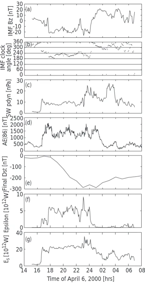
Fig. 1. Solar wind conditions during the April 2000 storm. (a) IMF
Bz, (b) IMF clock angle, (c) solar wind dynamic pressure, (d)AE
index measured at 86 stations, (e) finalDst index, (f)calculated from the solar wind parameters, and (g) total energy through the magnetopause surface.
Apart from the changing ionospheric feedback and the in-herent time-dependence of the solution, the similarity solu-tions should, therefore, correspond to what we obtain from GUMICS-4.
The ionospheric Joule heating is proportional to the square of the current flowing through the ionosphere, if the iono-spheric conductivity pattern and the geometry of the current stay constant. The Joule heatingPJH is given by an iono-spheric area integralPJH =
R
dSJP2/6P, where 6P is the
height-integrated Pedersen conductivity andJPis the
height-integrated Pedersen current. The MHD similarity solutions
scale such that the polar cap expands or shrinks but the rent pattern stays approximately self-similar. If the total cur-rentI flowing through the ionosphere is kept constant,JP
is proportional toI /RP C, where RP C is the polar cap
ra-dius. Since the polar cap area is proportional toRP C2 , the Joule heating PJH is independent ofRP C. Thus, we
con-clude that, approximately,PJHis proportional toI2. The total currentI flowing through the ionosphere scales in the same way as the magnetospheric current systems, thus we obtain I ∼j L2, where the current densityj ∼B1/LandLis the spatial length, i.e.I ∼(B1/L)L2 =B1L ∼P1/2P−1/6 = P1/3, where P is the solar wind dynamic pressure. Thus, PJH∼P2/3∼(ρv2)2/3∼ρ2/3v4/3.
The ionospheric particle precipitation energy flux per unit area from a magnetospheric Maxwellian source plasma is proportional toPt hvt h, wherePt his the thermal pressure of
the source plasma andvt h∼vits thermal velocity (Janhunen
and Olsson, 1998). Thus, the total power of particle precipi-tationPprecscales asPprec ∼Pt hvt hAPC ∼ρv3APC, where APCis the polar cap area. In a dipole field a simple consid-eration shows thatAPC∼L−1∼P1/6∼(ρv2)1/6and thus Pprec∼ρ7/6v10/3.
To summarize, we have obtained that PJH∼ρ2/3v4/3
Pprec∼ρ7/6v10/3
I ∼P1/3, (9)
whereρandvare the solar wind density and velocity, respec-tively,P =ρv2is the dynamic pressure, andPJHandPprec are the total Joule heating and particle precipitation powers, respectively.
3 Event descriptions
3.1 6–7 April 2000 storm
Figure 1 presents the 6–7 April 2000 storm observations, as well as the energy input to the magnetosphere using GUMICS-4 simulation and an empirical parameter. Fig-ures 1a–e show, respectively, the IMF Bz component, the
IMF clock angle, the solar wind dynamic pressure, theAE index computed from 86 stations, and the final Dst index.
Figure 1a shows that the IMFBzturned strongly southward
at∼18:00 UT on 6 April 2000, and rotated strongly north-ward at∼00:00 UT on 7 April 2000. During the storm main phase (18:00–24:00 UT), the IMF clock angle was in the sector between 180◦ and 240◦ (Fig. 1b). The solar wind dynamic pressure (Fig. 1c) was unusually high throughout the event, reaching almost 30 nPa during the storm recov-ery phase at 7 April 2000. The AE index (Fig. 1d) was strongly enhanced, being almost steadily over 1500 nT dur-ing the storm. The finalDst index (Fig. 1e) decreased close
Panels 1f and 1g depict the April 2000 storm energetics using two different approaches. The parameter (Fig. 1f) (Akasofu, 1981), which represents the energy input into the inner magnetosphere, enhances to approximately half of its maximum at the storm sudden commencement (SSC) at 16:40 UT and reaches its maximum later during the storm main phase. The energy input stops when the IMF Bz
turns northward. Panel 1g shows the total energy transferred through the magnetopause as evaluated from the GUMICS-4 global MHD simulation (Palmroth et al., 2003). In the sim-ulation, the energy input also starts at the SSC, but increases immediately to values characteristic of the main phase, and does not decrease to zero when the IMF turns northward. This can be attributed to the fact that the energy input is also dependent on the solar wind dynamic pressure (Scurry and Russell, 1991), a factor that is highly enhanced during the event and is present in theequation only through the so-lar wind bulk speed. A relative error analysis (not shown) indicated that the relative error of the energy input on 5% larger and smaller surfaces compared to the net input energy is small during the storm main phase, whereas fluctuations appear at the SSC (around 16:00 UT) and during the recovery phase (00:00–07:00 UT on 7 April 2000). The fluctuations of the relative error are most probably due to the surface mo-tion. Owing to the continuous forcing of the solar wind dur-ing the main phase the surface is more stationary than durdur-ing the recovery phase.
3.2 15 August 2001 substorm
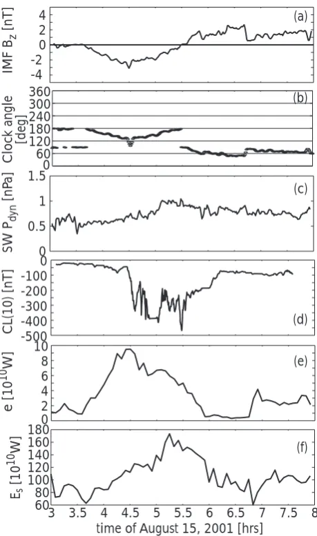
Figure 2 shows the 15 August 2001 substorm observations and the energy transfer rates calculated as above. The solar wind measurements were recorded by the Geotail spacecraft. Panels 2a–c show the IMFBz, IMF clock angle, and the
so-lar wind dynamic pressure. The substorm occurred when the North American sector was in the nightside, therefore, panel 2d presents the auroral electrojet index calculated from the CANOPUS magnetometer array. Ten stations (FCHU, CONT, DAWS, ESKI, GILL, ISLL, MCMU, RANK, RABB, FSIM) were used, from which the minimum of the north component was selected at each time step, yielding theCL index. Panels 2e and 2f show the parameter calculated from the solar wind parameters, and the total energy trans-ferred through the magnetopause surface in the GUMICS-4 MHD simulation using the method described in Palmroth et al. (2003).
Figure 2a shows that the IMFBz was around zero at the
beginning of the simulated time period and turned weakly southward∼03:39 UT. Simultaneously, the IMF clock an-gle (Fig. 2b) rotated into the sector 120◦−180◦. Solar wind dynamic pressure (Fig. 2c) was low, below 1 nPa, during the event. The onset of a modest substorm (∼ −500 nT) occurred at 04:27 UT in the CANOPUS magnetograms (Fig. 2d). Thus, the growth phase of the substorm lasted∼ 48 min, and at substorm onset the IMF was still southward, indicating that the energy input mechanism was still active. Theparameter (Fig. 2e) started to increase when the IMF
603 3.5 4 4.5 5 5.5 6 6.5 7 7.5 8
SW P
dy
n
[nP
a]
Cloc
k angle [deg]
IMF B
z
[nT]
time of August 15, 2001 [hrs] -500
-400 -300 -200 -100 0
CL(10) [nT]
0 2 4 6 8 10
e
[10
10 W]
80 100 120 140 160 180
Es
[10
10 W] -4 -2 0 2 4
0 0.5 1 1.50
60 120 180 240 300 360
(a)
(b)
(c)
(d)
(e)
[image:5.595.313.543.60.449.2](f)
Fig. 2. Solar wind conditions during the 15 August 2001 substorm.
(a) IMFBz, (b) IMF clock angle, (c) solar wind dynamic pressure,
(d)CLindex calculated from CANOPUS magnetometer network, (e), (f) total energy through the magnetopause surface in a global MHD simulation.
Bzturned southward. Theparameter reached a quite
mod-erate peak value of 1·1011W simultaneously with the min-imum of IMFBz. The total energy transferred through the
MHD magnetopause started to increase about a half an hour later than, and increased until the IMF Bz rotated
north-ward.
3
2
1
0 0
3 6 9
GUMICS-4 J
oule Heating [10
11 W]
Ahn et al. [1983] J
oule Heating [10
11
W]
GUMICS-4 2.1.9.108.AE(86) [Ahn et al., 1983]
14 16 18 20 22 24 02 04 06 08
GUMICS-4
2.109(4.4.sqrt(AL(86))-7.6) [Ostgaard et al., 2002]
0 0.5 1 1.5 2 2.5
0 1 2 3 4 5
GUMICS-4 Precipitation[10
11 W]
Ostgaard et al. [2002] Precipitation [10
11
W]
(a)
(b)
Time of April 6, 2000 [hrs]
Fig. 3. (a) Joule heating power and (b) precipitation power in the ionosphere during the April 2000 storm as described by the GUMICS-4 global MHD simulation (thick line). The thin lines are calculated using equations presented in Ahn et al. (1983) and Østgaard et al. (2002).
4 Results
4.1 Ionospheric dissipation
Figures 3a and b present the ionospheric Joule heating power and precipitation power in the April 2000 storm. Thick lines show the Joule heating and the precipitation power calculated from the simulation, whereas thin lines depict the Joule heat-ing and the precipitation power usheat-ing the Ahn et al. (1983) and Østgaard et al. (2002) proxies, respectively. The left vertical axis is for the GUMICS-4 results, whereas the right vertical axis is for the Ahn et al. (1983) and Østgaard et al. (2002) formulas. The Østgaard et al. (2002) method is based on Polar satellite measurements of particle precipitation fit-ted to AE andAL indices, while Ahn et al. (1983) used an empirical method based on ground magnetic field mea-surements to calculate the Joule heating rates and fitted the results toAE andAL indices. The Ahn et al. (1983) and Østgaard et al. (2002) proxies are multiplied by two, to ac-count for ionospheric dissipation in both hemispheres. Note
that the precipitation power computed from the simulation is calculated from 60◦latitude poleward, because latitudes be-low 60◦do not reach the 3.7REshell (the inner boundary of
the magnetospheric domain), and thus there cannot be any magnetospheric precipitation sources below this latitude in the simulation.
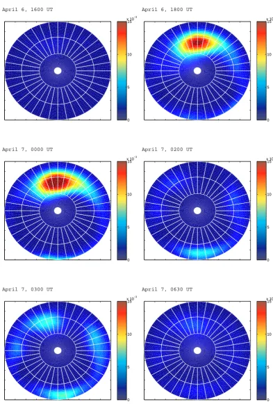
[image:6.595.132.466.63.447.2]April 6, 1600 UT
April 7, 0200 UT
April 7, 0630 UT April 7, 0300 UT
April 6, 1800 UT
[image:7.595.82.501.70.701.2]April 7, 0000 UT
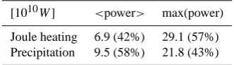
Table 1. Summary of the power dissipated into the ionosphere dur-ing the April 2000 storm.
[1010W] <power> max(power) Joule heating 6.9 (42%) 29.1 (57%) Precipitation 9.5 (58%) 21.8 (43%)
less time variability than the Joule heating power. Table 1 summarises the average and peak values of dissipated Joule heating and precipitation powers, and the relative contribu-tions are also shown.
In Fig. 3a the Joule heating calculated using the Ahn et al. (1983) method does not compare well with the Joule heating calculated from the global MHD simulation. The average level during the storm main phase (∼ 5·1011W) is about ten times larger than the Joule heating rate in the simula-tion. Also, the temporal variation of the two curves are dif-ferent. While the Joule heating in the simulation appears to be correlated with the solar wind dynamic pressure, the Ahn et al. (1983) proxy has (by definition) the shape of theAE in-dex. However, in Fig. 3b the precipitation power calculated from the Østgaard et al. (2002) proxy and the precipitation power calculated from the simulation have similar temporal variation, only the precipitation power in the Østgaard et al. (2002) proxy is two times larger than the precipitation power in the simulation. The Østgaard et al. (2002) proxy starts at a higher level before the storm SSC, otherwise the temporal variation of the two curves are remarkably similar.
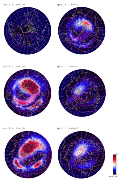
Figure 4 shows the Joule heating color-coded in the sim-ulation during the April 2000 storm in units of Wm−2. The pink lines show the potential isocontours with 10 kV spac-ing. The local noon is at the top, 18:00 MLT to the left, 24:00 MLT at the bottom and 06:00 MLT to the right of each plate. Before the storm SSC (16:00 UT) the ionosphere is quiet. At 18:00 UT during the main phase, the polar cap po-tential difference has increased. Also, the Joule heating is en-hanced, with its maximum clearly on the dayside. Enhanced Joule heating also occurred within the polar cap in the region where the electric field is largest (potential contours are close to each other). Furthermore, there is a faint maximum in the midnight sector along the oval. At 00:00 UT, all regions show much enhanced Joule heating power, and the potential differ-ence has further increased. At 02:00 UT the Joule heating power has decreased with only a small distribution over the polar cap. At 03:00 UT, at the largest peak in the Joule heat-ing power rate durheat-ing the event (durheat-ing the largest pressure pulse), the Joule heating power distribution covers both the dayside and the nightside ovals, as well as regions within the polar cap. At 06:30 UT, near the end of the simulated period, the decreased Joule heating rate is concentrated within the polar cap; the oval shows only faintly.
Figure 5 shows the precipitation power [Wm−2] color-coded at the same moments of time as in Fig. 4. The out-ermost circle is the latitude 60◦ in the ionosphere, and the
[image:8.595.84.250.99.145.2]innermost circle is 88◦in latitude, and MLT sectors are as in Fig. 4. Before the storm (16:00 UT) there is no significant precipitation into the ionosphere. At 18:00 UT, the precipi-tation power has increased with a clear maximum in the day-side in the cusp region. At 00:00 UT the situation has not changed from the previous panel, but at 02:00 UT the day-side maximum has been diminished, and instead, particularly in the nightside and dawn oval, there are clear precipitation power maxima. At 03:00 UT, the precipitation has increased in the oval region, but at 06:30 UT the precipitation power rate has decreased almost to the level preceding the storm.
The total ionospheric dissipation can be compared to the total energy transferred through the magnetopause surface (see Figs. 1 and 2). As can be seen from Fig. 1, the en-ergy input through the magnetopause surface during the main phase of the April 2000 storm is∼25 000 GW, whereas the parameter suggests an energy input of∼5000 GW during the main phase. The ionosphere consumes the total amount of∼190 GW during the main phase, which is less than 1% of the energy transferred through the surface and∼4% of . During the recovery phase, ∼10 000 GW is transferred through the magnetopause surface, and the total amount of ∼170 GW, about 2% of input, is dissipated into the iono-sphere.
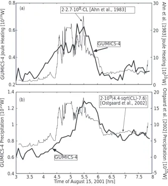
Figure 6 presents the ionospheric Joule heating power and the precipitation power during the 15 August 2001 substorm simulation; the format of the figure is similar to that in Fig. 3. The Joule heating and precipitation powers start to increase around 04:00 UT, reaching their peaks around 05:30 UT. The decreasing phase of the ionospheric dissipation lasts until ∼06:20 UT. Both ionospheric dissipation power rates show an increasing trend during the simulated time period. The peak value of the ionospheric Joule heating rate is about 50% of the precipitation energy peak value. Table 2 summarises the ionospheric dissipation power as average and maximum values; also the relative contributions are shown.
For the substorm simulation case, the temporal variation of the Joule heating and precipitation powers from the Ahn et al. (1983) and the Østgaard et al. (2002) proxies appear to be remarkably similar with the temporal variation of the Joule heating and the precipitation powers calculated from the simulation. Note, however, that the scales between the left and right vertical axes are not the same. The Joule heat-ing in the Ahn et al. (1983) proxy is over thirty times larger than the Joule heating in the simulation. The precipitation in the Østgaard et al. (2002) proxy is about ten times larger than the precipitation power in the simulation. Comparing to Fig. 2, during the 15 August 2001 substorm, on average, 1200 GW is transferred through the magnetopause surface during the substorm, while theparameter indicates about 50 GW energy input on average. The ionosphere consumes only 12 GW, on average (Table 2), which is∼1% of the to-tal transferred energy, and∼24% of the averageduring the substorm.
scal-0 5 10 15 x 10−3
0 5 10 15 x 10−3
0 5 10 15 x 10−3
0 5 10 15 x 10−3
0 5 10 15 x 10−3
0 5 10 15 x 10−3
April 6, 1600 UT April 6, 1800 UT
April 7, 0000 UT April 7, 0200 UT
[image:9.595.96.490.55.637.2]April 7, 0300 UT April 7, 0630 UT
Fig. 5. Precipitation power color-coded in the simulation at six moments of time during the April 2000 storm, units Wm−2.
ing is different. Before the substorm onset (05:00 UT in the simulation) a small amount of Joule heating is concentrated mainly in the nightside oval. At 05:30 UT, after the onset, the Joule heating power rate is enhanced in the nightside oval, and there is a small maximum in the duskside oval. Half an
[image:9.595.101.490.67.235.2]hour later the Joule heating power has already decreased to the level preceding the substorm.
0.2 0.4 0.6 0.8
0 10 20 30
GUMICS-4 J
oule Heating [10
10 W]
Ahn et al. [1983] J
oule Heating [10
10
W]
2.2.7.108.CL [Ahn et al., 1983]
GUMICS-4
3 3.5 4 4.5 5 5.5 6 6.5 7 7.5 8
0.4 0.6 0.8 1 1.2 1.4
-5 0 5 10 15 20
GUMICS-4
2.109(4.4.sqrt(CL)-7.6) [Ostgaard et al., 2002]
Ostgaard et al. [2002] Precipitation [10
10
W]
GUMICS-4 Precipitation [10
10 W]
(a)
(b)
Time of August 15, 2001 [hrs]
[image:10.595.131.466.64.435.2]Fig. 6. (a) Joule heating power and (b) precipitation power in the ionosphere during the 15 August 2001 substorm as described by the GUMICS-4 global MHD simulation (thick line). The thin lines are calculated using equations presented in Ahn et al. (1983) and Østgaard et al. (2002).
Table 2. Summary of the power dissipated into the ionosphere dur-ing the 15 August 2001 substorm.
[109W] <power> max(power) Joule heating 3.6 (29%) 6.5 (33%) Precipitation 8.7 (71%) 12.9 (67%)
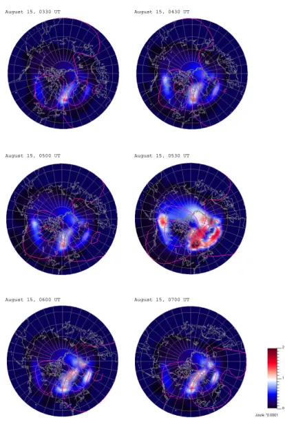
color scaling. Before the substorm onset there is already a small amount of precipitation centered approximately at the 21:00 MLT sector, and a smaller maximum exists approx-imately at the 02:00 MLT sector. After the onset the pre-cipitation maximum at the 21:00 MLT sector is enhanced, persisting still at 06:00 UT. At 07:00 UT the precipitation power has recovered to the level preceding the substorm. The 02:00 MLT maximum remains approximately the same in size throughout the simulated period.
4.2 Joule heating power distribution in the ionosphere Figure 9 presents the ionospheric Joule heating rates dis-tributed at different longitudes and latitudes during the April 2000 storm simulation: Figs. 9a–c show the Joule heating rates in the dayside, dawn and dusk sectors, and in the night-side, respectively. Figures 9d–f show the Joule heating rates at low latitudes, within the auroral oval, and within the polar cap, respectively. As is evident from Fig. 9, the SSC is visi-ble at all local times and latitudes simultaneously around the ionosphere. The temporal variation of the different curves are similar, indicating that all the peaks and valleys in the Joule heating power occur at the same time. However, Fig. 9 also shows that the location contributing mostly to the Joule heating rate during the storm evolution is the dayside oval and low latitudes. For instance, the nightside Joule heating rate is about 40% of the dayside Joule heating rate.
[image:10.595.84.251.539.583.2]August 15, 0330 UT
August 15, 0700 UT August 15, 0600 UT
August 15, 0530 UT August 15, 0500 UT
[image:11.595.86.501.78.696.2]August 15, 0430 UT
2 4 6 8 10 12 14 x 10−4
2 4 6 8 10 12 14 x 10−4
2 4 6 8 10 12 14 x 10−4
2 4 6 8 10 12 14 x 10−4
2 4 6 8 10 12 14 x 10−4
2 4 6 8 10 12 14 x 10−4
August 15, 0330 UT August 15, 0430 UT
August 15, 0500 UT August 15, 0530 UT
[image:12.595.98.494.61.637.2]August 15, 0600 UT August 15, 0700 UT
Fig. 8. Precipitation power color-coded in the simulation at six moments of time during the August 2001 substorm, units Wm−2.
area, and in the polar cap, respectively. Contrary to the storm event, in the substorm case most of the Joule heating power is concentrated to the oval latitudes. The Joule heating power in the nightside exceeds the Joule heating power in the dawn and dusk and in the dayside.
4.3 Precipitation power distribution in the ionosphere
[image:12.595.102.494.67.235.2]0 5 10 150 5 10 150 5 10 15 JH po wer [10 10W]
Night 20-04 MLT Dawn&Dusk 04-08 & 16-20 MLT Day 08-16 MLT
JH po wer [10 10W] JH po wer [10 10W] 0 5 10
14 16 18 20 22 24 02 04 06 08 0 5 10 JH po wer [10 10 W]
time of April 6, 2000 [hrs] Polar cap 75°-88°
Oval 60°-75° JH po wer [10 10 W] 0 5
10 Low latitude0°-60°
[image:13.595.311.541.62.460.2]JH po wer [10 10 W] (a) (b) (c) (d) (e) (f)
Fig. 9. Joule heating power during the April 2000 storm in (a) the dayside 08:00–16:00 MLT, (b) dawn 04:00–08:00 MLT and dusk 16:00–20:00 MLT, (c) nightside 20:00–04:00 MLT, (d) low lati-tudes 0◦–60◦, (e) oval latitudes 60◦–75◦, (f) polar cap latitudes 75◦–88◦. Both hemispheres are present in panels.
e) in the April 2000 storm simulation. Figure 11 clearly illus-trates that the major part of precipitation power is dissipated in the dayside oval and cusp regions during the April 2000 storm simulation.
Figure 12 shows the precipitation power distributed over latitude and longitude during the 15 August 2001 substorm simulation. Figures 12a–c show the precipitation powers in the dayside, dawn and dusk sectors, and in the nightside, whereas Figs. 12d and e depict the precipitation powers in the oval and polar cap areas, plotted in the same scale. Fig-ure 12 demonstrates that during the substorm, a major part of the precipitation power comes from the nightside oval. The dawn and dusk precipitation peak value reaches∼80% of the nightside precipitation peak value.
0 1 2 3 0 1 2 3 4
3 3.5 4 4.5 5 5.5 6 6.5 7 7.5 8 0
1 2 3 4
time of August 15, 2001 [hrs] 0
1 2 3
Day 08-16 MLT
JH po
wer
[10
9 W]
Polar cap 75°-88° Oval 60°-75° JH po wer [10 9 W] JH po wer [10 9 W]
Night 20-04 MLT Dawn&Dusk 04-08 & 16-20 MLT
JH po wer [10 9 W] JH po wer [10 9W] 0 1 2 3 0 1 2 3 4 JH po wer [10 9 W] Low latitude 0°-60° (a) (b) (c) (d) (e) (f)
Fig. 10. Joule heating power during the 15 August 2001 substorm in the (a) dayside 08:00–16:00 MLT, (b) dawn 04:00–08:00 MLT and dusk 16:00–20:00 MLT, (c) nightside 20:00–04:00 MLT, (d) low latitudes 0◦–60◦, (e) oval latitudes 60◦–75◦, and (f) polar cap latitudes 75◦–88◦. Both hemispheres are present in panels.
4.4 Relation between input and output
After calculating the ionospheric dissipation directly from the simulation of the two events, we set out to search for a formulation of the ionospheric dissipation as a function of the solar wind parameters. Ideally one would like to find a general formulation, which gives the same functional de-pendence on the solar wind parameters for both simulated events, implying that it may be valid also in a more general case. The parameters to be considered include at least the so-lar wind densityρ, velocityvand the IMFBz. We chose the
simplest power law function for fitting the simulation data, i.e.
Pionosphere =C
ρ
ρ0
av
v0
b"
exp pBz,I MF 2µ0pdyn
!#d
[image:13.595.51.279.74.460.2]0 0.5 1 1.5 2 0 0.5 1 1.5 0 0.5 1 1.5 0 0.5 1 1.5
14 16 18 20 22 24 02 04 06 08 0
0.5 1 1.5
time of April 6, 2000 [hrs] Polar cap 75°-88°
Oval 60°-75° Night 20-04 MLT Dawn&Dusk 04-08 & 16-20 MLT Day 08-16 MLT
[image:14.595.316.542.66.396.2]Prec. po wer [10 11 W] Prec. po wer [10 11 W] Prec. po wer [10 11 W] Prec. po wer [10 11 W] Prec. po wer [10 11 W] (a) (b) (c) (d) (e)
Fig. 11. Precipitation energy during the April 2000 storm in (a) the dayside 08:00–16:00 MLT, (b) dawn 04:00–08:00 MLT and dusk 16:00–20:00 MLT, (c) nightside 20:00–04:00 MLT, (d) oval latitudes 60◦–75◦, and (e) polar cap latitudes 75◦–88◦. Both hemi-spheres are present in panels.
where ρ0 = mp ·7.3·106m−3 = 1.22 ·10−20kgm−3 and
v0 =400 km/s are chosen as typical solar wind density and velocity; this is for convenience to obtain a correct unit for the power law. C is thus a constant having units of Watts. Because we want to have the power law formula positive and monotonically increasing as a function of negative IMF Bz, we model the IMFBz inside an exponential.
Further-more, the IMFBz is scaled in the power law by the
magne-topause magnetic field given by the pressure balance equa-tion. Table 3 shows the fitted coefficientsC, a, b, and d, together with their error margins and correlation coefficients with the simulation results. Three fits were made: output
Pionospheretaken to be only the Joule heating, only
precipita-tion, and for the sum of Joule heating and precipitation. The first block presents the fitted coefficients, as well as coeffi-cients calculated from the scaling law theory in Sect. 2.3, for Joule heating power in the two events. Comparison of the fitted and theoretical values indicates clearly that the simu-lated Joule heating power fitted to the solar wind data gives larger values for a andb in both events compared to what
3 3.5 4 4.5 5 5.5 6 6.5 7 7.5 8 time of August 15, 2001 [hrs]
Night 20-04 MLT Dawn&Dusk 04-08 & 16-20 MLT Day 08-16 MLT
Precipitation power [10
9 W] Polar cap 75°-88° Oval 60°-75°
Precipitation power [10
9 W]
Precipitation power [10
9W]
Precipitation power [10
9 W]
Precipitation power [10
9 W] 0 2 4 6 0 2 4 6 0 2 4 6 0 5 10 0 5 10 (a) (b) (c) (d) (e)
Fig. 12. Precipitation power during the 15 August 2001 substorm in the (a) dayside 08:00–16:00 MLT, (b) dawn 04:00–08:00 MLT and dusk 16:00–20:00 MLT, (c) nightside 20:00–04:00 MLT, (d) oval latitudes 60◦–75◦, and (e) polar cap latitudes 75◦–88◦. Both hemispheres are present in panels.
would be expected from the scaling law theory in Sect. 2.3. In both events,ais roughly the same, but in the April storm simulationbis larger than in the August substorm simulation by a factor of 1.6. This suggests that the solar wind density has roughly the same influence on the deposited Joule heat-ing power, but in the April storm simulation the solar wind speed has much more influence on the deposited Joule heat-ing power than in the August substorm event. However, the coefficientd should be negative, because the Joule heating rate should increase with increasing negative IMFBz. As can
[image:14.595.51.286.71.402.2]0 50 100 150 200 250 0
1 2 3 4
3 3.5 4 4.5 5 5.5 6 6.5 7 7.5 8
6 8 10 12 14 16 18 20
total JH + precipitation power fitted power law
correlation 0.83
time of August 15, 2001 [hrs]
14 16 18 20 22 24 26 28 30 32
0 1 2 3 4
10
11
W
total JH + precipitation power fitted power law
correlation 0.88
time of April 6, 2000 [hrs]
10
9 W
10
11
W
data points total JH + precipitation power
fitted power law correlation 0.94
(a)
(b)
(c)
August
[image:15.595.108.489.65.446.2]substorm
April storm
Fig. 13. Sum of Joule heating and precipitation powers (thick line) and fitted curve from Eq. (10) (thin line) for (a) 15 August 2001 substorm simulation, (b) 6 April 2000 storm simulation, and (c) both events merged to the same data vector. Note the different horizontal axis.
The second block of Table 3 presents the results for fitting the solar wind data into the precipitation power calculated in the simulation. The scaling law theory in Sect. 2.3 now pre-dicts a largerathan is obtained by fitting the solar wind data into the precipitation in the simulation. In the August sub-storm simulationais comparable in size withain the April storm simulation. The coefficientbis comparable in size in both events, it is also roughly the same as what the scaling law theory predicts. Curiously, now the coefficientd is neg-ative in the April storm simulation and positive in the Au-gust substorm simulation, indicating that the IMF direction would have influence on the deposited precipitation power during the April storm, but during the August substorm the deposited precipitation would be almost independent of the IMF direction. Note, however, that the error estimate is large for the positived coefficient in the substorm case. In both events, the precipitation power calculated using Eq. (10) is well-correlated to what is calculated in the simulation, the correlation coefficient being 0.86 for both events.
con-tributing pieces (precipitation and Joule heating) separately; also the obtained exponents are closer to the scaling law pre-dictions.
5 Summary and discussion
In this paper we have calculated the power dissipated into the ionosphere in a global MHD simulation during two events, a magnetic storm and a magnetospheric substorm. We have studied the latitudinal and longitudinal distribution of the ionospheric dissipation from two parameters, the Joule heat-ing and the particle precipitation. Furthermore, we have compared the results to empirical proxies of the Joule heating and precipitation powers. Finally, we have obtained a power law which predicts the total power deposited into the iono-sphere from the solar wind parameters with high correlation between the actual simulation results.
Lu et al. (1998) calculated the Joule heating and precip-itation powers during a magnetic storm using the AMIE technique. They obtained a globally integrated average of 190 GW for Joule heating, and about 90 GW for particle pre-cipitation during a 2-day storm period in January 1997. Com-pared to our results in Fig. 3 and Table 1, the Joule heating in the MHD simulation consumes less than 100 GW, with precipitation about 100 GW in both hemispheres during the storm. Therefore, the MHD simulation produces less Joule heating than the AMIE technique, even though the storm modeled in Lu et al. (1998) (Dst peak−85 nT) was much
smaller than the April 2000 storm. Precipitation in the sim-ulation deposits roughly the same amount of power as that obtained from the AMIE technique. Furthermore, in the Lu et al. (1998) analysis, the peaks in the Joule heating and the precipitation powers are reached at a time when there is a sudden change in the dynamic pressure during the southward IMF period. In the MHD simulation, the peak in the precip-itation power occurred during the main phase and southward IMF, also as a response to a solar wind pressure pulse. The peak in the Joule heating power, however, occurs during the largest dynamic pressure pulse, which took place during the storm recovery phase and northward IMF. A closer examina-tion of the simulaexamina-tion results around 03:00 UT (the time of the maximum Joule heating) reveals that at that time an inter-hemispherical current system, presumably the result of dif-ferent conductivities between the two hemispheres, develops in the simulation. Such a current system, is likely to cause a large amount of Joule heat, because in an interhemispherical current system the current closes over a large distance from the one hemisphere to another. This somewhat unexpected result warrants further study.
The Joule heating power calculated from the MHD simula-tion is clearly different from the empirical proxy by Ahn et al. (1983) in the April 2000 storm event. The temporal variation of the Joule heating power in the MHD simulation resembles remarkably the temporal variation of the solar wind dynamic pressure, whereas the Joule heating power in the Ahn et al. (1983) formula is a scaledAEindex. Janhunen and
Koski-nen (1997) reported that in the GUMICS-3 MHD simulation (earlier version of GUMICS-4) the Region 1 current system largely closes into the dayside magnetopause currents, which are known to be modified by the solar wind dynamic pres-sure. Furthermore, the temporal variation of the field-aligned currents in GUMICS-4 (not shown) also resembles the tem-poral variation of the solar wind dynamic pressure. There-fore, it is natural that the Joule heating power, which de-pends on the square of the field-aligned currents, also follows the solar wind dynamic pressure variations in the GUMICS-4 MHD simulation. The closure of Region 1 currents to mag-netopause currents was also noticed by Siscoe et al. (2002).
The temporal variation of the calculated precipitation power during both events, as well as the temporal variation of Joule heating power during the substorm event, is well-correlated with the temporal variation of the empirical prox-ies of Østgaard et al. (2002) and Ahn et al. (1983). However, the amount of energy deposited into the ionosphere in the simulation is much smaller than the power deposited into the ionosphere in the empirical proxies. The Joule heating power deposited during the storm simulation is 25% of the Joule heating power given by the Ahn et al. (1983) formula. The precipitation power deposited into the ionosphere is about 50% of the precipitation power using the Østgaard et al. (2002) formula. The situation is worse in the substorm sim-ulation. The amount of Joule heating power deposited into the ionosphere in the simulation is only 4% of the amount of Joule heating power according to the Ahn et al. (1983) for-mula. The amount of precipitation power is about 10% of the amount of precipitation power according to the Østgaard et al. (2002) formula.
The April 2000 storm was so intense that the oval was lo-cated further equatorward than is usual, which means that part of the oval was equatorward of the ionospheric mapping of the inner boundary of the GUMICS-4 MHD simulation (3.7RE). Therefore, a major part of nightside precipitation
Table 3. Power law fittings.
C [GW] a b d corr.
Scaling law 0.67 1.33 JH
April 4.5·(1±0.09) 1.21±0.08 3.90±0.33 0.57±0.38 0.76 JH August 11·(1±0.24) 1.17±0.21 2.32±0.67 -6.05±0.77 0.83 JH
Scaling law 1.17 3.33 Prec.
April 20·(1±0.06) 0.36±0.05 3.03±0.22 -3.31±0.25 0.86 Prec. August 15·(1±0.15) 0.68±0.13 3.21±0.41 0.10±0.47 0.86 Prec.
Scaling law* 0.88 2.11 JH+Prec.
April 26·(1±0.05) 0.75±0.04 2.89±0.18 -1.76±0.21 0.88 JH+Prec. August 25·(1±0.17) 0.82±0.14 3.03±0.47 -1.75±0.53 0.83 JH+Prec.
Both events 25·(1±0.03) 0.80±0.03 2.87±0.16 -1.81±0.18 0.94 JH+Prec.
∗Geometric mean of Joule heating and precipitation power scaling exponents.
Practically all studies concerning the ionospheric dissipa-tion have reached the conclusion that Joule heating deposits more energy than precipitation (e.g. Lu et al., 1998). Our result shows that in both events the precipitation deposits, on average, slightly more energy than the Joule heating. The underestimation of Joule heating in GUMICS-4 is a con-sequence of several different sources, one of which can be the typically 20–30% lower polar cap potentials as compared to, for example, SuperDARN results. As the Joule heating is given by6PE2, underestimation of the polar cap
poten-tial by 30% leads to underestimation in the Joule heating by ∼50%. For example, during the April 2000 storm, the aver-age polar cap potential during the main phase according to SuperDARN was about 80 kV, whereas the GUMICS-4 re-sult was about 50 kV, giving 2.56 for the ratio of polar cap potentials squared. The Joule heating rate during the April 2000 storm main phase multiplied by 2.56 gives∼2·1011W, which is now of the same order of magnitude as the Ahn et al. (1983) value (Fig. 3). Similarly, during the 15 August 2001 substorm event, the polar cap potential was steadily about 50 kV (McPherron et al., 2002), whereas GUMICS yielded about 30 kV. Again, the ratio of polar cap potentials squared gives 2.8, and Joule heating multiplied by this value during the substorm is about 1.5·1010W, which is still less than that given by Ahn et al. (1983), but of the same order of magni-tude.
An additional effect causing the low Joule heating values could be caused by a more localized field-aligned current clo-sure. As a simplified thought experiment, let us consider a single current loop that closes through the ionosphere, i.e. a loop where the acceleration region in the magnetosphere and the ionospheric load are connected in a series. The power consumed in a current loop is determined by the potential difference and the total current (P =U I). In a single cur-rent loop the same curcur-rent flows through the acceleration re-gion and the ionospheric load, and, therefore,Paccel/Uaccel=
Pionosph/Uionosph. The characteristic energy of precipitating
electrons determines thatPaccel=PprecandPionosph=PJ H,
we obtainPprec/PJ H =Uaccel/Uiono. In both simulated cases
Pprec/PJ H>1, which means thatUaccel/Uiono>1, indicat-ing that the potential difference in the ionosphere is smaller than in the acceleration region, suggesting that the current closes over a relatively short distance in the ionosphere. Therefore, the fact that Joule heating is a smaller energy sink than precipitation in the global MHD simulation might in-dicate that in the simulation the currents could close over a short distance in the ionosphere. Satellite observations re-ported by Marklund et al. (1998) demonstrate that the clo-sure of a part of the field-aligned currents in the substorm current wedge occurs locally near the surge head. Further-more, a small error in the GUMICS-4 total Joule heating re-sult can also be caused by the limited ionospheric grid reso-lution. For example, discrete intensive arcs with sizes below the GUMICS-4 ionospheric grid resolution produce locally high values of Joule heating. We estimate roughly that the discrete arcs can increase the total Joule heating up to 10%.
When comparing the latitudinal and longitudinal distri-butions of the ionospheric dissipation in the two simulated events the differences between the storm and substorm cases become evident. In short, the dayside has a dominant role in the storm case, whereas the nightside oval dissipates most of the power in the substorm case. Another clear distinc-tion can be seen in the Tables 1 and 2. While in the storm case the Joule heating and the precipitation dissipate roughly the same amount of energy into the ionosphere, during the substorm precipitation energy exceeds that of Joule heating. This can partly be explained by the fact that a large part of the precipitation is not included in the storm simulation, due to the 3.7REinner boundary of the magnetospheric domain,
sum of Joule heating and precipitation power, which is natu-ral as the two parameters are not independent of each other. The relative importance of the exponentsa,b, anddsuggests that the solar wind density and velocity have more impact on the total ionospheric dissipation than the IMFBz. This
may not be universally true. Coincidentally, in the two cho-sen events the impact of the solar wind pressure was stronger than the IMF. In the April 2000 storm the solar wind dynamic pressure was unusually high, and in the moderate August 2001 substorm the IMFBzwas quite weak and not rapidly
varying. This suggests that more events with different inputs must be simulated, to obtain a power law that would recover the earlier empirically strong correlation found between en-ergy dissipation and IMFBz.
Acknowledgements. We thank the NSSDC for maintaining the
CDAWeb facility through which Geotail data for the simulation input were obtained. The CANOPUS instrument array was con-structed and is maintained and operated by the Canadian Space Agency for the Canadian scientific community. The work of M. P. and P. J. is supported by the MaDaMe program of the Academy of Finland.
The Editor in Chief thanks M. Wiltberger and another referee for their help in evaluating this paper.
References
Akasofu, S.-I.: Energy coupling between the solar wind and the magnetosphere, Space Sci. Rev., 28, 121–190, 1981.
Acu˜na, M. H., Ogilivie, K. W., Baker, D. N., Curtis, S. A., Fairfield, D. H., and Mish, W. H.: The global geospace science program and its investigations, Space Sci. Rev., 71, 5–21, 1995.
Ahn, B.-H. J., Akasofu, S. -I., and Kamide, Y.: The Joule heat pro-duction rate and the particle energy injection rate as function of the geomagnetic indicesAEandAL, J. Geophys. Res., 88, 6275–6287, 1983.
Axford, W. I. and Hines, C. O.: A unifying theory of high-latitude geophysical phenomena and geomagnetic storms, Can. J. Phys., 39, 1433, 1961.
Dungey, J. W.: Interplanetary magnetic field and the auroral zones, Phys. Rev. Lett., 6, 47-48, 1961.
Huttunen, K. E. J., Koskinen, H. E. J., Pulkkinen, T. I., Pulkkinen, A., Palmroth, M., Reeves, G. D., and Singer, H. J.: April 2000 magnetic storm: Solar wind driver and magnetospheric response, J. Geophys. Res., 107, doi:10.1029/2001JA009154, 2002. Janhunen, P.: GUMICS-3–A global ionosphere-magnetosphere
coupling simulation with high ionospheric resolution, in: Proc. Environmental Modelling for Space-Based Applications, Sept. 18-20 1996 (ESTEC, The Netherlands, ESA SP-392,) 1996. Janhunen, P. and Koskinen, H. E. J.: The closure of Region-1
field-aligned current in MHD simulation, Geophys. Re. Lett., 24, 1419–1422, 1997.
Janhunen, P. and Olsson, A.: The current-voltage relationship re-visited: exact and approximate formulas with almost general va-lidity for hot magnetospheric electrons for bi-Maxwellian and kappa distributions, Ann. Geophysicae, 16, 292–297, 1998. Lu, G., Baker, D N., McPherron, R. L., Farrugia, C. J,
Lum-merzheim, D., Ruohoniemi, J. M., Rich, F. J., Evans, D. S., Lepping, R. P., Brittnacher, M., Li, X., Greenwald, R., Sofko, G., Villain, J., Lester, M., Thayer, J., Moretto, T., Milling, D.,
Troshichev, O., Zaitzev, A., Odintzov, V., Makarov, G., and Hayashi, K.: Global energy deposition during the January 1997 magnetic cloud event, J. Geophys. Res., 103, 11 685–11 694, 1998.
Marklund, G. T., Karlsson, T., Blomberg, L. G., Lindqvist, P.-A., F¨althammar, C.-G., Johnson, M. L., Murphree, J. S., Andersson, L., Eliasson, L., Opgenoorth, H. J., and Zanetti, L. J.: Observa-tions of the electric field fine structure associated with the west-ward traveling surge and large-scale auroral spirals, J. Geophys. Res., 103, 4125–4144, 1998.
McPherron, R. L., Kivelson, M. G., Khurana, K., Amm, O., Baker, J. B., Balogh, A., R`eme, H., Connors, M., Creutzberg, F., Dan-douras, I., Mann, I., Milling, D., Moldwin, M. B., Rostoker, G., Russell, C. T., and Singer, H.: Cluster observations of the post-midnight plasma sheet at 18 Re during substorms, in: Proceed-ings of the Sixth International Conference on Substorms, edited by Winglee, R. M., University of Washington, Seattle, USA, March 25-29, 283–290, 2002.
Newell, P. T., Lyons, K. M., and Meng, C.-I.: A large survey of electron acceleration events, J. Geophys. Res., 101, 2599–2614, 1996.
Østgaard, N. R., Vondrak, R., Gjerloev, J. W., and Germany, G. A.: A relation between the energy deposition by electron precipita-tion and geomagnetic indices during substorms, J. Geophys. Res. 107(A9), 1246, doi: 10.1029/2001JA002003, 2002..
Palmroth, M., Janhunen, P., Pulkkinen, T. I., and Peterson, W. K.: Cusp and magnetopause locations in global MHD simulation, J. Geophys. Res., 106, 29 435–29 450, 2001.
Palmroth, M., Pulkkinen, T. I., Janhunen, P., and Wu, C. C.: Storm-time energy transfer in global MHD simulation, J. Geophys. Res., 108(A1), 1048, doi:10.1029/2002JA009446, 2003. Papadopoulos, K., Goodrich, C., Wiltberger, M., Lopez, R., and
Lyon, J. G.: The physics of substorms as revealed by the ISTP, Phys. Chem. Earth (c), 24, 189–202, 1999.
Pulkkinen, T. I., Ganushkina, N. Yu., Tanskanen, E. I., Lu, G., Baker, D. N., Turner, N. E., Fritz, T. A., Fennell, J. F., and Roeder, J.: Energy dissipation during a geomagnetic storm: May 1998, Adv. Space Res., 30, 2231–2240, 2002.
Robinson, R. M., Vondrak, R. R., Miller, K., Dabbs, T., and Hardy, D.: On calculating ionospheric conductances from he flux and energy of precipitating electrons, J. Geophys. Res., 92, 2565– 2569, 1987.
Richmond, A. D. and Kamide, Y.: Mapping electrodynamic fea-tures of the high-latitude ionosphere from localized observations-Technique, J. Geophys. Res., 93, 5741–5759, 1988.
Scurry, L. and Russell, C. T.: Proxy studies of energy trasnfer to the magnetosphere, J. Geophys. Res., 96, 9541–9548, 1991. Siscoe, G. L., Crooker, N. U., and Siebert, K. D.:
Transpo-lar potential saturation: Roles of Region 1 current system and solar wind ram pressure, J. Geophys. Res., 107(A10), 1321, doi:10.1029/2001JA009176, 2002.
Turner, N. E., Baker, D. N., Pulkkinen, T. I., Roeder, J. L., Fennell, J. F., and Jordanova, V. K.: Energy content in the storm time ring current, J. Geophys. Res., 106, 19 149–19 156, 2001.
Walker, R. J., Ogino, T., Raeder, J., and Ashour-Abdalla, M.: A global magnetohydrodynamic simulation of the magnetosphere when the interplanetary magnetic field is southward: The on-set of magnetotail reconnection, J. Geophys. Res., 98, 17 235– 17 249, 1993.