Int. J. Climatol.(2012)
Published online in Wiley Online Library (wileyonlinelibrary.com) DOI: 10.1002/joc.3530
A daily homogenized temperature data set for Australia
Blair Trewin*
National Climate Centre, Australian Bureau of Meteorology, Melbourne, VIC, Australia
ABSTRACT:A new homogenized daily maximum and minimum temperature data set, the Australian Climate Observations Reference Network – Surface Air Temperature data set, has been developed for Australia. This data set contains data from 112 locations across Australia, and extends from 1910 to the present, with 60 locations having data for the full post-1910 period.
These data have been comprehensively analysed for inhomogeneities and data errors ensuring a set of station temperature data which are suitable for the analysis of climate variability and trends. For the purposes of merging station series and correcting inhomogeneities, the data set has been developed using a technique, the percentile-matching (PM) algorithm, which applies differing adjustments to daily data depending on their position in the frequency distribution. This method is intended to produce data sets that are homogeneous for higher-order statistical properties, such as variance and the frequency of extremes, as well as for mean values. The PM algorithm is evaluated and found to have clear advantages over adjustments based on monthly means, particularly in the homogenization of temperature extremes. Copyright2012 Royal Meteorological Society
KEY WORDS temperature data; Australia; homogenization
Received 9 January 2012; Revised 14 May 2012; Accepted 16 May 2012
1. Introduction
High-quality temperature data sets are vital for climate monitoring, and especially the monitoring of climate change. Many temperature data sets exist at the global (Hansen et al., 1999, 2001; Brohan et al., 2006; Smith
et al., 2008), regional (Klein Tank et al., 2002) and national scales.
If a temperature data set is to be used for monitoring climate change it is important that it be homogeneous; that is, changes in the temperature as shown in the data set reflect changes in the climate, and not changes in the external (non-climatic) conditions under which the observations are made. Potential non-climatic influences on temperature observations, which are discussed in more depth in sources such as Petersonet al. (1998), Aguilar
et al. (2003) and Trewin (2010), include changes in local ground conditions around an observation site, changes in instruments and changes in observation procedures. In addition, many station ‘series’ are taken from more than one location, despite often appearing under a single geographical name.
Very few century-scale temperature station series are totally free of such influences, and thus careful homoge-nization is required in order to produce a homogeneous data set. Whilst site-specific inhomogeneities have only a marginal impact on observed temperature trends at the global scale (Jones and Wigley, 2010), they can have a
∗Correspondence to: B. Trewin, National Climate Centre, Australian Bureau of Meteorology, Melbourne, VIC, Australia.
E-mail: [email protected]
much more substantial effect on outcomes at the local and regional scale.
The homogenization process is a two-stage process: firstly the detection of inhomogeneities in the data and secondly the adjustment of data to remove those inhomogeneities. The detection of inhomogeneities at the annual and monthly is a well-explored problem, both in climate science and in the broader statistical literature. Reviews on this topic include those of Peterson et al. (1998) and Reeveset al. (2007), although there have been more recent developments, such as Li and Lund (2012) and Toretiet al. (2012).
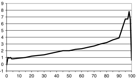
Adjustment procedures have received much less atten-tion, with most data sets applying adjustments on the basis of annual (Della-Marta et al., 2004) or monthly (Joneset al., 1986; Begertet al., 2005) means. However, homogenization of mean temperatures does not neces-sarily imply homogenization of higher-order statistical properties such as variance, or derived statistics which are a function of those higher-order properties, such as the occurrence of extremes. This issue was initially iden-tified by Trewin and Trevitt (1996), who found that in some cases an inhomogeneity, such as a site move, affected different parts of the frequency distribution of daily temperature in different ways. This is illustrated by the example shown in Figure 1.
-1 0 1 2 3 4 5 6 7 8 9
0 10 20 30 40 50 60 70 80 90 100
Figure 1. Differences (°C) between percentile points of summer maximum temperature at Albany airport (009741) and Albany town (009500) during the overlap period (2002–2009). The 0th and 100th percentiles indicate the lowest and highest values recorded during the
overlap period.
the results of a benchmarking of numerous homogeniza-tion methods, carried out as part of that project, were reported in the studies of Venemaet al. (2012).
Most national and international data sets which have been homogeneity-adjusted use adjustments calculated on the basis of annual or monthly means. In most cases these apply a uniform adjustment for each calendar month or across the year, although there have been some data sets (some of which use the term ‘daily homogenization’) which apply a different adjustment for each calendar date, normally derived from monthly data (Vincentet al., 2002; Brunetet al., 2006). Whilst a number of techniques have been developed, as described later in this article, to adjust data at the daily time scale using adjustments which are different for different parts of the frequency distribution, or are otherwise dependent on weather types, the only previous known application of such techniques to a large network in a year-round national-level data set is the 1957–1996 Australian daily data set (Trewin, 2001).
This article describes the methodology used for the construction of a new data set, the Australian Climate Observations Reference Network – Surface Air Temper-ature (ACORN-SAT) data set. This data set makes use of substantial recently digitized data (from paper records) to allow homogeneous maximum and minimum temper-ature data to be produced at the daily time scale for the period from 1910 to the present, with coverage across the Australian continent. Documentation and traceability of the data and adjustments at all stages, an increasing priority as described by Thorneet al. (2011), are also a high priority in the ACORN-SAT data set.
2. Data and metadata availability
2.1. Australian network coverage
Temperature observations have been made in Australia since the days of initial European settlement in the late 18th century (Gergis et al., 2009). Various short-term observations (data sets of a few years or shorter) were made up until the middle of the 19th century.
From the 1850s onwards, more systematic observations began to be made across Australia. The longest currently available ‘continuous’ temperature record in Australia commenced in the city of Melbourne in 1855, and by the early 1860s a number of additional stations existed in New South Wales, Victoria and South Australia. The number of stations increased steadily over time, and there was reasonable coverage of the eastern mainland by 1890. Progress was slower in Tasmania and Western Australia, where there were very limited observations outside Hobart and Perth before 1900.
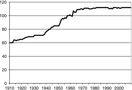
The creation of the Bureau of Meteorology in Jan-uary 1908 brought all meteorological observations under federal government control. This resulted, within a short time, in the implementation of common standards for observations and instrumentation (discussed in more detail below). It also resulted in a rapid increase in the number of stations taking observations. The number of stations then stabilized through most of the 1910–1940 period, before increasing further from 1940 through the early 1950s, initially as a result of the Second World War, then the growth of civil aviation. There have not been dramatic changes in the number of stations since then, although the spread of stations over Australia has become more comprehensive, with observations beginning in the 1950s and 1960s in a number of strategic locations in remote parts of central and northern Australia. Coverage of high-altitude areas in southeastern Australia has also improved greatly in the last 20 years.
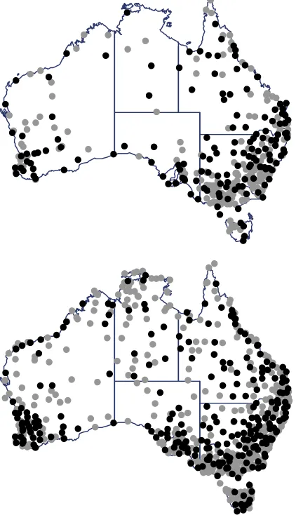
Figure 2 shows the networks in 1930 and 2010, while a summary of the number of stations is shown in Figure 3. The distribution of stations is uneven over Australia (Figure 2), with stations most heavily concentrated in the more densely populated parts of southeastern and south-western Australia. Elsewhere many stations are more than 100 km from their nearest neighbour, with two ACORN-SAT stations (Giles and Rabbit Flat) more than 200 km from their nearest neighbour, and substantial areas in the western and eastern interior have no observations at all.
2.2. Elements available and data digitization
Nearly all stations which measure temperature, with some very limited historical exceptions (almost all pre-1900), observe daily maximum and minimum temperature. They also observe temperatures at a variety of fixed hours. Manual stations make from one (normally 0900 local time) to eight (0000, 0300, . . ., 2100) observations per day, with the majority making observations at 0900 and 1500. Most automatic weather stations (AWSs) have data at 30- or 60 min resolution (as do a few major city stations prior to automation), and an increasing number has data at 1 min temporal resolution. The fixed-hour temperatures do not form part of the ACORN-SAT data set but support the quality-control checks described later in this article, as do other elements such as terrestrial minimum temperature, where available.
Figure 2. The Australian temperature observing network in 1930 (top) and 2010 (bottom). Stations with 40 or more years of data are shown in black. This figure is available in colour online at
wileyonlinelibrary.com/journal/joc
0 200 400 600 800 1000 1200 1400 1600 1800
0 10 20 30 40 50 60 70 80 90 100
Figure 3. Number of Australian temperature stations with at leastN years of digitized daily temperature data. The number of stations, which
are currently open, is shown in black.
prior to 1957 or fixed-hour data (except at 0900 or 1500) prior to 1987, with most data prior to that date available only on paper manuscripts. In contrast, monthly data, which underlie the data set of Della-Martaet al. (2004),
have been almost entirely digitized for some time, which is why the earlier high-quality data sets for Australia focused on the annual or monthly time scale.
In the last decade, there has been an ongoing effort to digitize pre-1957 daily temperature data as part of the CLIMARC project (Clarksonet al., 2001) and associated projects, although large quantities of daily temperature data remain undigitized. Some newly digitized data have not yet undergone any Bureau of Meteorology quality control and are yet to be incorporated into the main Bureau database; these data were used in ACORN-SAT but with particular care.
2.3. Availability of metadata
Metadata – that is, information about the way in which the data have been observed – are important in docu-menting non-climatic influences which can affect tem-perature measurements. These include issues which are specific to individual sites (such as site relocations, instru-ment changes or changes in local site conditions), or issues which affect large parts of the observing network (such as changes in observation times).
The major sources of site-specific metadata available for the ACORN-SAT stations are a digital metadata database (SitesDB) for post-1997 material (and some limited pre-1997 information) and hard-copy station files and instrument registers for pre-1997 material. Major items of relevance for the ACORN-SAT project include:
• Details of site relocations.
• Station inspection reports, including site photographs (or in some earlier periods, sketches) and diagrams. In recent decades, these have been approximately annual at ACORN-SAT stations (although there are a few notable exceptions, particularly at locations which are difficult to access). In the historical data they are much less frequent, with inspection reports often a decade or more apart prior to 1960.
• Changes in instruments. These are perhaps the best-documented changes historically, in part because they involved the expenditure of public funds.
• Instrument tolerance checks carried out at individual sites.
with the project. It is likely that other such changes have occurred historically but without any documentary evidence.
Other information from third parties can also be con-sidered as metadata. This includes maps (particularly topographic maps), and population data, from the Aus-tralian Bureau of Statistics, for urban centres near observ-ing sites.
3. Instruments and observation practices
Temperatures in Australia are measured in a Stevenson screen. This screen has been in place as the standard instrument shelter since shortly after the formation of the Bureau of Meteorology as a federal government organization in 1908, with only a small number of stations continuing to use non-standard screens after that date. Prior to the introduction of the Stevenson screen, a wide variety of instrument exposures existed (Parker, 1994; Torok and Nicholls, 1996). For this reason, the ACORN-SAT data set begins in 1910 (except at Eucla, where a Stevenson screen was not installed until 1913).
The major instrument change which has taken place during the post-1910 period has been the transition from manually read liquid-in-glass thermometers (mercury for maximum temperature and alcohol for minimum temperature) to platinum resistance temperature probes in AWSs. The latter began to be introduced into the ACORN-SAT network in 1992 and are now used as the sole or primary instrument at 89 of the 112 ACORN-SAT locations. At those locations where both manual and automatic observations were made, the automatic probe became the primary instrument from 1 November 1996. Unlike many countries, the screen design did not change when automated probes were introduced, with the probes continuing to be housed in a Stevenson screen.
The current standard is for maximum and minimum temperatures to be measured for a 24 h period ending at 0900 local time, with minimum temperature attributed to the current day and maximum temperature to the previous day (consistent with maximum temperatures typically occurring during the afternoon). This standard has been in place, with limited exceptions, since 1964 (although the introduction of daylight savings time in summer in some states has introduced an effective 1 h shift in observation time, since local clock time rather than standard time is used). Prior to 1964, two main standards were used: a notional midnight–midnight standard at stations staffed by Bureau personnel, and 0900–0900 maximum (with some modifications) and 1500–0900 minimum at other stations. A full description of these standards and their implementation is described by Trewin (2012).
Temperatures are measured in general to the nearest 0.1 degree, although in practice many observations were rounded to the nearest degree or half-degree, particularly prior to 1972 when measurements were made in degrees Fahrenheit (Trewin, 2001). Some AWSs only recorded temperatures in whole degrees in their early years due to limitations in software.
Most temperature stations are now visited by Bureau of Meteorology staff at least once per year, with many being visited twice. Tolerance checks of instruments are carried out at these visits, with thermometers considered to be ‘in tolerance’ if they are within 0.5°C of a reference instrument. An analysis of the results of these checks (Trewin, 2012) shows little evidence of any systematic tendency of instruments in the field to drift in either direction.
A fuller description of observing procedures over time can be found in Bureau of Meteorology (1925, 1954, 1984).
4. Selection of the ACORN-SAT network
Only some of the stations in a network are suitable for use in long-term climate change analyses. Most have too little data (less than 30 years), and some have excessive missing data, poor site or observation quality, or are otherwise unsuitable.
Ideally, stations used in a data set for climate change analyses would meet the following criteria:
• A long period (preferably 100 years or more) of continuous data with few or no missing observations. • No site changes, changes in observation practices
or instruments, or significant changes in local site environment.
• Located well outside any urban or potential urban growth area.
No such temperature stations exist in practice in Aus-tralia, so it is necessary to make some compromises in the selection of a station network. Jones and Trewin (2002) found that a network of 100–200 stations was sufficient to define temperature variability to a reasonable degree of accuracy over Australia, while Vose and Menne (2004) obtained similar results for the similarly sized continental United States. In practice, given the number of long-term stations available (Figure 3), constructing a network of this size requires making use of most of the stations with an acceptably long record, with careful homogenization required to obtain consistent records.
Two major temperature data sets have previously been used for climate change analyses in Australia. The first is an annual data set of 134 stations, originally developed by Torok and Nicholls (1996) and enhanced by Della-Marta
et al. (2004). The second is a daily data set of 103 stations developed by Trewin (2001) and mostly covering the period from 1957 to 1996. The core of this data set was based on the network of Reference Climate Stations, a network selected by the Bureau of Meteorology (1995), in response to a request made by the World Meteorological Organization in 1990 for its member nations to identify a network of recommended reference climate sites.
H M L P
G RF
E
Al PP
S Ri
A
T
Ro
Mi
PM HI
Figure 4. Stations in ACORN-SAT data set. Stations which were not in the previous daily data set (Trewin, 2001) are shown in black. Stations named in the text are labelled as follows: A, Adelaide; Al, Albany; E, Eucla; G, Giles; H, Hobart; HI, Horn Island; L, Laverton; M, Melbourne; Mi, Mildura; P, Perth; PM, Port Macquarie; PP, Point Perpendicular; RF, Rabbit Flat; Ri, Richmond (NSW); Ro, Rockhampton; S, Sydney; T, Townsville. This figure is available in
colour online at wileyonlinelibrary.com/journal/joc
0 20 40 60 80 100 120
1910 1920 1930 1940 1950 1960 1970 1980 1990 2000
Figure 5. Number of ACORN-SAT stations with available data, by year.
every year from 1910, at least 85 in every year from 1946, and at least 99 in every year from 1957 (Figure 5). From 1971 onwards, there are no more than two stations missing in any individual year.
The Trewin (2001) network forms the basis for the ACORN-SAT data set. Compared with the Trewin (2001) set, ten stations have been added, most with substantial newly digitized data, and one deleted. A full listing of the ACORN-SAT stations, coordinates and elevation and years of data is available in Trewin (2012).
5. Quality control of ACORN-SAT data
Data quality control is a very important part of any cli-mate data set. Errors can occur in meteorological obser-vations for a wide variety of reasons, the most common
being instrument faults, observer errors, errors in data transmission and clerical errors in data processing. A distinction, somewhat arbitrary, is drawn here between short-term issues which affect observations over a finite period (most commonly a single observation, but some-times persisting for a period of a number of days or weeks), and longer-term influences on a climate record (inhomogeneities) which are considered separately.
The underlying philosophy in the ACORN-SAT project has been to subject data throughout the historic record, to the extent possible, to a level of quality control similar to that currently applied operationally to new data by the Bureau of Meteorology. The level of quality control over most of the period prior to the introduction of the current quality-control system in 2008, particularly prior to the introduction of the Bureau of Meteorology’s relational computer database in 1994, falls well short of current standards, mainly because, without modern computer analysis tools, the ability to perform data-intensive checks (such as spatial intercomparisons) is severely limited.
Each of the daily temperature time series in the ACORN-SAT data set was subjected to a range of quality-control checks for internal and spatial consis-tency (described in detail by Trewin, 2012). Any data flagged by any of these checks was subjected to follow-up investigations. A distinction was drawn here between observations which had been flagged because of a vio-lation of hard limits (e.g. recorded maximum tempera-ture less than temperatempera-ture at 1500), for which at least one observation must be wrong, and those which were flagged because of a violation of soft limits (e.g. exces-sive variation from neighbours). In the former case, a ‘guilty until proven innocent’ approach was taken, with the maximum/minimum temperature considered suspect unless evidence pointed to the inconsistency arising from another cause (e.g. an incorrect 1500 temperature). In the latter case, an ‘innocent until proven guilty’ approach was taken with marginal observations generally included.
In follow-up investigations all readily available data were used, including fixed-hour temperatures, data from other stations including the all-stations Bureau oper-ational analyses (Jones et al., 2009), and other vari-ables such as terrestrial minimum temperature, dewpoint, wind, cloud and rainfall. Clearly, the availability (or lack thereof) of such supporting data affects the ability to detect errors, and it is highly likely that some errors will remain undetectable, particularly in the most data-sparse areas.
As a result of the quality-control process, 18 216 individual observations and 508 blocks of three or more consecutive days of observations, out of a total of about 6 million observations, were identified as suspect and excluded from the ACORN-SAT data set, or in limited cases (as described in Trewin, 2012) amended.
Whilst there is provision for accumulated data to be flagged in the Bureau’s climate database, the use of these flags has been too inconsistent historically to be useful for ACORN-SAT.
6. Detection of inhomogeneities
Potential inhomogenities in the ACORN-SAT data set were detected using a combination of metadata and sta-tistical methods. The use of metadata is preferable if it is available, since it can demonstrate definitively that a change has occurred, and in many cases will also indicate the exact date of the change, whereas even the strongest inhomogeneities detected by statistical means will have some level of uncertainty attached to their timing. Statis-tical methods are essential to cover those inhomogeneities which are not identified in metadata, as metadata are often incomplete; in particular, site-based metadata often fail to capture changes which occur outside the immediate instrument enclosure but still have the potential to affect observed temperatures (e.g. vegetation changes or build-ing development in the surroundbuild-ing area).
A comprehensive search of metadata, both hard-copy and electronic, was undertaken to identify changes at a site which could indicate potential inhomogeneities, with a particular emphasis on site moves and significant devel-opments in the vicinity of the observation site. All such changes were viewed as potential inhomogeneities in the initial assessment. In practice, some of these changes did not have any substantial effect on temperature obser-vations; such non-significant ‘inhomogeneities’ were fil-tered out of analyses during the adjustment process, as described in that section.
For statistical detection of inhomogeneities, the prin-cipal problem is that of determining where a break-point exists in a time series which is larger than can be attributed to chance (to a certain level of confi-dence). This problem has a well-developed statistical literature. The techniques which have been used in the major global scale, and many national scale, climate data sets mostly fall into two broad categories: the standard normal homogeneity test of Alexandersson (1986), and two-phase regression, originally developed for climate use by Easterling and Peterson (1995), and with a num-ber of refinements since, which have been implemented in the widely used RHtest software suite (Wang et al., 2010). In a review, Reeveset al. (2007) found that the two methods achieved a broadly similar overall level of performance, with their ranking depending on user prior-ities (e.g. accurately detecting the date of a breakpoint, or minimizing the number of false alarms).
Since the detectability of a breakpoint in a time series is a function of the ratio of the size of the breakpoint to the standard deviation of the data, a common technique to improve the signal-to-noise ratio is to apply statistical tests to the difference between the time series at the candidate station and that of a reference series which is representative of the background climate
at the candidate station – the principle here being that doing so removes the background noise from interannual climate variability, leaving a station-specific signal.
Reference series are commonly constructed as a weighted mean of data from neighbouring stations; this method was used in the previous Australian work of Della-Marta et al. (2004) and Trewin (2001). However, the use of such a reference series depends on the assump-tion that the reference series itself is broadly homoge-neous around the time of the potential inhomogeneity being investigated, something which may not hold if, for example, there is a substantial change in the composi-tion of the reference series (e.g. a neighbouring stacomposi-tion opening or closing), or a change affects a substantial proportion of the reference series around the same time as it affects the candidate station (e.g. an observation time change). An alternative approach used, for exam-ple, by Menne and Williams (2009) is to undertake a series of pairwise comparisons, with the candidate station being compared one-by-one with its neighbours (which will indicate breakpoints both at a candidate station and at each neighbour), then using an iterative procedure to isolate which breakpoints are most likely attributable to the candidate station rather than one or more of its neighbours.
The method used for statistical detection (but not adjustment) of potential inhomogeneities in the ACORN-SAT data set broadly follows the method used by Menne and Williams (2009) for the continental United States, with some simplifications as described in Trewin (2012). The most substantial of these simplifications is that all breakpoints are treated as step changes with no anoma-lous trend (model M3 of Menne and Williams), based on their finding that the method was only moderately effective in reliably identifying more complex breakpoint models. A check for anomalous trends at stations poten-tially affected by urbanization was carried out following the main homogenization process.
For each candidate station, testing for inhomogeneities was carried out separately for time series of mean max-imum and minmax-imum temperature anomalies for annual means, and for seasonal means for each of the four sea-sons (December to February, March to May, June to August and September to November). This procedure was followed because, in some cases, an inhomogeneity will vary seasonally – for example, if a site moves from a coastal location to one further inland, the difference in maximum temperatures between the sites is likely to be greatest in summer and least in winter. In such cases, a monthly difference time series will have an annual cycle which may affect the detection of breakpoints; the testing of seasonal series independently is to ensure the detection of any cases where there are opposite inhomogeneities in summer and winter, which could cancel out in annual data.
monthly anomalies, and considering maximum and mini-mum temperatures separately) from among the 150 near-est neighbours, chosen from the full observing network. If this procedure resulted in a candidate stations having fewer than 7 neighbours out of the 40 with available data in any given year, the 41st and subsequent stations were substituted for those stations in the original 40 with the least data, until at least seven reference stations were available in each year. We note that Menne and Williams used 100 stations rather than 150, but this would not have been sufficient to achieve at least 7 available stations in all cases for Australia.
Once those significant breakpoints in candidate-neighbour difference series which were most likely attributable to the candidate had been identified (see above), the number of neighbour stations which gener-ated such breakpoints was checked. The breakpoint was considered to be potentially significant if this number of stations exceeded a specified threshold, bearing in mind that a small number of ‘significant’ breakpoints could occur by chance (e.g. if 40 neighbour stations are avail-able in a given year then two difference series would be expected by chance to generate a breakpoint for that year significant at the 95% level). The threshold used was two stations if there were fewer than 5 stations with suf-ficient comparison data, three if there were 5–9, four if there were 10–19 and five if there were 20 or more; these thresholds were chosen as a number of stations for which there was less than a 5% probability that ‘significant’ breakpoints in difference series could occur by chance. If potentially significant breakpoints were found in two or more consecutive years, the breakpoint was attributed to the year for which the greatest number of neighbour stations generated breakpoints in the difference series.
The potentially significant breakpoints from the annual and seasonal time series were consolidated. An inhomo-geneity was considered to be potentially significant if it was identified in the annual time series, or in at least two of the four seasonal time series (to within± 1 year). If both criteria were satisfied then the year of the inhomo-geneity in the annual time series took precedence.
Finally, the inhomogeneities identified by metadata were consolidated with those found by statistical meth-ods, with the metadata-identified inhomogeneity taking precedence if it occurred within 2 years of a statisti-cally identified inhomogeneity. All inhomogeneities were assumed, for the purpose of further analysis, to have taken place on 1 January unless a date could be identified from metadata.
7. The PM algorithm for adjustment
Once potential inhomogeneities have been identified, the next step is to adjust the data to produce a homogeneous data set for each station. As discussed earlier in earlier sections, adjusting monthly or annual mean values is not necessarily sufficient to produce homogeneous time series of higher-order statistical properties or indicators which
are derived from those, such as the frequency of extremes, as some inhomogeneities affect different parts of the frequency distribution of daily temperatures in different ways.
A number of different techniques have been proposed to address this problem, although none are known to have been previously applied to the adjustment of a large national-scale year-round data set. (The closest equivalent applications have been those of Della-Martaet al., 2007, who applied their method to a network of 25 stations spread widely across Europe, and Kuglitsch et al., 2009, whose network covered the Mediterranean region but only considered the summer months.) These include methods which attempt to homogenize data across the full range of the frequency distribution, by matching percentile points in the frequency distribution (Della-Marta and Wanner, 2006) or by other means (Brandsma and K¨onnen, 2006; Toretiet al., 2010; Wanget al., 2010; Mestreet al., 2011), as well as methods which explicitly test the homogeneity of higher-order statistical properties such as mean daily variability (Wijngaard et al., 2003) or exceedances of percentile-based thresholds (Allen and DeGaetano, 2000).
For the homogenization of the ACORN-SAT data set the percentile-matching (PM) algorithm, which has two main variations (PM95 and PM99, which were evaluated separately as part of the process), was used. This algorithm is similar conceptually to those used by Trewin (2001) and Della-Marta and Wanner (2006), although there are some differences, principally in the details of generating transfer functions.
The PM algorithm takes two forms. The first, simpler, form is for the case of merging data from two sites where there is an overlap between the site records. The second, more complex case, is where there is no overlap (or an overlap which is not useful because it is too short or there have been further changes at the original site), and the adjustment is a two-step process involving the use of neighbouring stations.
7.1. The overlap case
In cases where two sites have at least 1 year of overlap with at least 50 daily observations in common for each set of three consecutive months of the year, the algorithm involves the following steps.
(a) Define An,d,m,y as the daily temperature anomaly (for a daily normal, calculated by linear interpolation from the monthly normals) at site n (n=1 for old site andn=2 for new site) on dayd of monthmof yeary.
window was the full period of overlap, but a subset was chosen in some cases where an inhomogeneity had been identified at one or both of the sites during the overlap period.
(c) Define Pn,m,v as the vth percentile of the sample defined above for sitenfor monthm, andTPn,m,v = Pn,m,v+Mn,m, whereMn,mis the monthly normal at site nfor monthm.
(d) DefineDm,v = (TP2,m,v−TP1,m,v)for
(100−L)≤v≤L
(TP2,m,L−TP1,m,L)forv > L
[TP2,m(100 –L)−TP1,m(100 –L)] forv
< (100−L)
where L=99 for the PM99 variation, 95 for the PM95 variation and 90 for the PM90 variation. For the practical implementation of the algorithm, for val-ues of v satisfying (100−L)≤v≤L, Dm,v is cal-culated by linear interpolation using, as fixed points, Dm,1, Dm,2, Dm,3, Dm,4, Dm,5, Dm,10, . . . , Dm,90, Dm,95, Dm,96, Dm,97, Dm,98, Dm,99.
The estimated equivalent temperature at site 2 on any given day in month m, T2, is then defined from the temperature at site 1,T2, by the function:
T2=T1+Dm,j, where j is a value such thatTP1,m,j =T1.
The effect of this is that a transfer function is defined between the two sites, using (for the PM99 variation), as fixed points, the 1st, 2nd, 3rd, 4th, 5th, 10th,. . ., 90th, 95th, 96th, 97th, 98th and 99th percentiles, and assuming a constant intersite difference below the 1st percentile, and above the 99th percentile. For the PM95 variation a constant difference is assumed below the 5th and above the 95th percentile.
7.2. The non-overlap case
The majority of adjustments could not use the overlap-ping method (above), either because they involved an inhomogeneity within a single record which was iden-tified either through metadata or by statistical methods, or because a composite record involved no overlap or insufficient overlap (generally less than 1 year) to define a transfer function.
In the non-overlap case, the algorithm operates as follows:
(a) Identify a set of N neighbouring stations with suf-ficient overlapping data with the candidate station both pre- and post-inhomogeneity (a minimum of 50 observations for each set of three consecutive months of the year).
(b) For each neighbour separately, define transfer func-tions for each month between the candidate station pre-inhomogeneity and the neighbour, and between
the neighbour and the candidate station post-inhomogeneity, using the method for the overlap case as described above. The period of compari-son was generally the calendar years prior to, and the 5 years following, but not including, the year of inhomogeneity (e.g. if the inhomogeneity was in 1994, 1989–1993 and 1995–1999 data were used), although in some cases this was shortened if there was a known inhomogeneity during the 5 year period. (c) Define Tk as the estimated equivalent at neighbour k to temperature T1 at the candidate station pre-inhomogeneity, using the transfer function between the candidate station pre-inhomogeneity and the neighbour.
(d) DefineT2,k as the estimated equivalent at the candi-date station post-inhomogeneity to temperatureTk at neighbour k, using the transfer function between the neighbour and the station post-inhomogeneity. (e) Define T2, the estimated equivalent at the candidate
station post-inhomogeneity to temperature T1 at the candidate station pre-inhomogeneity, as:
T2 =median(T2,1, T2,2, . . . , T2,N)
The effect of this is that the final estimate of the adjustment for any given temperature value is the median of a set of N estimates derived separately from the N reference stations.
Figure 6 shows this process, based on a 2000 site move at Kerang and using Swan Hill as a neighbour. The figure shows a transfer function based on Swan Hill; based on matching frequency distributions, a July minimum temperature of 0°C at the pre-2000 Kerang equates to −1.2°C at Swan Hill, which in turn equates to −0.5°C at the post-2000 Kerang. Hence, using Swan Hill as the neighbour, a temperature of 0°C at Kerang pre-2000 would be adjusted to −0.5°C to be homogeneous with the post-2000 period. This value would then be compos-ited with those estimated from remaining neighbours to develop the final transfer function.
7.3. Monthly adjustment method
An adjustment method was also defined using monthly data, for use in method evaluation (see below), and for cases where insufficient neighbours existed with available daily data for the PM algorithm to be used (noting that the availability of digitized monthly data prior to 1957 considerably exceeds that of daily data).
-4 -2 0 2 4 6 8 10
-2 0 6 10
Kerang
Swan Hill
2 4 8
Figure 6. Example of use of transfer functions to adjust data, for July minimum temperature at Kerang, for an inhomogeneity in 2000 using Swan Hill as a neighbour. Using 1995–1999 data (black line), 0°C at ‘old’ Kerang equates to−1.2°C at Swan Hill, which, using 2001–2005
data (grey line), equates to−0.5°C at ‘new’ Kerang.
12 calendar months using the change in the candidate-neighbour anomaly difference series for, in general, the 5 years preceding and following the inhomogeneity.
Where the station did not have at least 12 years of observations in the 1961–1990 base period, its all-years mean was corrected to a 1961–1990 equivalent using those neighbours which did have at least 12 years of observations in the 1961–1990 base period.
8. Evaluation of the PM algorithm
The PM algorithm and some other adjustment methods were evaluated to verify that the method being used performed better than a selection of other methods in
widespread use. The evaluation was carried out using a set of 16 ACORN-SAT stations (Table I) which had a period where two sites had overlapping data, and where no known inhomogeneity existed during the overlap period at either site. The overlap data covered time spans ranging between 4 and 11 years during the 1992–2009 period.
In each case, a potentially inhomogeneous ‘test’ series was created by switching from the older site to the newer site at the start of the overlap period. Data from the period after the switch were then adjusted to be homogeneous with the older data (the reverse of, but effectively equivalent to, the process used for the ACORN-SAT homogenization). The accuracy of the adjustment was then evaluated for the overlap period, using the continuation of the old site as the ‘truth’. The methods evaluated are shown in Table II.
The metrics which were used for evaluation were:
• The daily root-mean-square (RMS) error.
• The proportion of all observations where the simulated value was within 0.5°C of the actual value.
• The percentage difference between the actual and sim-ulated number of days with maximum and minimum temperatures above the 90th percentile, and below the 10th percentile, calculated using standard ETCCDI definitions (http://cccma.seos.uvic.ca/ETCCDI/list 27 indices.shtml).
• The difference between the actual and simulated high-est and lowhigh-est value of maximum and minimum tem-perature for each of the 12 months during the overlap period.
The results of this evaluation are shown in Tables III and IV and Figures 7 and 8.
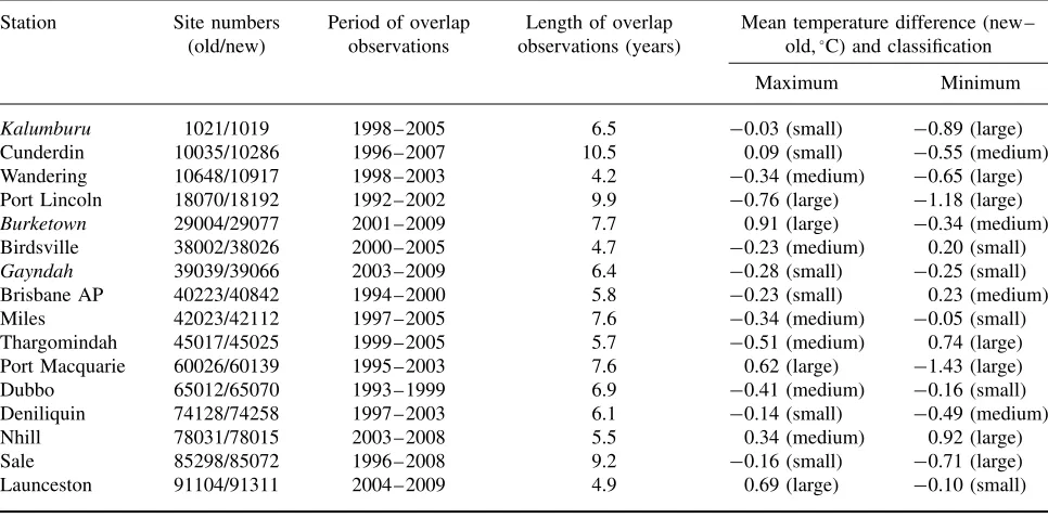
Table I. Site pairs used for adjustment technique evaluation (stations in italics not used for the 1930 network comparisons). Mean temperature differences were classified as large if they exceeded 0.6°C, medium if they exceeded 0.3°C annually or 0.5°C in
any season, and small otherwise.
Station Site numbers (old/new)
Period of overlap observations
Length of overlap observations (years)
Mean temperature difference (new– old,°C) and classification
Maximum Minimum
Kalumburu 1021/1019 1998–2005 6.5 −0.03 (small) −0.89 (large)
Cunderdin 10035/10286 1996–2007 10.5 0.09 (small) −0.55 (medium)
Wandering 10648/10917 1998–2003 4.2 −0.34 (medium) −0.65 (large)
Port Lincoln 18070/18192 1992–2002 9.9 −0.76 (large) −1.18 (large)
Burketown 29004/29077 2001–2009 7.7 0.91 (large) −0.34 (medium)
Birdsville 38002/38026 2000–2005 4.7 −0.23 (medium) 0.20 (small)
Gayndah 39039/39066 2003–2009 6.4 −0.28 (small) −0.25 (small)
Brisbane AP 40223/40842 1994–2000 5.8 −0.23 (small) 0.23 (medium)
Miles 42023/42112 1997–2005 7.6 −0.34 (medium) −0.05 (small)
Thargomindah 45017/45025 1999–2005 5.7 −0.51 (medium) 0.74 (large)
Port Macquarie 60026/60139 1995–2003 7.6 0.62 (large) −1.43 (large)
Dubbo 65012/65070 1993–1999 6.9 −0.41 (medium) −0.16 (small)
Deniliquin 74128/74258 1997–2003 6.1 −0.14 (small) −0.49 (medium)
Nhill 78031/78015 2003–2008 5.5 0.34 (medium) 0.92 (large)
Sale 85298/85072 1996–2008 9.2 −0.16 (small) −0.71 (large)
Table II. Adjustment methods evaluated in this study.
Method Definition
(a) No adjustment (the ‘control’ case)
(b) PM99 algorithm, using the 10 nearest neighbours with available daily data over the evaluation period
(c) As for (b), but considering only neighbours which also had available daily data in 1930 (to test the performance of methods using sparser networks typical of earlier years).
(d) As for (b), but using the PM95 algorithm (e) As for (b), but using the PM90 algorithm
(f) As for (d), but using a maximum of five neighbours
(g) Monthly adjustments, using the 10 nearest neighbours with available monthly data over the evaluation period (h) As for (g), but considering only those neighbours which also had available monthly data in 1930
(i) The QM algorithm used in the RHtestsV3 software (Wanget al., 2010)
A separate evaluation was carried out to assess explic-itly the effect of correlation of reference stations on the effectiveness of the PM95 method. This evaluation used only those stations (eight for maximum temperature, four for minimum) where there were at least 15 potential refer-ence stations with a correlation of 0.8 or better. For each station/element, separate adjustments were made, and the metrics above calculated, for a series of separate trials, using five separate sets of ten reference stations drawn randomly from all those stations correlated with the can-didate station at better than 0.8, 0.7 and 0.6, respectively (15 trials in total). The results from this evaluation are shown in Table V.
The key points to emerge from the evaluation are as follows:
• No adjustment method consistently outperforms the control case for stations with small inhomogenities (Table III), suggesting that 0.3°C is near the lower limit for the size of inhomogeneity that can be adjusted for with useful skill (Figure 8).
• The quantile-matching (QM) method performs more poorly than the PM family for almost all metrics, and only outperforms the control case for maximum temperature for stations with large inhomogeneities, although for minimum temperature it also outperforms the control case for stations with medium inhomo-geneities. It should be noted that the QM method does not use reference series for adjustment (although this is planned in future versions; X. L. Wang, pers. comm.), and is hence likely to perform poorly when applied in situations where there are rapid changes in the back-ground climate; the results for maximum temperature in this evaluation are driven to a large extent by par-ticularly poor results for four stations in inland New South Wales and Queensland, a region where 5 year mean maximum temperatures warmed by up to 1°C over the 1992–2009 period.
• There is little difference between the daily (PM) and monthly adjustment methods for the RMS and proportion within 0.5°C metrics. However, the daily methods outperform the monthly methods substantially in simulating extremes, especially for stations with
large inhomogeneities, except for some extent for extreme high maximum temperatures.
• The PM95 method performs similarly to PM99 on the first three metrics, but is generally much better than PM99 in simulating the highest and lowest values. It is likely that this reflects instability in the transfer functions towards the ends of the distribution when the 1st and 99th percentiles are used; in most cases those percentiles are based on only a few observations, and may therefore be vulnerable to data quality issues at neighbour stations, or effects of unusual weather events. The PM90 method performs marginally worse than PM95 on most measures.
• The five-neighbour case performs marginally worse than the ten-neighbour case on most measures. • Across the set of evaluation stations as a whole, the
rel-ative performance of daily and monthly methods using the 1930 network was similar to that using the more recent network. However, at some individual stations where the availability of neighbouring monthly data in 1930 was much better than that of neighbouring daily data, the monthly adjustment method outperformed daily methods.
Whilst the performance of the PM95 method generally declines with decreasing correlation of reference stations, it still outperforms both monthly adjustments and the control case for stations with medium or large inho-mogeneities for reference station correlations of 0.6 or above. This contrasts with the results of Della-Marta and Wanner (2006) and Mestreet al. (2011) who found that a reference station correlation of greater than 0.8 was required. Whilst a full reconciliation of these different results is beyond the scope of this article, some dif-ferences between this evaluation and those presented in the aforementioned article, which may be relevant to the results, include:
• The earlier methods both use a single reference station rather than a combination of multiple reference sta-tions, and their evaluation is carried out using a single base data set.
Table III. Comparison of adjustment methods, current network (S – small; M – medium; L – large).
Test Variable Station
type
Adjustment method
None Daily PM99
Daily PM95
Daily PM90
Monthly Five neighbours
RHtests
RMS (°C) Maximum All 0.808 0.711 0.704 0.703 0.702 0.705 0.991
S 0.604 0.637 0.642 0.631 0.595 0.557 0.843 M/L 0.930 0.754 0.742 0.746 0.766 0.744 1.080 L 1.263 0.888 0.865 0.879 0.931 0.856 1.077
Minimum All 1.126 0.913 0.908 0.910 0.950 0.911 1.021
S 0.697 0.741 0.731 0.727 0.707 0.720 0.828 M/L 1.321 0.991 0.988 0.993 1.061 0.998 1.108 L 1.451 1.003 1.000 1.006 1.092 1.009 1.099
Prop within 0.5°C Maximum All 0.491 0.568 0.568 0.572 0.588 0.567 0.331
S 0.598 0.590 0.586 0.595 0.627 0.596 0.370 M/L 0.426 0.554 0.557 0.558 0.565 0.549 0.307 L 0.280 0.520 0.528 0.525 0.536 0.531 0.385
Minimum All 0.399 0.467 0.472 0.469 0.449 0.474 0.396
S 0.594 0.552 0.559 0.558 0.573 0.567 0.432 M/L 0.310 0.429 0.433 0.429 0.392 0.431 0.380 L 0.262 0.417 0.423 0.418 0.368 0.423 0.381 Indices count Maximum 10th percentile All 28.7 15.4 14.6 12.8 17.1 13.4 55.2
(mean percent S 14.7 16.7 14.9 13.4 10.9 12.2 39.8
error) M/L 37.1 14.6 14.4 12.5 20.8 14.1 64.5
L 65.1 18.1 15.2 15.7 38.5 15.8 81.1
Minimum 10th percentile All 75.4 17.4 16.0 18.4 28.5 16.3 40.6
S 13.9 8.8 7.5 10.0 8.0 8.8 26.6
M/L 103.4 21.3 19.8 22.3 37.8 19.7 47.0
L 143.4 23.5 20.6 23.9 52.9 20.1 53.3
Maximum 90th percentile All 28.3 11.3 11.8 11.3 11.0 12.1 31.3
S 12.9 14.6 15.2 13.9 8.6 15.2 28.1
M/L 37.5 9.3 9.8 9.8 12.4 10.1 33.2
L 67.3 10.4 12.4 12.2 11.8 12.1 37.2
Minimum 90th percentile All 16.6 11.7 9.9 9.5 19.9 9.8 20.4
S 8.8 9.1 8.7 7.9 14.6 8.9 22.1
M/L 20.2 13.0 10.4 10.2 22.3 10.2 19.6
L 23.2 15.1 11.1 10.2 22.9 10.5 14.9
Extremes error Lowest maximum All 0.46 0.60 0.50 0.49 0.49 0.50 0.71
(°C) S 0.50 0.65 0.59 0.37 0.52 0.41 0.67
M/L 0.44 0.58 0.45 0.55 0.48 0.54 0.74
L 0.55 0.68 0.49 0.56 0.66 0.54 0.71
Lowest minimum All 1.19 0.78 0.69 0.75 0.85 0.70 0.89
S 0.56 0.68 0.55 0.57 0.48 0.54 0.61
M/L 1.48 0.82 0.76 0.84 1.01 0.78 1.02
L 1.64 0.81 0.71 0.83 1.05 0.71 0.94
Highest maximum All 0.76 0.73 0.61 0.63 0.65 0.63 0.90
S 0.59 0.70 0.67 0.57 0.58 0.53 0.78
M/L 0.87 0.75 0.58 0.65 0.69 0.68 0.98
L 1.22 1.01 0.70 0.63 0.94 0.66 0.85
Highest minimum All 0.54 0.66 0.58 0.59 0.69 0.60 0.69
S 0.47 0.60 0.58 0.58 0.56 0.57 0.70
M/L 0.58 0.69 0.58 0.59 0.74 0.61 0.69
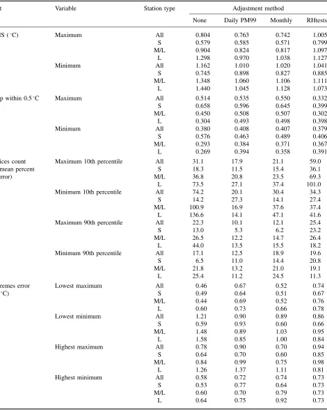
Table IV. Comparison of adjustment methods, 1930 network.
Test Variable Station type Adjustment method
None Daily PM99 Monthly RHtests
RMS (°C) Maximum All 0.804 0.763 0.742 1.005
S 0.579 0.585 0.571 0.799
M/L 0.904 0.824 0.817 1.097
L 1.298 0.970 1.038 1.127
Minimum All 1.162 1.010 1.020 1.041
S 0.745 0.898 0.827 0.885
M/L 1.348 1.060 1.106 1.111
L 1.440 1.045 1.128 1.073
Prop within 0.5°C Maximum All 0.514 0.535 0.550 0.332
S 0.658 0.596 0.645 0.399
M/L 0.450 0.508 0.507 0.302
L 0.304 0.493 0.498 0.398
Minimum All 0.380 0.408 0.407 0.379
S 0.576 0.463 0.489 0.406
M/L 0.293 0.384 0.371 0.367
L 0.269 0.394 0.358 0.391
Indices count Maximum 10th percentile All 31.1 17.9 21.1 59.0
(mean percent S 18.3 11.5 15.4 36.1
error) M/L 36.8 20.8 23.5 69.3
L 73.5 27.1 37.4 101.0
Minimum 10th percentile All 74.2 20.1 30.4 34.3
S 14.2 27.3 14.1 27.4
M/L 100.9 16.9 37.6 37.4
L 136.6 14.1 47.1 41.6
Maximum 90th percentile All 22.3 10.1 12.1 25.4
S 13.0 5.3 6.2 23.2
M/L 26.5 12.2 14.7 26.4
L 44.0 13.5 15.5 18.2
Minimum 90th percentile All 17.1 12.5 18.9 19.6
S 6.5 11.0 14.4 20.8
M/L 21.8 13.2 21.0 19.1
L 25.4 11.2 24.5 11.3
Extremes error Lowest maximum All 0.46 0.67 0.52 0.74
(°C) S 0.49 0.64 0.51 0.67
M/L 0.44 0.69 0.52 0.76
L 0.60 0.73 0.66 0.78
Lowest minimum All 1.21 0.90 0.89 0.86
S 0.59 0.93 0.60 0.66
M/L 1.48 0.89 1.03 0.95
L 1.58 0.85 1.00 0.84
Highest maximum All 0.78 0.90 0.70 0.94
S 0.64 0.70 0.60 0.85
M/L 0.84 0.99 0.75 0.98
L 1.26 1.37 1.11 0.81
Highest minimum All 0.58 0.72 0.74 0.73
S 0.53 0.77 0.64 0.73
M/L 0.60 0.70 0.79 0.73
0 0.2 0.4 0.6 0.8 1 1.2 1.4 1.6
Maximum -all
Maximum -med/large
Maximum -large
Minimum -all
Minimum -med/large
Minimum -large
None PM95 Monthly RHtestsV3
0 20 40 60 80 100 120 140 160
Maximum -all
Maximum -med/large
Maximum -large
Minimum -all
Minimum -med/large
Minimum -large
None PM95 Monthly RHtestsV3
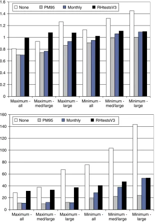
Figure 7. Performance measures of adjustment techniques across different classifications of station pairs: (top) RMS error (°C), (bottom) percent error in count of days with maximum above 90th percentile and minimum below 10th percentile. This figure is available in colour online at
wileyonlinelibrary.com/journal/joc
• Both earlier methods carry out their evaluation using a synthetic data set where the correlation is degraded using a random noise process, and an idealized set of inhomogeneities. In practice, it is likely that some of the degradation of correlation between neighbouring stations below 1.0 is due to factors such as time shift-ing (through the movement of synoptic-scale weather systems) or non-linearity of the relationship between temperatures at the two stations, and is not truly random. Furthermore, the behaviour of the inhomo-geneities at the range of stations used for evaluations in this article may not match the idealized examples used in earlier studies.
• The evaluation in this article uses a wider range of metrics than Della-Marta and Wanner (2006) (although a similar range to that of Mestre et al., 2011). In general, the improvement which the PM methods offer
-0.4 -0.2 0 0.2 0.4 0.6 0.8 1
0 0.2 0.4 0.6 0.8 1 1.2 1.4 1.6
Mean inter-site temperature difference (deg C)
RMS difference (deg C)
Figure 8. Difference in RMS errors (no adjustment – PM95 algorithm) for station pairs, by size of mean temperature differences between
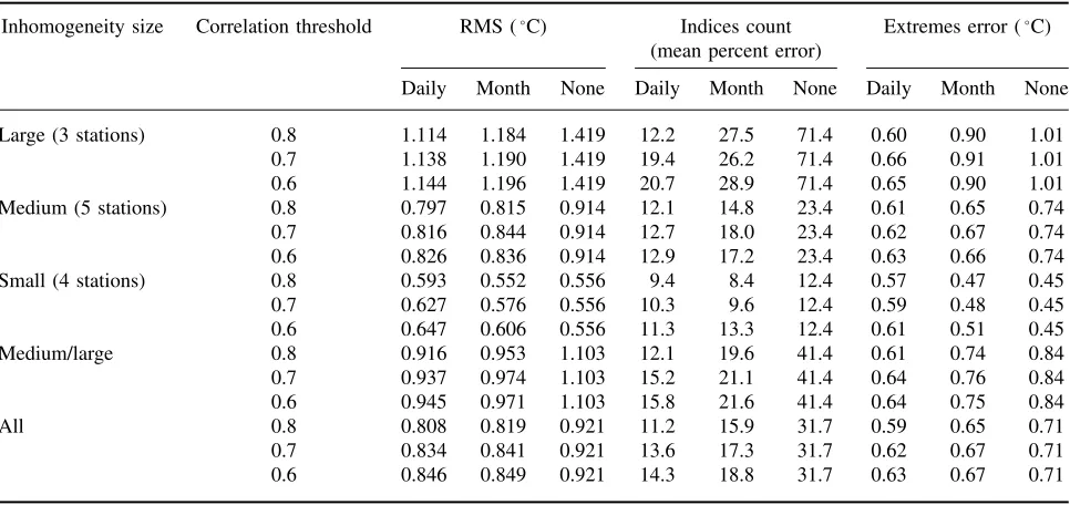
Table V. Evaluation of adjustment methods for different reference series correlation thresholds.
Inhomogeneity size Correlation threshold RMS (°C) Indices count (mean percent error)
Extremes error (°C)
Daily Month None Daily Month None Daily Month None
Large (3 stations) 0.8 1.114 1.184 1.419 12.2 27.5 71.4 0.60 0.90 1.01
0.7 1.138 1.190 1.419 19.4 26.2 71.4 0.66 0.91 1.01
0.6 1.144 1.196 1.419 20.7 28.9 71.4 0.65 0.90 1.01
Medium (5 stations) 0.8 0.797 0.815 0.914 12.1 14.8 23.4 0.61 0.65 0.74
0.7 0.816 0.844 0.914 12.7 18.0 23.4 0.62 0.67 0.74
0.6 0.826 0.836 0.914 12.9 17.2 23.4 0.63 0.66 0.74
Small (4 stations) 0.8 0.593 0.552 0.556 9.4 8.4 12.4 0.57 0.47 0.45
0.7 0.627 0.576 0.556 10.3 9.6 12.4 0.59 0.48 0.45
0.6 0.647 0.606 0.556 11.3 13.3 12.4 0.61 0.51 0.45
Medium/large 0.8 0.916 0.953 1.103 12.1 19.6 41.4 0.61 0.74 0.84
0.7 0.937 0.974 1.103 15.2 21.1 41.4 0.64 0.76 0.84
0.6 0.945 0.971 1.103 15.8 21.6 41.4 0.64 0.75 0.84
All 0.8 0.808 0.819 0.921 11.2 15.9 31.7 0.59 0.65 0.71
0.7 0.834 0.841 0.921 13.6 17.3 31.7 0.62 0.67 0.71
0.6 0.846 0.849 0.921 14.3 18.8 31.7 0.63 0.67 0.71
over monthly adjustments is more evident in extremes-based metrics than it is in the RMS error.
9. Implementation of adjustment methods for the ACORN-SAT network
Following the evaluation of the PM algorithm and other methods, adjustment methods were implemented for the ACORN-SAT network using the following rules:
• Other than in the specific cases outlined below, the PM95 method was used. Neighbours (up to ten) were selected in descending order of correlation with the candidate station, with a lower correlation limit of 0.6. (For the purpose of this section, the ‘correlation’ value was derived by taking correlations between daily temperature anomalies for each of the 12 months, with the final value taken as the 6th highest – i.e. near the median – of these 12 values.)
• If fewer than three sufficiently correlated stations existed with daily data around the time of the inho-mogeneity, or the tenth best-correlated station with monthly data was better correlated than the third best-correlated station with daily data, the monthly adjust-ment method was used. In a few cases neighbours with correlations between 0.5 and 0.6 were used to provide at least three reference stations. (Had there been any location with no available reference series, the RHt-estsV3 method, which does not use reference series, would have been an option.)
• In the event of a ‘spike’ (defined as an inhomogeneity, followed by another inhomogeneity of opposite sign within 3 years, or alternatively two metadata-defined inhomogeneities within 3 years), monthly adjustments were used to adjust the data during the ‘spike’ period to the period before the ‘spike’, as daily adjustments
were considered to be too unstable for such short-period corrections. These were only implemented if the annual mean adjustment during the ‘spike’ period was at least 0.5°C. The ‘spike’ period was also excluded from the overlaps used for the calculation of transfer functions for other inhomogeneities.
• The size of adjustments generated by the techniques above was checked by comparing the means of pre-and post-adjustment data for, in general, the five cal-endar years prior to the inhomogeneity. The adjustment was only implemented if the means differed by at least 0.3°C on an annual basis, 0.3°C (not necessarily of the same sign) in at least two of the four seasons, or 0.5°C in at least one season. If the difference failed to satisfy one or more of these criteria the inhomogeneity was considered to be too small to justify adjustment, as the results of the evaluation above suggest that such small adjustments add no skill.
• A special case was the 1965 move at Albany in southern Western Australia from the town to the airport, with no overlap. A station was re-established in Albany town in 2002 and monthly data indicated it was approximately homogeneous with the pre-1965 town station (and much better correlated with the airport than any other neighbour was). The post-2002 town site was therefore used as a proxy for the pre-1965 site, with the adjustments for the 1965 move calculated using a transfer function derived from the 2004 to 2009 overlap.
pairwise comparison of ACORN-SAT time series was undertaken, and the robustness of adjustments checked by recalculating them using subsamples of neighbour sta-tions. As a result of this process, a number of adjustments were recomputed using different sets of neighbour sta-tions (most often because one or more neighbours were inhomogeneous), or with time periods other than those immediately preceding/following the inhomogeneity used to derive transfer functions (most often because a station deterioriated sharply in the 1–2 years prior to a move or other change).
In a small number of cases, the PM95 algorithm was not able to homogenize extreme values, as the rela-tionship between sites for 95th (or 5th) percentile val-ues is not representative of that for the most extreme values. This mostly occurs with extreme high maxima at near-coastal locations (Figure 1), where large differences between sites on 95th percentile days collapse to near zero on the very hottest days when offshore winds over-ride the sea breeze. Stations which showed evidence of one or more inhomogeneities of 2°C or more in the time series (highest value of year – 95th percentile value for year), or equivalently for low extremes, were considered unhomogenizable for extremes and excluded from some downstream products. Four stations, all coastal, failed this test: Albany and Port Macquarie for high maximum temperatures, Eucla for high minimum temperatures and Horn Island for low minimum temperatures.
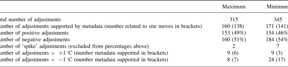
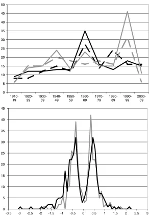
The total number of adjustments, the frequency distri-bution of adjustments, and the distridistri-bution of positive and negative adjustments through time, are given in Table VI and Figure 9. Positive and negative adjustments are fairly evenly balanced for maximum temperatures, but negative adjustments (i.e. where there has been an artificial drop in temperatures as a result of an inhomogeneity) are some-what more numerous for minimum temperature, which is likely to result in the ACORN-SAT minimum tem-perature showing a stronger warming trend than the raw data do.
The imbalance between positive and negative adjust-ments for minimum temperature is concentrated in the 1940s and 1990s, which coincides with the two main periods in which stations moved from town centres to out-of-town locations (mostly airports) a move which typ-ically results in a drop in minimum temperatures. Most of the positive adjustments in minimum temperature in
the 1960s are small adjustments associated with changes in observation times in 1964 (see later section).
10. Changes affecting large parts
of the temperature network simultaneously
Changes which affect large parts of the network simulta-neously provide a particular challenge for homogeniza-tion, since they can affect reference series as well as a candidate station, causing assumptions of a locally homogeneous reference series around the time under examination to break down. Furthermore, whilst an inho-mogeneity considered too small for adjustment (less than 0.3°C) under the criteria discussed in the previous sec-tion is unlikely to have a substantial impact on large-scale analyses, such an inhomogeneity occurring across a large part of the network simultaneously could have an impact on indicators such as trends at the national or regional scale.
Three such changes have been identified in the period covered by the ACORN-SAT data set:
• Changes in observation time, principally the shift to an 0900–0900 observation day for maximum and minimum temperature in 1964, as well as the use of 0000/1200 UTC observation day at some AWSs in the 1990s and early 2000s, and the effective shift of observation time by 1 h with the introduction of daylight saving time in some states from the early 1970s onwards.
• The change from imperial to metric measurements which took place on 1 September 1972, and associated changes in the frequency of rounding.
• The introduction of AWSs across large parts of the network from the early 1990s onwards.
10.1. Effect of observation time changes
To estimate the effect of observation time changes which have occurred over time, available 1 min data (mostly from the period 2003–2009) from 32 ACORN-SAT stations were used to calculate daily maximum and minimum temperatures for a range of time periods which have been used historically, as shown in Table VII. These were compared with temperatures measured using the current standard of 0900–0900 local time. This study, and its results, is described in more detail in Trewin (2012).
Table VI. Summary of adjustments carried out in ACORN-SAT data set.
Maximum Minimum
Total number of adjustments 315 345
Number of adjustments supported by metadata (number related to site moves in brackets) 160 (138) 171 (141)
Number of positive adjustments 153 (49%) 154 (46%)
Number of negative adjustments 160 (51%) 184 (54%)
Number of ‘spike’ adjustments (excluded from percentages above) 2 7
0 5 10 15 20 25 30 35 40 45 50
1910-19
1920-29
1930-39
1940-49
1950-59
1960-69
1970-79
1980-89
1990-99
2000-09
0 5 10 15 20 25 30 35 40 45
-3.5 -3 -2.5 -2 -1.5 -1 -0.5 0 0.5 1 1.5 2 2.5 3
Figure 9. (top) Number of positive (black) and negative (grey) adjustments by decade, for maximum (dashed line) and minimum (solid line) temperature (bottom). Frequency distribution of mean annual adjustment size (°C) for maximum (grey) and minimum (black) temperature.
The 1 min data indicate that the only historical obser-vation practice which shows substantial systematic dif-ferences from the current standard is the measurement of minimum temperatures using 0000–0000 day (i.e. mid-night to midmid-night). Averaged across the 32 stations, this gives mean minimum temperatures 0.25°C cooler than the current standard, whilst the impact on extremes is stronger, with the mean value of the highest minimum temperature of each month being 0.58°C cooler on aver-age. All 32 stations show cooler minimum temperatures for 0000–0000 day than 0900–0900 day, but the differ-ences were smallest (typically near 0.1°C) in the trop-ics. They were largest (0.4–0.6°C) at some southern coastal stations. As about 30% of the network was using 0000–0000 day in some form prior to 1964, these results would suggest a potential inhomogeneity in Australian mean minimum temperatures of approximately+0.08°C in 1964.
As a result of these findings, it was decided to define 1 January 1964 as a metadata indicated potential
inhomogeneity at all locations which were believed to use 0000–0000 day prior to 1964, were outside the tropics and had not already had an adjustment made in the 1962–1966 period, and to adjust for that inhomogeneity, excluding stations subject to 0000–0000 day as reference series, whether or not it reached the 0.3°C threshold defined as a minimum for adjustment in earlier sections (this takes into account the likelihood of extremes being affected more significantly than means).
Table VII. Comparison of major observation times in previous use with current standard.
Method In use Temperature differences with current
(0900–0900 local clock time) standard (°C) Mean
maximum
Mean minimum
Highest monthly minimum
Lowest monthly maximum
Maximum and minimum 0000–0000 (standard time)
1932–1963 at Bureau-staffed sites (and a few others)
−0.01 −0.25 −0.58 0.00
Maximum and minimum 0900–0900 standard time (i.e. no daylight saving)
1964–1972, later in states without daylight saving
0.00 −0.01 −0.05 −0.01
Maximum 1200–1200 UTC, minimum 0000–0000 UTC
Some AWSs from early 1990s to mid-2000s
0.02 −0.01 (−0.06 WA, 0.06 NSW/Vic/Tas)
−0.04 (−0.23 WA, 0.24 NSW/Vic/Tas)
0.08
Maximum 0900–0900 standard time (reverting to 0900–1500 if 0900 reset temperature within 0.5°C of
maximum), minimum 1500–0900 standard time
Non-Bureau-staffed sites pre-1964
−0.03 0.03 0.13 −0.12
resultant inhomogeneity had already been detected and adjusted for as part of the main ACORN-SAT procedures.
10.2. Effect of metrication
Metric measurements for temperature were introduced across the Australian network on 1 September 1972, with new instruments being issued to all stations. Pre-vious research (Nicholls, 2004) had found no discernable impact of this change on temperatures. These conclu-sions, however, were partly based on the results of instru-ment testing for which no docuinstru-mentation could be located at the time of the current project. It was therefore decided to carry out a number of further tests, these being:
• Comparison of Australian mean temperatures with sea surface temperatures in the Australian region.
• Comparison of mean temperatures at ACORN-SAT locations where upper-air observations were taken with the mean 850 hPa temperatures at those locations. • Comparison of mean maximum and minimum
peratures at ACORN-SAT locations with the tem-peratures at 1500 and 0600, respectively (excluding locations/months where daylight saving time was in use).
Whilst the comparison data sets are not independent in the sense that they also changed to metric measurements at or near the same time, they used different instruments and hence an inhomogeneity affecting a particular instrument type could be detected by these methods.
All three comparisons showed mean Australian tem-peratures in the 1973–1977 period were from 0.07 to 0.13°C warmer, relative to the reference series used, than those in 1967–1971. However, interpretation of these results is complicated by the fact that the temperature relationships involved (especially those between land and
sea surface temperatures) are influenced by the El Ni˜no-Southern Oscillation (ENSO), and the 1973–1977 period was one of highly anomalous ENSO behaviour, with major La Ni˜na events in 1973–1974 and 1975–1976. It was also the wettest 5 year period on record for Aus-tralia, and 1973–1975 were the three cloudiest years on record for Australia between 1957 and 2008 (Jovanovic
et al., 2011).
The broad conclusion is that a breakpoint in the order of 0.1°C in Australian mean temperatures appears to exist in 1972, but that it cannot be determined with any certainty the extent to which this is attributable to metrication, as opposed to broader anomalies in the climate system in the years following the change. As a result, no adjustment was carried out for this change.
10.3. Introduction of AWSs
AWSs were introduced widely across the network from the early 1990s onwards. In many cases, their introduc-tion coincided with a staintroduc-tion move (often with a period of parallel observations). In other cases, they were intro-duced without any site move.