JHS, Vol. 3, Issue 2

(1)

(2)

AUTUMN 2017, Vol 3, No II, JOURNAL OF HYDRAULIC STRUCTURES

Journal of Hydraulic Structures

Department of Civil Engineering

Shahid Chamran University of Ahvaz

In the name

of GOD

(3)

HYDRAULIC

STRUCTURES

SHAHID CHAMRAN UNIVERSITY OF AHVAZ

Manager: Prof. Hamid R. Ghafouri Editor-in-chief: Dr. Ali Haghighi

Editorial coordinator:Dr. Seyed Mohammad Ashrafi Department of Civil Engineering, Engineering Faculty, Shahid Chamran University of Ahvaz, Ahvaz, Iran.

Members

Prof. Hossein M. V.Samani

Civil Engineering Department, Shahid Chamran University of Ahvaz, Ahvaz, Iran

Prof. Hamid R. Ghafouri

Dr. Ali Haghighi

Prof. Mahmood S. Bajestan

Hydraulic Structures Department, Shahid Chamran University of Ahvaz, Ahvaz, Iran

Prof. Saeed R. S. Yazdi

Civil Engineering Department, K.N.Toosi University of Technology, Tehran, Iran

Dr. Mohammad S. Pakbaz

Dr. Arash Adib

Civil Engeering Department, Shahid Chamran University of Ahvaz, Ahvaz, Iran

Dr. Mojtaba Labibzadeh

Prof. Helena M. Ramos

Instituto Superior Técnico (IST), University of Lisbon Dr. S. Mohammad Ashrafi

Dr. S. Abbas Haghshenas

Institute of Geophysics, University of Tehran | UT, Tehran, Iran Dr. Mohammad Zounemat-Kermani

Department of Water Engineering, Shahid Bahonar University of Kerman, Kerman, Iran

Dr. Taher Rajaee

Civil Engineering Department, University of Qom, Qom, Iran Dr. Mohammad Vaghefi

Civil Engineering Department, Faculty of Engineering, Persian Gulf University, Bushehr, Iran

Dr. A. A. Telvari

Soil Conservation and Watershed Management Research Institute; Department of Civil Engineering, Islamic Azad University, Ahvaz branch, Ahvaz, Iran

II

Aims and Scope

01 Investigating the vulnerability downstream

area of Taleghan dam due to dam failure

H. Goharnejad; M. Azizkhani; M. Zakeri Niri; S. Moazami

10 An experimental study on hydraulic

behavior of free-surface radial flow in

coarse-grained porous media

A. Rajabi; E. Hatamkhani; J. Sadeghian

22 Three-dimensional numerical modeling of

score hole in rectangular side weir with

finite volume method

S. Ghotbi; A. Abdollahi; M. Azhdari Moghadam

32 Experimental Study of the Effect of

Base-level fall at the Beginning of the Bend on

Reduction of Scour around a Rectangular

Bridge Pier Located in the 180 Degree

Sharp Bend

M. vaghefi; M. moghanloo; D. Dehghan; A. keshavarz

47 Developing optimal operating reservoir

rule-curves in drought periods

S. Alahdin; H.R. Ghafouri

62 Finding the Causes and Evaluating Their

Impacts on Urmia Lake Crisis

‎

Using a

Comprehensive Water Resources

Simulation Model

(4)

Aims and Scope

Hydraulic Structure Journal is an interdisciplinary journal which publishes high-quality peer-reviewed articles addressing the latest developments and applied methods in construction, maintenance, management, and operation policy of Hydraulic Structures.

The Journal aims at providing an efficient route to fast-track publication, within 10-12 weeks after manuscript submission. Manuscripts will be considered for publication in the following categories: research articles, technical notes, case reports and discussions.

The general areas covered by the Journal include:

 Technical and methodological advances in application, design/selection, production, modification of construction materials

 Advances in numerical and analytical methods  Hydro informatics and soft computing  Hydraulic aspects of hydraulic structures

 Applied surface and subsurface hydrology and hydrometeorology  Forecasting approaches in water resources engineering

 Economic and social aspects of hydraulic structures

 Uncertainty analysis and risk management in hydraulics and water resources engineering  Application of Nanotechnology in Hydraulic Structures

 Geotechnics of Hydraulic Structures  Damage detection techniques

The following might be considered as hydraulic structures:

 Dams and associated structures  River and Watershed Structures  Offshore and Onshore Structures

 Irrigation and Drainage Channel Networks  Bridges

 Water Storage and Conveyance Structures  Pipelines and Pump Stations

 Sewerage Systems

 Water and Wastewater Treatment Plants  Historical Water Structures

General Information

Title: Journal of Hydraulic Structures

Subject: Hydraulics and water resources engineering Coverage area: International

Journal Type: Scientific and technical License Holder: Shahid Chamran University Editor-in-Chief: Dr. Ali Haghighi

Manager: Prof. Hamid R. Ghafouri

Editorial coordinator: Dr. Seyed Mohammad Ashrafi

Language Editors: Majid SadollahKhani Soroosh Kamali

Address: Engineering Faculty, Shahid Chamran University of Ahvaz

Phone #: +986113330010-20 (5610 & 5603)

(5)

AUTUMN 2017, Vol 3, No 2, JOURNAL OF HYDRAULIC STRUCTURES Shahid Chamran University of Ahvaz

Journal of Hydraulic Structures

J. Hydraul. Struct., 2017; 3(2):1-9 DOI: 10.22055/jhs.2017.13435

Investigating the vulnerability downstream area of Taleghan

dam due to dam failure

Hamid Goharnejad1 Mahyar Azizkhani2 Mahmoud Zakeri Niri3 Saber Moazami4

Abstract

Due to the immense damage caused by dam failure, especially dams constructed near large cities, it is necessary to consider the breaking phenomena as well as studying and designing different parts of the dam. For this purpose, the hydrograph of the outflow due to dam failure must be identified according to size of the fracture and then flood routing, and flood zone must be determined based on the downstream topography and morphology. The integration of hydraulic models and geographic information system is used to achieve this objective. In this research the effect of breaking Taleghan storage dam due to the slip of a pile of reservoir abutment and the creation of current wave toward the dam body as well as the vulnerability analysis due to the breaking of the dam on downstream lands was studied. At first, Taleghan dam failure for five different scenarios was modeled using the FLOW-3D numerical software and then the geometric data of the river was extracted using the ArcGIS software and modeling the flood due to dam failure was conducted in Hec-GeoRas model. Then, the risk analysis was performed for each break scenario of Taleghan dam. The results indicated that the maximum amount of inundation would occur in Razmian city at an approximate distance of 45 kilometers from Taleghan dam site.

Keywords: Dam breaking, Inundation, Vulnerability, Risk analysis, Taleghan dam.

Received: 17 September 2017; Accepted: 07 November 2017

1_{Department of Civil Engineering, Environmental Sciences Research Center, Islamshahr Branch, Islamic}

Azad university, Islamshahr, Iran, [email protected] (Corresponding author)

Azad university, Islamshahr, Iran, [email protected].

Azad university, Islamshahr, Iran, [email protected]

4 _{Department of Civil Engineering, Environmental Sciences Research Center, Islamshahr Branch, Islamic}

(6)

1. Introduction

Dams are always considered as a potential threat for their downstream areas because of creation of large water reservoirs. Dam designers attempt to lower vulnerability potentials by applying safety factors; however, natural and non-natural factors like floods, piping phenomenon, foundation weakness and exploding can cause a dam to break [1]. The problem of dam failure and effects of surges on downstream areas attracted many scholars and experts' attention, after several important dams like Teton were broken [2]. To reduce the effects of a large reservoir dam failure, it is important to know the changes of hydraulic parameters due to break in dam, such as depth, speed, flow, and the time when the wave forehead reaches the downstream area and finally to determine the border and designing the flood zone in order to reduce the financial losses and casualties. In this regard, in the last few decades, different researchers have done numerous theoretical and practical studies in order to determine the mechanism of dam failure and the trends of hydraulic parameters as a function of time and space [3]. One of the most important methods for erosion control in rivers in these situations is ston masonery and riprap. A general dimensionless equation for the prediction of maximum particle size of stable riprap into the tributary channel at river confluences has been developed by Ghanbari Adivi et al. [4]. Their results showed that the stability number of riprap into the tributary channel increases with increasing the ratio of tailwater depth to particle size.

Fliervoet et al. [5], Lim [6] and Chiew [7] found that during flooding, the emergence of various forms such as Ripple and Dune and live bed is natural. These processes, despite the intersectional structures, can cause inconstancy in these structures. Andam [8] investigated the changes in speed and number of landing by using HECGeo-RAS model in a research entitled as the comparison of river regime inside and outside of forest area, and compared the influence of vegetation on the physical behavior of the flow. He concluded that using the HECGeo-RAS model can offer researchers suitable numbers to study the diet and other hydraulic characteristics of river flow. Sholtes [10] used HEC-RAS software to route flood dynamics in rural and urban areas of Northern California and concluded that the decrease in slope and increase in roughness of floodplain and river have more influence on flood attenuation. Nagy et al., [11] investigated the sand grinding attrition and meanders evolution in an answer to Tisza River engineering in Hungary and found that due to severe attrition in the area and human intervention (performing engineering projects), this river has reached a balance by shortcuts in its route. However, the purpose of this article is to investigate and determine the flood plain area. Then the amount of vulnerability risk over all path of the river for five different scenarios of dam break and for wave arrival times of 30 and 120 minutes were identified.

2. Methodology

The conducted research is presented in details in this section.

2.1. Study area

(7)

Figure 1. Map of Taleghan river in Taleghan dam downstream

2.2 Physical characteristics of Taleghan river in Taleghan dam downstream

In order to perform the model, it is necessary to determine the river characteristics such as the left and right bank, riverbed, and roughness coefficient of each section. Therefore, after several field studies and inspections, the required data were determined and entered the model. Then using the Arc-GIS, the cross sections were provided and entered the model. Considering the high length of the study area, the distance of cross sections in straight parts of the river was chosen about 4000 meters and 1500 meters in sudden intersections and arches. Among the factors affecting the manning coefficient are the grading substrate material, the rippling degree of river, the relative effect of obstacles, the density of vegetation and morphology form of the river. Therefore, in order to determine and estimate the manning coefficient in a part of river, it should be divided to three main parts including the mainstream and flood plains of right and left banks. Because of the important role of roughness coefficient, the model were calibrated using this parameter.

2.3 Determining boundary conditions

(8)

suitable level of water in upstream.

2.4 Discharge inflow

Five scenarios are defined to investigate embankment dam failure resulting from overtopping. Inflow volume to the reservoir is different in each scenario. Based on the reviews, minimum flood volume that overtops and damages the dam body is about 5 MCM. In addition, maximum flood volume that fully destroys the dam body is about 25 MCM. In the range of 5 to 25 MCM, flood volumes of 7.5, 9 and 13 MCM have been considered. The charecteristics of scenarios have been presented in Table 1. ([12])

Table1. Flow modeling conditions for five states of overtopping in Taleghan dam

Scenario Water Height in Reservoir (m)

Storage (MCM)

Flood Volume (m3)

Flood Discharge (cms)

1 82 420 5.0 54,269

2 82 420 7.5 59,390

3 82 420 9.0 78,913

4 82 420 13.0 89,129

5 82 420 25.0 97,054

2.5 The risk taking theory due to dam failure

The researchers consider the three parameters of escape time, velocity, and depth of flooding as the appropriate criteria of dam failure risk. Considering the importance of the escape time in reducing life loss of downstream areas, the 30 to 120 minutes after the beginning of dam failure are selected as the risk criteria of these areas over time [13].

The flow velocity and depth of flooding is considered simultaneously in assessing the consequences of dam failure. In this regard, the flooding area along the river and flood plains and risk index HR are assigned to the grid cells according to the following definition [14].

HR=D(V+0.5) (1)

Table 2. Flood risk levels based on risk amount and risk description [14](Vrouwenvelder et al., 2003.(

HR Flood risk

level Sign Risk description

<0.75 Low R1 Warning: flooded area with shallow running water with deep water remain

0.75 –

1.25 Average R2

Dangerous for some people (For example children): flooded area with deep or fast flowing running water

1.25 – 2.5 High R3 Dangerous for most people: flooded area with deep and fast flowing water

>2.5 Very high R4 Dangerous for everyone: flooded area with deep and fast flowing water

(9)

velocity in meters per second. In general, risk areas are classified into four levels of low, medium, high and very high-risk areas that flood risk levels based on the amount of risk and the descriptions of each level are provided in table 2.

3. Results

Using the HEC-RAS model and geographic information system GIS, modeling the flow of Taleghan river in the downstream of Taleghan dam and caused by the dam break was investigated. Using the topographic data of Taleghan river basin in the downstream of the dam, TIN layer and raster maps of the mentioned area were obtained. Then, using the Hec-GeoRas in the GIS environment, various layers of the river route, banks and river cross sections were prepared. It should be noted that the above data are among the requirements of flow modeling due to dam failure in the HEC-RAS model. After preparing the geometric model of the river, the necessary information was inserted into the HEC-RAS model and flow modeling was carried out after editing the information and peocessing the data.

Modeling the flow for discharges of 54269, 59390, 78913, 89129 and 97054 cubic meters per seconds was conducted. Considering the importance of model calibration after the model simulation, the results for the maximum discharge (scenario 5) and minimum discharge (scenario 1) were calibrated in accordance with the roughness coefficient values. So that the minimum, medium and maximum roughness coefficient values for the right and left side of the river were considered to be respectively as 0.035, 0.040, and 0.045. The minimum, medium, and maximum roughness coefficient values for the riverbed were respectively considered as 0.030, 0.035, and 0.040.

Figure 2. The inundation area due to flooding scenarios 1 to 5 along Taleghan River because of dam breaking

The results indicated that in all studied sections, the amount of water level difference for maximum and minimum roughness coefficients was less than 5%. Therefore, the roughness coefficient values with sufficient accuracy was considered as equal to the average roughness coefficient, that is over the two sides of the river as equal to 0.040 and the river bed as 0.035.

After modeling the flow in HEC-RAS, the data of the flow was exported into the Arc-GIS 4600

4800 5000 5200 5400 5600 5800 6000

54,269 59,390 78,913 89,129 97,054

In

u

n

d

a

tio

n

Ar

ea

(H

ec

)

(10)

and the inundation area for each scenario is provided in Figure 2.

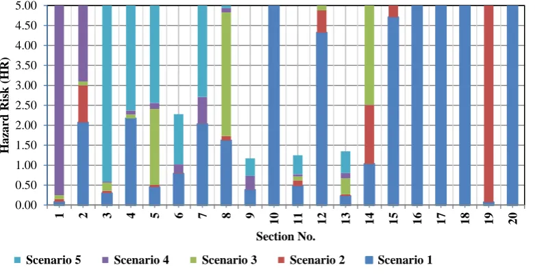
Then, the values of HR index for the escape times of 30 and 120 minutes after the dam break was calculated and provided in figures 3 and 4. For the escape time of 120 minutes and 30 minutes, the sections with high flood risk level (HR> 2.5) are respectively provided in tables 3 and 4.

Figure 3. Risk index values for the escape time of 120 minutes in all sections of the river and different dam failure scenarios

Table 3. Sections with very high-risk levels for the escape time of 120 minutes and different dam failure scenarios

Dam failure scenario

Sections with very high risk levels (HR>2.5)

1 2 3 4 5 6 7 8 9 10 11 12 13 14 15 16 17 18 19 20

1 × × ×

2 × × × × × × × ×

3 × × × × × × × × ×

4 × × × × × × × × × × × ×

5 × × × × × × × × × × × × × × 0.00

0.50 1.00 1.50 2.00 2.50 3.00 3.50 4.00 4.50 5.00

1 2 3 4 5 6 7 8 9

10 11 12 13 14 15 16 17 18 19 20

H

a

za

rd

Risk

(H

R)

Section No.

(11)

Figure 4. Risk index values for the escape time of 30 minutes in all sections of the river and different dam failure scenarios

Table 4. Sections with very high-risk levels for the escape time of 30 minutes and different dam failure scenarios

Dam failure scenario

Sections with very high risk levels (HR>2.5)

1 2 3 4 5 6 7 8 9 10 11 12 13 14 15 16 17 18 19 20

1 × × × × × × ×

2 × × × × × × × × × ×

3 × × × × × × × × × × ×

4 × × × × × × × × × × × × × ×

5 × × × × × × × × × × × × × × × ×

4. Conclusion

Flood plains and areas adjacent to rivers are suitable regions to carry out economic and social activities due to specific conditions. The effect of break and the risk of flooding due to Taleghan dam failure in the downstream area of the dam were investigated in the present study.

Flood zoning due to Taleghan dam failure with discharges of 54269, 59390, 78913, 89129, 97054 cubic meters per second on Taleghan river and the downstream of the dam were investigated. For modeling the study river, HEC-GeoRAS hydraulic model was applied. In the downstream of Taleghan dam, a total of 80 km of the river from the dam site located in the Alborz mountain was modeled. After zoning the areas with a high risk, the vulnerabilities were

0.00 0.50 1.00 1.50 2.00 2.50 3.00 3.50 4.00 4.50 5.00

1 2 3 4 5 6 7 8 9

10 11 12 13 14 15 16 17 18 19 20

H

a

za

rd

Risk

(H

R)

Section No.

(12)

identified. Through calculating the risk index (HR) in any sections of Taleghan river after dam failure, the risk of the flood caused by dam failure in the downstream area was quantified. Therefore, we can easily classify high-risk areas. Observed zoning maps indicate that a great flooding can occur in Razmian city at an approximate distance of 45 kilometers from Taleghan dam site and due to dam failure and also indicate the necessity of adopting special measures to deal with this risk.

References

1. Miller S.N. Kepner W.G. and Mehaffey M.H.2002 .Integration Landscape Assessment and Hydrologic Modeling for Land Cover Change Analysis. Journal of the American Water Resources Association. 38(4):919-929.

4. Ghanbari Adivi, E., Shafai Bajestan, M., Kermannezhad, J., " Riprap sizing for scour protection at river confluence", Journal of Hydraulic Structures J. Hydraul. Struct., 2016; 2(1): 1-11,DOI: 10.22055/jhs.2016.12646

3. Goharnejad, H., Noury, M., Noorzad, A., Shamsaie, A., Gohanejad, A., "The Effect of Clay Blanket Thickness to Prevent Seepage in Dam Reservoir", International Journal of Environmental Sciences, 2010, 4 (6), 556-565.

5. Jan M. Fliervoet, Riyan J.G. van den Born & Sander V. Meijerink (2017) A stakeholder’s evaluation of collaborative processes for maintaining multi-functional floodplains: a Dutch case study, International Journal of River Basin Management, 15:2, 175-186, DOI:10.1080/15715124.2017.1295384

2. Litrico, X. Fromion, V. Baume, J.P. Arranja, C. Rijo, M. 2005. Experimental Validation Of A Methodology To Control Irrigation Canals Based On Saint-Venant Equations. Control Engineering Practice 13 (1425–1437).

7. Chiew, Y. M. 1999. Time scale for local scour at bridge piers. Journal of Hydraulic Engineering, ASCE ,125(1) :59-65.

6. Lim, S. Y., 2001. Parametric study of riprap failure around bridge piers. Journal of Hydraulic Research ,39(1):61-72.

8. Andam, K. S. 2003. Comparing physical habitat conditions in forested and non-forested streams. Thesis of Partial Fulfillment of the Requirements for the Degree of Master of Science Specializing in Civil and Environmental Engineering, University of Vermont, 136 pp.

10. Sholtes, J. 2009. Hydraulic analysis of stream restoration on flood wave propagation. A thesis submitted to the faculty of the University of North Carolina at Chapel Hill.

(13)

12. Goharnejad, H. ; Moalem, M. ; Niri, M. ; Abadi, L. (2016), 'Taleghan Dam Break Numerical Modeling', World Academy of Science, Engineering and Technology, International Science Index, Geotechnical and Geological Engineering, 10(9), 170.

13. Dncergok, T., (2007), The Role of Dam Safety in Dam-Break Induced Flood Management ,International Congress River Basin Management, Antalya, Turkey, 22-24 March.

(14)

J. Hydraul. Struct., 2017; 3(2):10-21 DOI: 10.22055/jhs.2018.24185.1059

An experimental study on hydraulic behavior of free-surface

radial flow in coarse-grained porous media

Ali M. Rajabi1 Elham Hatamkhani2 Jalal Sadeghian3

Abstract

In this paper, we have been used an experimental model to analyze the nonlinear free surface radial flows and to introduce an equation compliant with these flows. This is a semi cylindrical model including a type of coarse grained aggregate which leads the radial flow into the center of a well. Thereafter, the hydraulic gradient was measured on different points of the experimental model by three distinguished methods of difference of successive radii, keeping constant the minimum and maximum radii. An equation, describing the behavior of free surface radial flow, was then proposed by measured data (as regression data) from the laboratory and analysis of the results. Verification of the proposed equation by test data shows that the equation is valid on the established limits of the data.

Keywords: Hydraulic gradient, Hydraulic behavior, Forchheimer, Porous media, Radial flow.

Received: 15 September 2017; Accepted 27 November 2017.

1. Introduction

The equations of fluids in porous media are very useful in engineering, especially, the rockfill dams, diversion dams, gabions, breakwaters, and ground water reserves (Bazargan and Zamanisabzi 2011). Flows in porous media are generally categorized into Darcy (linear) and non-Darcy (non-linear) ones. Several studies have been conducted in the field of flow in the porous media by researchers such as Ward )1964); Ahmed and Sunada (1969); Hansen et al. )1995), Li et al.)1998); Bazargan and Shoaei)2010) Bazargan and Zamznisabzi(2011); Wright(1958); Mc Corquodale)1970); Nasser(1970); Thiruvengadam and Kumar(1997); Reddy)2006); Reddy and Mohan)2006); Sadeghian et al. )2013). The Darcy equation, which is valid only in a limited interval of Reynolds numbers, provides a hydraulic description of Darcy

1_{Engineering Geology Department, School of Geology, College of Science, University of Tehran, Tehran,}

Iran, [email protected]; [email protected] (Corresponding author)

(15)

flows (Mc Whorter and Sunada 1977). Turning a linear flow into a transitive and turbulent flow makes the Reynolds number violate its critical value, making the Darcy law null afterwards. Non-Darcy flow dominates these physical conditions (Das and Sobhan 2012; Hansen et al 1995; Bazargan and Bayat 2002; Wright, 1958). The analysis of the flow in porous media over the years, has been studied both analytically and empirically. Physicists, engineers, hydrologists have investigated the behavior of flow in porous media in the range of a variety of material in the laboratory and have also tried to formulate responses to the systems (Ahmed and Sunada 1969; Bazargan and Zamanisabzi 2011). Nonlinear flows in coarse-grained porous media may be classified into two categories. In the first category, i.e. parallel flow, the flow lines are relatively parallel and there is no curvature in the plan of flow lines. This type of flow is found in both pressurized (flows do not make contacts with the free surface) and free-surface (flows make contacts with the free surface) modes. The flows in the confined aquifers and earth dams are included in this category (Mc Corquodale 1970; Thiruvengadam and Kumar1997; Wright 1958). Venkataraman and Roma Mohan Rao (2000) and Reddy (2006) proposed the equations (1) and (2), respectively, as the governing equations of parallel flows.

𝐼 = 𝑎_𝑐𝑉 + 𝑏_𝑐𝑉2 ₍₁₎

𝐼 = 𝑎𝑐𝑉 + 𝑏𝑐𝑉 (2)

where I is the hydraulic gradient, V is the average velocity and ac and bc are constant values. In the second group of non-Darcy flow, the flow lines are contracted along the way and are known as radial (convergent) flows. These flows are, also, found under compressed or free-surface conditions. Flow through gravel filters used in water treatment plants is an example of pressurized converging flows (Sadeghian et al. 2013; Reddy 2006; Venkataraman and Roma Mohan Rao 2000). There can be seen a compression in the flow lines in radial, as opposed to parallel, flows. In the free surface radial flows, the compression of flow lines along the way, inflates the flow (Sadeghian, 2013). Sadeghian et al, 2013 provided the Equation (3) as their proposed model for description of radial flows:

(3)

𝑖_𝑐𝑓 = 𝑎_𝑐𝑓𝑉_𝑎𝑣𝑒+ 𝑏_𝑐𝑓𝑉2

𝑎𝑣𝑒

Where 𝑖𝑐𝑓is the hydraulic gradient, 𝑉𝑎𝑣𝑒is the average velocity, and 𝑎𝑐𝑓 and 𝑏𝑐𝑓 are constant

(16)

Conspicuous among the differences, the flow’s cross section in the parallel and radial flows are constant and variable, respectively. This is not a difference to be taken into account in the equations related to radial flows and the hydraulic behavior of the flow is still studied by modified linear relations inferred from Darcy equation. Due to the real world applications of radial flows, especially for pumping in oil and water wells in the course grained unconfined alluvial beds and also the necessity of modifying the computational methods provided as linear relations of adjusted from Darcy equation (Sadeghian et al. 2013) to be used in the investigation of nonlinear flows, it is necessary to develop equations that model the radial flows appropriately. In this paper, in order to describe the free surface radial flows in the coarse grained porous media, an experimental equation is provided by physical laboratory modeling that is used in especial cases of porous media.

2 Materials and methods

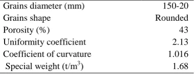
The cylindrical form was used in the present study due primarily to the adaptability and compliance of the cylinder coordinates with the physical conditions of radial flows problems. Semi cylindrical model allows the convergent (radial) flow towards the center of a well. The semi cylindrical physical model is of 6 and 3 meters in diameter and height, respectively. In 1 meter of the bottom is included a tank for required water supply during the experiments. The 2 meters above accommodates the porous media (aggregates) with a volume of about 28 m3. Fig. 1 illustrates a schematic of the laboratory model. The aggregates used in the physical model are course-grained. The specifications of model have been provided in Table 1.

Figure 1. Schematic of the physical model used in the study

Table 1. Specification of the aggregates used in the physical model 150-20

Grains diameter (mm)

Rounded Grains shape

43 Porosity (%)

2.13 Uniformity coefficient

1.016 Coefficient of curvature

1.68 (

t/m3 ) Special weight

(17)

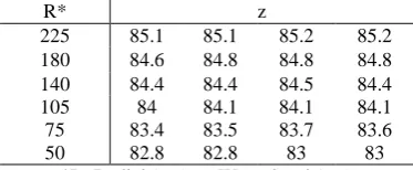
A total of 210 piezometers show the pressure changes in the model. For a precise piezometeric pressure reading, a number of scaled dials were used with millimeter precision. Since the experiment was performed on various levels of the water surface, the model was filled up to the intended level for every experiment and the numbers on four meters (mechanical and digital) were read, showing the flow volume that crossed through the pumps (V1). By looking at

the water surface profile on the glass view of the physical model, piezometeric pressure was read on the piezometers panel. After a few minutes, the pumps and stopwatches were turned off simultaneously and the number on the four counters were noted again (V₂). The tank was filled up to a determined depth. The considered depths were 52, 70, 85, 95,110, 120, 140, 150, 160 cm. After every experiment, the data were noted for different depths and levels. Table 2 and 3 show a sample of the data for the depth of 85 cm.

Figure 2. Position of piezometers on every section of the physical model

Table 2. Hydraulic specifications of the flow, measured for the depth of 85 cm Mean Flow Velocity (cm/s) Flow Rate

(cm/s) Water Level (cm)

Section Number Radial (cm) - 0.83 70.2 External Border 275 0.76 0.84 85.6 1 225 0.95 1.06 85.3 2 180 1.21 1.36 84.9 3 140 1.60 1.83 84.5 4 105 3.90 2.58 83.9 5 75 3.24 3.90 83.1 6 50 5.94 7.98 81.3 Internal Border 25

Table 3. Values of piezometeric pressure in different levels (z) for the depth of 85 cm z R* 85.2 85.2 85.1 85.1 225 84.8 84.8 84.8 84.6 180 84.4 84.5 84.4 84.4 140 84.1 84.1 84.1 84 105 83.6 83.7 83.5 83.4 75 83 83 82.8 82.8 50

(18)

In the physical models of parallel flows, the cross section is constant. So, the hydraulic gradient is calculated for successive points, while the cross section in the radial flows is variable. Base on this, in this study, the hydraulic gradient was calculated by the three following methods; difference of successive radii (R1-R2), (Method I); keeping constant the minimum radius (R1 -R_min), (Method II), and keeping constant the maximum radius (R₁-R_max), (Method III). The hydraulic gradient sample values (iobs) in the depth of 85 cm and level of 20 cm are shown in

Tables 4, 5 to 6 for the three methods.

Table 4. iobs values measured by the Method I in the depth of 85 cm and level of 20 cm

v(m/s) r(cm) R H ∆H ∆l

iobs *

0.009 225 202.5 85.1 0.5 45 0.011 0.012 180 160 84.6 0.2 40 0.005 0.016 140 122.5 84.4 0.4 35 0.011 0.022 105 90 84 0.6 30 0.02 0.032 75 62.5 83.4 0.6 25 0.024

* The observed hydraulic gradient (iobs) is obtained by the ratio of the difference between two successive points

(∆H = H1− H2) and the radial distance between them(∆l = R1− R2). Average radius was used in the

calculations(𝑅 = (𝑟1+ 𝑟2)⁄2), H1:The first point piezometeric pressure, H2:The second point piezometeric pressure,

R1: The first average radius, R2: The second average radius, H: Piezometeric pressure, R:radial, v: Velocity

Table 5. iobs values measured by the Method II in the depth of 85 cm and level of 20 cm

v(m/s) r(cm) R H ∆H ∆l

iobs *

0.023 225 137.5 85.1 2.3 175 0.013 0.024 180 115 84.6 1.8 130 0.013 0.026 140 95 84.4 1.6 90 0.017 0.028 105 77.5 84 1.2 55 0.021 0.032 75 62.5 83.4 0.6 25 0.024

* The observed hydraulic gradient (iobs) is obtained by the ratio between the piezometeric pressure difference of a

point and the minimum-radius point (∆H = H − Hmin) and the radial distance between them (∆l = R − Rmin)

Average radius was used in the calculations(𝑅 = (𝑟1+ 𝑟2) 2⁄ ); Hmin:The minimum-radius point piezometeric pressure, 𝑅:Average radius, Rmin: The minimum-radius point, H: Piezometeric pressure , r:Radial,v: Velocity

Table 6. iobs values measured by the Method III in the depth of 85 cm and level of 20 cm

v(m/s) r(cm) R H ∆H ∆l

iobs *

0.009 180 202.5 84.6 0.5 45 0.011 0.011 140 182.5 84.4 0.7 85 0.008 0.013 105 165 84 1.1 120 0.009 0.017 75 150 83.4 1.7 150 0.011 0.023 50 137.5 82.8 2.3 175 0.013

* The observed hydraulic gradient (iobs) is obtained by the ratio between the piezometeric pressure difference of a

point and the minimum-radius point (∆H = Hmax− H) and the radial distance between them (∆l = Rmax−

R)Average radius was used in the calculations(R = (r1+ r2) 2⁄ ), Hmax: The maximum-radius point piezometeric

pressure, R: Average radius, Rmax: The maximum-radius point, H: Piezometeric pressure , R:radial, v:Velocity

3 Results and discussion

(19)

and b coefficients were calculated in the binomial Forchheimer equations for different levels and depths. Table 7 shows a sample of a and b values for the levels of 20 and 35 cm and the depth of 52 cm. The results show that in contradiction to the basic Forchheimer equation, the nonlinear coefficient of b (the slope of the hydraulic gradient-velocity curve (i-v), which is a positive) obtains negative values (Table 7 and Fig. 3).

Table 7. The calculated value of Forchheimer a and b constant coefficients for the levels of 20 and 35 cm and the depth of 52 cm

B a

z

-7.310 1.311

20

-7.779 1.409

35

z: Water level (cm); a & b: The coefficients of Forchheimer equation

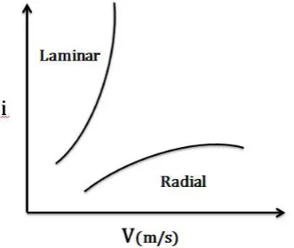
As seen previously, the hydraulic behaviors of parallel and radial flows are totally different. One of the differences is the constant and variable cross sections in parallel and radial flows. This declares the type of changes between hydraulic gradient and velocity of the flow along the way and the i-v curve form. On this basis, in the parallel flow, the flow’s cross section is constant along the way. So, the variations of hydraulic gradient are more pronounced than the velocity variations. However, in radial flow, the cross section of the flow is not constant along the way. So, the velocity variations are more than the pear hydraulic gradient variations. The i-v curve for the parallel flows (Forchheimer equation) is shown in the Fig. 3 which tends toward the orthogonal axis of the hydraulic gradient (i) and shows the higher variations of hydraulic gradient relative to the velocity in the parallel flows(v). However, in radial flows, the velocity variations are more significant than the hydraulic gradient variations and it is expected that the i-v curi-ve tends towards the horizontal i-velocity axis (Fig. 3).

Figure 3. The schematic velocity – hydraulic gradient (i-v) curve of the parallel and radial flow

(20)

independent variable (R) is also required in addition to the independent variable of velocity (v) and the dependent variable of hydraulic gradient (i). To provide the intended equation, some of the data related to the experimental readings for the depths of 52, 70, 85 and 95 cm and the levels of 20, 35, 55 and 80 cm were taken as regression data, and those related to the depths of 110, 120, 140, 150 and 160 cm and the levels of 20, 35, 55, 80, 105, 130 and 155 cm were taken as test or verification data. Therefore, the equations of (4), (5) and (6) were obtained for the methods I, II, III, respectively, in order to predict the hydraulic gradient ipre by regression data

(measured in various conditions in the laboratory, Tables 4, 5 and 6), including the hydraulic gradient(i), radius(R) and velocity (v) variables and using the common statistical software. The predicted hydraulic gradient, ipre, was calculated as a sample using these equations for the depth

of 85 and level of 20 cm, the values are provided in the Tables 8.

𝑖_𝑝𝑟𝑒 _{= 𝑣 −𝑎 + 𝑏𝑅}⁄ (4)

𝑖𝑝𝑟𝑒 = 𝑎𝑅−𝑏 𝑣⁄ (5)

𝑖𝑝𝑟𝑒 = 𝑉 ⁄ (𝑎 − 𝑏𝑅2 ) (6)

where ipre is the predicted hydraulic gradient, R is the average radius, V is the average velocity, and a and b are the constant coefficients.

Table 8. The values of ipre predicted by the Method I, II, III in the depth of 85 and level of 20 cm

v r R 𝒊𝒐𝒃𝒔 ipre 0.009 225 202.5 0.011 0.006 M eth o d

I _0.008 _0.005 ₁₆₀ ₁₈₀ _0.012 0.016 140 122.5 0.011 0.012 0.022 105 90 0.02 0.017 0.032 75 62.5 0.024 0.028 0.023 225 137.5 0.013 0.013 M eth o d

II 0.014 0.013 115 180 0.024 0.026 140 95 0.017 0.017 0.028 105 77.5 0.021 0.020 0.032 75 62.5 0.024 0.024 0.009 180 202.5 0.011 0.010 M eth o d II I 0.011 140 182.5 0.008 0.009 0.013 105 165 0.009 0.009 0.017 75 150 0.011 0.010 0.023 50 137.5 0.013 0.013

ipre:Predicted hydraulic gradient, iobs:Observed hydraulic gradient, R:Mean radius(cm), r: Radial(cm); v:

Velocity(m/sec)

(21)

hydraulic gradient by keeping the maximum radius constant.

Table 9. Variation percentage of a and b coefficients in the three methods

b a Variation percentage 0.236 0.671 Method I 0.173 0.294 Method II 0.301 0.128 Method III

In this study, Nash coefficient (E) and Root Mean Square (RMS) are used to measure the hydrological prediction ability as the equations (7) & (8).

(7)

𝐸 = 1 −∑ (𝑁𝑖(0)− 𝑁𝑖(𝑝))

2 𝑛

𝑖=1

∑𝑛 (𝑁_𝑖(0)− 𝑁_𝑚)2

𝑖=1

(8)

𝑅𝑀𝑆𝐸 = √∑ (𝑁𝑖(0)− 𝑁𝑖(𝑝))2

𝑛 𝑖=1

𝑛

In these equations, 𝑁_𝑖(0), 𝑁_𝑖(𝑝) and 𝑁_𝑚 are the observed, predicted and mean values, respectively, and n is the number of the data. The closer the E and RMSE to 1 and 0, respectively, the more suitable the behavior of the model or equation. Table 10 shows the values of E and RMSE to evaluate the three methods related to different depths and levels. According to the Table 10, the values of E and RMSE related to the Method III are closer to 1 and 0, respectively.

Table 10. The values of E and RMSE in the three Methods (I, I and III) E RMSE z Depth (III) (II) (I) (III) (II) (I) 0.9989 0.7143 0.4762 0.0007 0.0007 0.0118 20 52 0.9993 0.4140 0.5760 0.0007 0.0013 0.0123 35 52 0.9989 0.5138 0.3759 0.0005 0.0009 0.0082 20 70 0.9971 0.2139 0.5759 0.001 0.0007 0.0093 35 70 0.9452 0.3144 0.3762 0.0219 0.0004 0.0071 55 70 0.9991 0.7145 0.4763 0.00061 0.0008 0.0949 20 85 0.95125 0.6141 0.7760 0.0005 0.0005 0.0057 35 85 0.9300 0.7137 0.8758 0.00028 0.0007 0.0041 55 85 0.9776 0.7144 0.3762 0.00057 0.0004 0.0053 80 85 0.8943 0.5142 0.8761 0.0003 0.0002 0.0044 20 95 0.9416 0.3143 0.9762 0.0005 0.0003 0.8354 35 95 0.9971 0.6141 0.5760 0.0005 0.0002 0.8372 55 95 0.9743 0.7145 0.0763 0.000629 0.0003 0.0043 80 95

D: Depth (cm); z: Water level (cm); RMSE: Root Mean Square; E: Nash Coefficient

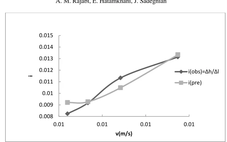
For example, the data in Table 6 for the Method III (Equation 6) is provided in Fig. 4 as a relationship between ipre and iobs values and the average velocity. The values of RMSE and E

obtained by Table 10 are, respectively, 0.0006 and 0.9991, showing the closeness of ipre values to

iobs values using the equation (6). Then this equation would be an appropriate equation for the

(22)

Figure 4. i-v curve for the depth of 85 cm and levels of 20 cm

In order to assess the consistency of the values obtained by the experimental results (observed values) with the values predicted by the equation (6), verification was performed by test data. For verification of the equation (6), the values of a and b coefficients should be determined for studied aggregates. Table 11 shows a and b coefficients and their average for the test data.

Table 11. a and b coefficients used in calculation of the gradient based on the equation (6) for the aggregates tested in this study

D z b a* 85 20 4.05×10-5 2.542 85 55 3.58×10-5 2.521 85 80 3.53×10-5 2.458 95 20 2.84×10-5 2.394 95 35 2.96×10-5 2.409 95 55 4.07×10-5 2.724 95 80 3.82×10-5 2.748 - - 3.546×10-5 2.542 Average

* a & b: the coefficients of Forchheimer equation; z: water level(cm); D: depth (cm)

By averaging the experimental coefficients of a and b and their substitution in the equation (6), a basic equation is obtained for the verification of the proposed equation for tested aggregates as follows:

(7)

𝑖 = 𝑉 ⁄ (2.542 − 3.546 × 10−5_𝑅2₎

In this equation, i is the hydraulic gradient, R is the average radius, and V is the average velocity.

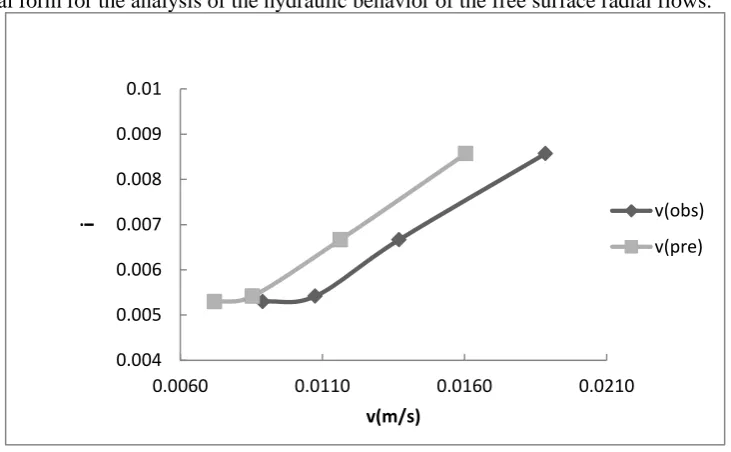
Using the hydraulic gradient values obtained by the Method III and the average radius (R), the velocity of the flow (vpre) was acquired according to the equation (7). Fig. 5 shows the relationship between the hydraulic gradient and the observed and predicted velocities and shows the acceptable consistency of the graphs. According to the Fig. 5, there is a small difference between the values of vobs (average velocity between every point and the most distant point from

the center of the well) and vpre (obtained by the equation 7). So, the equation (6) is an appropriate 0.008 0.009 0.01 0.011 0.012 0.013 0.014 0.015

0.01 0.01 0.01 0.01

i

v(m/s)

i(obs)=∆h/∆l

(23)

functional form for the analysis of the hydraulic behavior of the free surface radial flows.

Figure 5. i-v curve for the depth of 110 cm and the levels of 20 cm

4 Conclusions

Equations of fluids in porous media are very useful in designing the rockfill dams, diversion dams, gabions, breakwaters, and ground water reserves. The behaviors of the parallel and radial flows are totally different. Of importance among the differences is the constant and variable cross section of the flow in parallel and radial flows, respectively. This determines the type of variations between the flow velocity and hydraulic gradient along the way, and also variations in the profile of velocity-hydraulic gradient (i-v) curve. A new equation has to be developed which is applicable for the course grained porous media due to the negative coefficient of the nonlinear binomial Forchheimer equation in practical applications of the radial flows on the one hand, and the invalidity of the mentioned equation for the description of the free surface radial flows in the course grained porous media, on the other. Accordingly, in the present paper, a radial flow to the center of a well was modeled by developing a semi cylindrical physical model. Thereafter, different flow parameters were measured, including flow rate, hydraulic gradient, velocity, radial distance from the center of the model and various levels. Then, choosing a series of data as regression data, different equations were obtained for the prediction of hydraulic gradient by the three methods of difference of successive radii, keeping constant the minimum radius and keeping constant the maximum radius. The comparison of the attained the equations and verification of results obtained by them was shown that the functional form of the equation

i = V ⁄ (a − bR2₎_{is appropriate for the analysis of the hydraulic behavior of free surface radial}

flows. This study was performed on a bed with a predetermined grain size and flow rate and in the laboratory conditions. This phenomena is slightly different in nature than what has been observed in the study. This study can be carried out in a porous medium with different granulation, different flow rates and hydraulic gradients and compared to the results of this study. Also, changing the dimensions of the physical model and therefore the boundary conditions, can yield different results.

0.004 0.005 0.006 0.007 0.008 0.009 0.01

0.0060 0.0110 0.0160 0.0210

i

v(m/s)

v(obs)

(24)

5. References

1. Ahmed, N., Sunada, D.K.: Nonlinear flow in porous media. J. Hydra. Divi. ASCE. 95(6), 847-1857 (1969)

2. Bazargan, J., Zamanisabzi, H.: Application of New Dimensionless Number for Analysis of Laminar, Transitional and Turbulent Flow through Rock-fill Materials. Canadian Journal on Environmental, Construction and Civil Engineering. 2(7), 2011

3. Bazargan, J., Byatt, H.: A new method to supply water from the sea through rockfill intakes. Proceeding of 5th international conference on coasts, ports and marine structures (ICOPMAS), October 14-17, Ramsar, Iran, PP.276-279 (2002)

4. Bazargan, J., Shoaie, M.: Non-Darcy flow analysis of rockfill materials using gradually varied flow theory. Journal of Civil Engineering and Surveying, 44(2), 131-139 (2010)

5. Ferdos, F., Dargahi, B.: A study of turbulent flow in large-scale porous media at high Reynolds numbers. Part I: numerical validation, Journal of Hydraulic Research. 54 (6), 663-677 (2016 a)

6. Ferdos, F., Dargahi, B.: A study of turbulent flow in large-scale porous media at high Reynolds numbers. Part II: flow physics, Journal of Hydraulic Research, 54 (6), 678-691 (2016 b)

7. Hansen, Garga, V.K., Townsend, D.R.: Selection and application of a one-dimensional non-darcy flow equation for two dimensional flow through rockfill embankment. Can. Geotech. J.

33,223-232 (1995)

8. Sadeghian, J., Khayat Kholghi, M., Horfar, A., Bazargan, J.: Comparison of Binomial and Power Equations in Radial Non-Darcy Flows in Coarse Porous Media. JWSR Journal. 5 (1) 65- 75 (2013)

9. Li, B., Garga, V.K., Davies, M.H.: Relationship for non-Darcy flow in rockfill. J. Hydraul. Eng., ASCE. 124(2), 206-212 (1998)

10. Mc Whorter, D.B., Sunada, D.K.: Groundwater Hydrology and hydraulics. Water Resources Publication, Fort Collins, Colorado, USA, PP. 65-73 (1977)

11. Mc Corquodale J.A.: Finite Element Analysis of Non-Darcy Flow. Ph D Thesis, University of Windsor, Windsor, Canada (1970).

12. Sedghi-Asl, M., Rahimi, H., Farhoudi, J., Hoorfar A., Hartmann, S.: One-Dimensional Fully Developed Turbulent Flow through Coarse Porous Medium. Journal of Hydrologic Engineering. 19(7), 2014.

13. Nasser, M.S.S.: Radial Non-Darcy flow through porous media. Master of Applies science thesis, University of Windsor, Windsor, Canada (1970)

14. Reddy, N.B.: Convergence factors effect on non- uniform flow through porous media. IE(I) Journal.CV. 86, (2006)

15. Reddy, N.B., Roma Mohan Rao, P.: Effect of convergence on nonlinear flow in porous media.Hydr. Engrs ASCE. April 420-427 (2006)

16. Sadegian. J.: Nonlinear analysis of radial flow in coarse alluvial beds, Ph.D Thesis, College of Agriculture, University of Tehran, Iran (2013)

17. Das, B.M, Sobhan, K.: Principles of Geotechnical Engineering, Eighth Edition, SI , Publisher, Global Engineering: Christopher M. Shortt; Printed in the USA (2012)

18. Thiruvengadam, M., Pradip Kumar G.N.: Validity of forchheimer equation in radial flow through Coarse granular media. Journal of engineering mechanics, 123(7), (1997)

(25)

20. Ward, J.C.: Turbulent flow in porous media. J. Hydra. Div. ASCE. 95 (6), 1-11 (1964) 21. Wright D.E.: Seepage Patterns Arising from Laminar, Transitional and Turbulent Flow

(26)

J. Hydraul. Struct., 2017; 3(2): 22-31 DOI: 10.22055/jhs.2018.24654.1062

Three-dimensional numerical modeling of score hole in

rectangular side weir with finite volume method

Samira Ghotbi1 Azam Abdollahi2

Mehdi Azhdari Moghadam3

Abstract

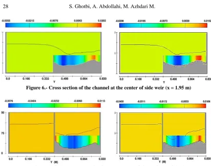
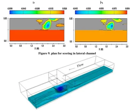
Local scouring in the downstream of hydraulic structures is one of the important issues in river and hydraulic engineering, which involves a lot of costs every year, so the prediction of the rate of scour is important in hydraulic design. Side weirs are the most important of hydraulic structures that are used in passing flow. This study investigates the scouring due to falling jet from side weir in downstream in side channel numerically. The simulation was done with finite volume method. The comparison of numerical and experimental results of flow fields shows agreement. Results show that from upstream to downstream of side weir located in side channel, scoring is increased and the dimensions of the scour hole in the downstream of the rectangular side weirs increase along it. In fact, at the downstream of the lower edge of side weirs in side channel, scouring has the greatest dimensions; in particular the depth.

Keywords: Scour, Side weir, Three-dimensional Modeling, Finite volume method.

Received: 08 October 2017; Accepted: 06 November 2017

1. Introduction

Side weirs are common hydraulic structures that are used to transfer water from the main canal to the side channel, these structures are used to control flood and divert temporary flow. So far, many studies have been conducted on the discharge coefficient ([1], to [4]) and changes in the geometry of these side weirs ([5], to [7]) in a fixed bed. G. Michellazo, in an experimental study investigated the effect of the moving bed in the main channel on the flow properties of rectangular side weir. Finally, the results showed that the side weir in the moving bed for deviating the flow is much more effective than in the fixed bed [8]. Scouring is a natural

1 _{Faculty of Civil Engineering, University of Sistan and Baluchestan, Zahedan, Iran,}

[email protected] (Corresponding author)

[email protected]

(27)

phenomenon due to water flow on erosion bed’s rivers and canals. Also local scouring is part of the morphological changes of the waterways, which is mainly due to various structures made by human [9]. Up to now, a lot of study has carried out on the local scoring in the downstream of the conserved bed. Farhoudi & Smith, examined the scour profiles in the downstream of hydraulic jump and presented the scour hole according to dimensionless profiles [10]. Balachandar et al., investigated the effect of a tail water depth on scour hole development on a loose bed of cohesion less sand material then provided diagrams for the development of the scour hole at different times [11]. The outflow of hydraulic structures is often as a jet that may causes significant changes in the topography of the river and surrounding these structures. It is caused substantial damages and environmental effects. The jet with high speed creates a great shear stress which often has a critical shear stress to start moving particles. Passing time, bed scour increases scour depth also reduces shear stress that causes a reduction the rate of scour [12]. With time, this leads to equilibrium a scour depth [13]. Equilibrating in the scour depth is an approximation phenomenon [11]. Jo Jong-Song, in a 2D numerical model investigate the local scour alteration in open channels of a tideland dike and concluded as the width of open channel between tideland dikes decreased, due to increased flow velocity, the scoured depth intensely increased [14]. M. Burkow, M. Griebel, investigate a 3D numerical simulation of fluid flow and sediment transport at rectangular obstacle. Results show the typical vortex system for the sediment transport and its interplay with shear stress and transport rates [15]. Török et al., offered a combined application of two bedload transport formulas that extends the application usage. Consequently more suitable simulation results [16].

Figure1. Flow pattern of falling jet in score hole

Sediment transmission and Problems concerning its caused existence challenge in hydraulic structures. This subject is studied by engineers and river morphologists. In recent years, hydraulic and sediment science have progressed vastly. For the first time Shields examined the threshold of sediment motion. He presented a diagram that is surveyed the stability of soil channel and rivers. There are several insight for estimating the dimension of scour hole in the downstream of hydraulic structures. Several analytical, experimental, and laboratory relationship has been proposed to determine the depth, width and length of scour hole ([17], [18]). One of the Relationships for estimating the depth of the scour hole in the downstream of Falling jet is Veronese [19]:

(1)

That q is flow rate and H1 is the height of the cascade. The above relation is very simple and

just using these two parameters, the depth of the scour hole can be calculated and the effect of

0.54 0.225

1

1.9

s

(28)

sediment properties is not considered. Another relationship to calculate the depth of scouring is given that In addition to the the above parameters, also the physical properties of the sediment, are considered [20].

(2)

g, dw and d, are Gravity acceleration, the depth of tail water depth, and the particle diameter index respectively which, according to their suggestion, is the same as the average particle diameter d50. According to the previews studies, Investigation of scouring in downstream of side wires is unprecedented. Thus in this research a numerical model of scouring due to falling jet from rectangular lateral side weir has been investigated. Although the prediction of scour depth and the estimation of the final shape of the bed by laboratory models seems reasonable, but from the point of view of cost and time, it is not affordable. Using a series of assumptions, the governing equations of the flow and sediment can be simplified. In this research, a three dimensional numerical model is used.

2. Mathematical modeling

In this research, mathematical simulation of flow over the rectangular side weir and sediment transport in the bed of side channel in downstream the side weir has been developed. For this purpose, finite volume (VOF) method has been used for numerical solution of equations. Rectangular cube cells grid has been used for the domain mesh generation. Selection of this grid is because of easy to generation, the proper order and less memory need.

3. Governing equations:

Sediment scouring models are sensitive to the turbulence model because the turbulence model directly affects the viscosity. Using viscosity, the shear stress is calculated locally. Also, for calculating the transport rate and erosion of the load, the local shear stress is used. The RNG turbulence model is mainly recommended for scouring modeling in this software [21] that used in this study. In the present study, following assumptions are used:

(a) An incompressible fluid (water) flows. (b) The pressure distributed hydrostatically.

(c) Flow is shallow enough thus Vertical accelerations be neglected. (d) The effects of wind and wave are ignored.

The governing equations for fluid flow in this study are the continuity and momentum equations that are presented below.

Mass continuity equation:

(3)

Where VF is the volume fraction of the flow, ρ is the fluid density, R is the coefficient of the

cylindrical or Cartesian coordinates in the equation,

R

DIF _{is Disturbance phrase, and}

R

SOR_{is the} mass source.

u

,

v

and

w

represent the velocity along x, y and z.

A

x ،

A

y _and

A

z _{Equal to the} fractions of the surface for flow along x, y and z. The first term on the right hand side of the

1 0.6 0.05 0.15

0.3 0.1

3.27 w

s

q H d

d

g d 

(

)

(

)

(

)

x

F x y z DIF SOR

uA

V

uA

R

vA

wA

R

t

x

y

z

x



_

_









(29)

above equation is related to the disturbances and defined as:

( ) ( ) ( ) x

DIF x y z

A

R A R A A

x x y y z z x





         

      (4)

And the second term on the right hand side of equation represents the change in density.

2

y

x x SOR

F

uA

vA

z

uA

R

V

P

wA

R

c

t

x

y

z



x





_

_



(5)

That P is the pressure and c is the velocity of the wave. The momentum equation in three directions in three dimensions are:

2

1 1

( )

y SOR

x y z x x x w s

F F F

A v R

u u u u P

uA vA wA G f b u u u

t V x y z  xV  x V 

 

 _  _  _  _ _{ }  _ _ _{ } _ _

 

 _    _  (6)

1 1

( )

y SOR

x y z y y y w s

F F F

A vu R

v v v v P

uA vA wA G f b v v v

t V x y z  xV  y V 

 

 _  _  _  _ _{ }  _ _ _ _ _ _

 

 _    _  (7)

1 1

( )

SOR

x y z z z z w s

F F

R

w w w w P

uA vA wA G f b w w w

t V x y z  z V 

 

 _  _  _  _{ }  _ _ _ _ _ _

 

 _    _  (8)

x

f

_،

f

_y

and

f

z _{parameters are the viscosity accelerations and}

G

x ،

G

y _and

G

z _are Volumetric accelerations and

b

x ،

b

y _and

b

z _{are Flow drops in permeable environments.}

4. Computational domain:

In order to validate the numerical model in this study, the experimental results of rectangular side weir were studied by Bagheri and Haydarpour [22], is used. The specifications of the hydraulic structure are as follows. The main channel was designed with a length of 3 meters and a width of 0.4 meters and a height of 35/0. The rectangular side weirs location is 1.8 meters from the beginning of the channel. The side weirs specifications is presented in the table below. The side channel is along the main channel with a same width to main channel. Bottom of the side channel has been covered with aggregate materials. Sediment height at the bottom of the side channel is 10 cm. The diameter of sediment aggregates in this study is equal to 0.005 mm and their density is 2650 kg / m3.

Table1. Specifications of side weir [22] (

m3/s )

inflow Length (cm) Height (cm)

0.042 30 15.4

Sediment characteristic parameters in the side channel are presented in table 2. The soil is cohesion less.

Table2. Specifications of sediment Bed loading Suspension coeff. Critical shields Bed

loading coeff. Angle (degree)

0.018 0.05 8 32

JHS, Vol. 3, Issue 2

Journal of Hydraulic Structures

Department of Civil Engineering

Shahid Chamran University of Ahvaz

In the name

of GOD

HYDRAULIC

STRUCTURES

CONTENTS

II

Aims and Scope

01

Investigating the vulnerability downstream

area of Taleghan dam due to dam failure

10 An experimental study on hydraulic

behavior of free-surface radial flow in

coarse-grained porous media

22 Three-dimensional numerical modeling of

score hole in rectangular side weir with

finite volume method

32 Experimental Study of the Effect of

Base-level fall at the Beginning of the Bend on

Reduction of Scour around a Rectangular

Bridge Pier Located in the 180 Degree

Sharp Bend

47 Developing optimal operating reservoir

rule-curves in drought periods

62 Finding the Causes and Evaluating Their

Impacts on Urmia Lake Crisis

‎

Using a

Comprehensive Water Resources

Simulation Model

Aims and Scope

General Information

Investigating the vulnerability downstream area of Taleghan

dam due to dam failure

Abstract

1. Introduction

2. Methodology

2.1. Study area

2.2 Physical characteristics of Taleghan river in Taleghan dam downstream

2.3 Determining boundary conditions

2.4 Discharge inflow

2.5 The risk taking theory due to dam failure

3. Results

4. Conclusion

References

An experimental study on hydraulic behavior of free-surface

radial flow in coarse-grained porous media

Abstract

1. Introduction

2 Materials and methods

3 Results and discussion

4 Conclusions

5. References

Three-dimensional numerical modeling of score hole in

rectangular side weir with finite volume method

Abstract

1. Introduction

1.9

2. Mathematical modeling

3. Governing equations:

Mass continuity equation:

R

R

u

v

w

A

A

A

(

)

(

)

(

)

uA

V

_

_

_

_

_

_

_

_

_