Investigating methods of estimating parameters in Cox model with two incorrectly specified random effects: A simulation study

(1)

INVESTIGATING METHODS OF ESTIMATING PARAMETERS IN COX

MODEL WITH TWO INCORRECTLY SPECIFIED RANDOM EFFECTS:

A SIMULATION STUDY

Olakiitan I. Adeniyi, Benjamin A. Oyejola

Department of Statistics, University of Ilorin, P.M.B 1515, Ilorin, Kwara State, Nigeria Corresponding Author: Olakiitan Adeniyi, [email protected]

ABSTRACT: Most observational data are found to be clustered. In situations like this, it is important to investigate whether there is variation in the predictor effect between the clusters. Such inter-cluster variation cannot be explained only by the heterogeneity of predictor effects across the cluster but also by heterogeneity of their baseline hazard risk. The aim of this work is to use the Penalized Partial likelihood method and Hierarchical likelihood to estimate the parameters of the model Cox model with two additive random effect when the random effect are wrongly specified via a simulation study for various cluster sizes, number of clusters, censoring percentages and magnitude of the random effect variance. The simulation study showed Hierarchical Likelihood estimates the random effects well than the Penalized Partial Likelihood but both methods estimates the fixed effect well.

KEYWORDS: Clustering, random effects models, censoring, penalized partial likelihood, hierarchical likelihood.

1. INTRODUCTION

Most observational, experimental and epidemiology data are found to be naturally clustered. Different form of clustering could be patients who are being treated in the same hospital or by the same medical practitioner. Another form of clustering that is of interest in survival analysis occur in situations where repeated, multiple or recurrence of an event is found in the same subject, such as repeated birth from a woman or recurrence of incidence of asthma in an asthmatic patient. In such cases the traditional proportional hazards model cannot be applied because of the inherent correlation of the event times. A possible solution to this problem is the use of conditional proportional hazards given the frailty which account for the inherent correlation between the event times within the subjects or the clusters ([Gut02]). Hierarchical data structure is of interest when the units at a lower level are nested in units of higher levels. Ignoring clustering or not adequately accounting for the hierarchical data structure may lead to biases of both regression coefficients and their standard errors. Also, standard errors of group-level

predictors may be underestimated if indeed clustering exists and it is ignored.

Many approaches have been applied to account for hierarchical data structure in survival analysis. The fixed effect model approach deals with hierarchical survival data by including the cluster as a categorical fixed effect in the model. This is achieved by arbitrarily setting one cluster as a reference group and a g-1 dummy variables representing the clusters can then be estimated using the Cox PH model where there are g clusters. This approach can be reasonable for a small number of clusters with no cluster-level predictors. But, with large number of clusters and small cluster size, the parameter estimation might become unstable and the efficiency of estimates may be affected (DMS09]). Also, estimate of the between-cluster effects cannot be made as they are absorbed into the cluster effects and inferences are specific to the actual clusters and not to the population of clusters that could be of interest.

The shared frailty approach assume that that subjects in a cluster share the same frailty which act proportionally on the baseline hazard, and this is why the model is called the shared frailty model. It was introduced by ([Cla78]) (who did not use the notion of ‘frailty’) and extensively studied in ([Hou00, TG00, D+02, D+03 and DJ04]). The lifetimes are assumed to be conditionally independent with respect to the shared (common) frailty. The limitation of this approach is that; it forces the unobserved factors to be the same within the cluster, which is generally not appropriate. Also, in most cases, shared frailty will only induce positive associations within the cluster. Whereas, in some situations, the survival times for subjects within the same cluster are negatively associated and the dependence between survival times within the cluster are based on marginal distributions of survival times.

(2)

model (i.e. a Cox model with two or more additive random effects at the cluster level) given as

(1)

Where and are jointly distributed and

represents respectively the random cluster and the random slope. is the observed predictor for subject

j in group i. This additive random effect model allows for the effect of a treatment at the individual level to vary between clusters (i.e. a random coefficient). 2. TWO ADDITIVE RANDOM EFFECTS COX

MODELS

Consider the case of a study of G-independent clusters i=1,…,G. Tij denotes the survival times for subject j

j=1,…,ni from group i and Cij is the corresponding right censoring time. Assuming the censoring times are independent of the survival times, the observations are and the censoring indicator . For each subject, the explanatory

variable is observed. The hazard for the jth subject

in the ith cluster with random group effect bi0 (i.e. hazard for the jth subject in the ith cluster that takes into account the correlation occurring in the data due to clustering with random cluster effects) is given by

(2)

where is the unspecified baseline hazard function at time t, β is the fixed effect parameter, is the random effect for the ith cluster. The random

effects are assumed to be independently and

identically distributed.

When variation between the cluster exists and is large, there is need to investigate whether there is variation in the predictor effect between the clusters. To achieve this, an extra random effect is added to model (2) which is the interaction between the observable and the unobservable variables. Then, the Cox model with two additive random effect models is expressed as;

(3)

where bi1 is the random predictor effect also known as

random coefficient or random interaction. The random effects are assumed to follow a multivariate normal distribution with mean 0 and a variance-covariance matrix Σ, with

.

The variance of the bi0 represents the heterogeneity

between the clusters of the overall baseline hazard and the variance of bi1 is the heterogeneity between clusters of the overall effect β1. If the variance is

null, then the observations from the same cluster are independent. A larger variance indicates greater heterogeneity across clusters and a greater correlation of the survival times for subjects belonging to the same cluster. A null implies no heterogeneity of the effect over clusters.

Given the random effects , observations

within cluster i are assumed to be independent. The full marginal log likelihood function for cluster i is given as;

The conditional likelihood function for cluster i is

(4)

where

Assuming the conditional independence of observation within a cluster and independence between clusters, the overall marginal likelihood function can be written as,

(5)

where

When the correlation structure for the two random effects is modelled by , we have

(3)

Hence, we obtain for :

With the cumulative hazard

function and

the conditional cumulative hazard function and and

The marginal log-likelihood in (5) cannot be used as it were to estimate the parameters of model (3) because of unspecified parameter of the baseline hazard which depends on integrations that cannot be solved analytically.

The focus of this paper is to investigate the methods of estimating the parameter of Cox model with two additive random effects given in (3) when the random effects are assumed be correlated but are wrongly specified. The random effects are assumed to follow a multivariate normal distribution with mean 0 and a variance-covariance matrix Σ,

with

. The covariance parameter

of the random effects is not assumed to be zero but wrongly assumed to be zero in estimating the parameters.

2.1. The Penalized Partial Likelihood

This estimation procedure was proposed by ([RP00]). ([RP00]) followed ([BC93]) in their approach for GLMM with normal random effects and applied Laplace’s method for integral approximation to (4) which leads to the approximate marginal log-likelihood by

(6)

where

If both Σ were known and were considered

fixed effects parameters, then the second line in (6) is penalized Cox full log likelihood ([Gre87]), while the last term in (6) is the penalty term penalizing for extreme values and , and are set of

parameters and a penalty term, it turns out that it can be maximized using penalized fixed effects partial likelihood (PPL),

where are the risk sets.

The estimation procedure is implemented in the coxme package for R software developed by ([The18]). ([ES12]) compare methods for fitting Cox model with two additive random effects using a simulated data built on real data set from veterinary science field.

2.2. Hierarchical Likelihood

The hierarchical likelihood approach was proposed by ([HLS01]) and can handle shared and nested frailty models with gamma and log-normal distributions. Given the common unobserved frailty for the ith unit

zi, the conditional hazard function is of the form

(4)

for the fixed covariates . The h-likelihood for

frailty model is defines by

where

is the sum of conditional log densities for tij and δij given zi, and

is the sum of log densities for

v

_i



log

u

_iwith parameter α. is a linear predictor for

the hazards and the baseline cumulative hazard function is given as;

Ha et al. ([HLS01]) proposed the use of the profile h-likelihood with eliminated, given by

where

does not depend on and

Are solutions of the estimating equations,

for k=1,…,l. is the number of events at and

is the risk set at

.

This estimation procedure is implemented in the frailtyHL package in R software ([HNL12).

3. PARAMETER SETTING OF THE SIMULATION STUDY

In order to investigate the Penalized Partial Likelihood and the Hierarchical likelihood, simulation studies from model (1.3) were conducted (with independent or correlated random effects). The magnitude of the heterogeneity variances set at σi0

2

=2, σi1

2_{=0.5; σ} i0

2

=0.5, σi1

2_{=0.25; σ} i0

2_{=0.25, σ} i1

2

=0.025, for large, moderate and small variances respectively. The number of clusters and cluster sizes were varied to have the same number of cluster and cluster size (G=10, g=10); (G=100, g=5); (G=10, g=100), more cluster with fewer cluster size and fewer cluster with more cluster size. The specified censoring rates were 0%, 20%, 50% and 90%. The parameters of the fixed effects were set at β1=-1 for the categorical covariate

and β2=1 for the continuous covariate in both the

independent and correlated random effects. Gompertz baseline hazard distribution was used in generating the survival time with shape and scale parameter set at 0.1 and 0.05 respectively. 1000 observations were generated from the model using R version 3.4.4 software and the approach given in the package ‘simsurv’ by Brilleman ([Bri18]).

The performances of the estimation procedures were investigated based on bias, absolute bias, as well as mean square error (MSE) of the fixed and the random effect estimates. Let



ˆ

be the estimated parameter of



, then the

,

4. RESULTS OF THE SIMULATION

In the simulation study, the penalized partial likelihood did not show convergence problems but the Hierarchical likelihood did not reach convergence. The fixed effects were well estimated by both procedures. The result of the simulation studies are summarized in Tables 1-8.

4.1. Effect of the Censoring Rate

(5)

Table 1: Means of fixed effect parameter estimates according to the number of clusters (G), clusters sizes (g), magnitude of variance and censoring percentages based on incorrectly specified random effects models

Over 1000 Simulated Data sets

Ce

n

so

rin

g

%

β1= -1.0 β2= 1.0

G 10 100 10 10 100 10

g 10 5 100 10 5 100

Method Mean Mean

Large Variance

0% PPL -1.0959 -1.0029 -0.9732 1.0270 0.9904 0.9981

HL -1.1038 -0.9844 -0.9745 1.0424 1.0034 0.9992

20% PPL -0.9391 -0.9910 -0.9973 0.9903 0.9527 0.9867

HL -0.9417 -0.9729 -0.9993 1.0022 0.9627 0.9883

50% PPL -0.9452 -0.9156 -0.9778 0.9483 0.8415 0.9917

HL -0.9469 -0.9006 -0.9802 0.9568 0.8497 0.9938

90% PPL -0.8434 -0.6619 -0.8791 0.8273 0.6151 0.9402

HL -0.8975 -0.6572 -0.8875 0.8585 0.6120 0.9470

Moderate Variance

0% PPL -1.0057 -1.0361 -1.0030 1.0169 0.9811 0.9983

HL -0.9899 -0.9961 -1.0044 1.0291 1.0036 0.9999

20% PPL -1.0069 -1.0078 -0.9900 1.0055 0.9532 1.0029

HL -0.9963 -0.9667 -0.9915 1.0184 0.9720 1.0049

50% PPL -0.9810 -0.9524 -0.9990 0.9570 0.9009 0.9892

HL -0.9740 -0.9203 -1.0019 0.9719 0.9159 0.9924

90% PPL -0.7254 -0.8729 -0.9162 0.9298 0.7600 0.9378

HL -0.9933 -0.8692 -0.9272 0.9133 0.7653 0.9464

Small Variance

0% PPL -1.0272 -0.9976 -0.9950 1.0178 0.9990 0.9999

HL -1.0066 -0.9696 -0.9961 1.0245 1.0058 1.0019

20% PPL -1.0384 -1.0130 -0.9972 0.9920 0.9808 0.9982

HL -1.023 -0.9855 -0.9979 1.0005 0.9855 0.9999

50% PPL -0.9909 -0.9835 -1.0186 0.9911 0.9497 0.9804

HL -0.9773 -0.9578 -1.0195 1.0014 0.9517 0.9824

90% PPL -1.0933 -0.9057 -0.9828 0.9951 0.8530 0.9732

HL -1.161 -0.8977 -0.9847 1.0155 0.8564 0.9765

Table 2: Means of random effect parameter estimates according to the number of clusters (G), clusters sizes (g), magnitude of variance and censoring percentages based on incorrectly specified random effects models

Ce

n

so

rin

g

%

G 10 100 10 10 100 10

g 10 5 100 10 5 100

Large Variance

σ01=2 σ12=0.5

0% PPL 2.3701 2.0907 2.1142 0.1958 0.2114 0.2317

HL 2.5664 2.0541 1.9457 0.5676 0.5372 0.5256

20% PPL 2.2544 2.0251 2.0792 0.2082 0.1895 0.2161

HL 2.2957 1.9951 1.8885 0.5958 0.4859 0.5046

50% PPL 2.0322 1.6453 2.1814 0.2420 0.1669 0.1961

HL 1.9840 1.6146 2.0436 0.7195 0.4675 0.4581

90% PPL 2.0989 0.9424 1.8404 0.5360 0.2779 0.1816

HL 3.1139 0.9414 1.8404 2.0010 0.4847 0.4774

σ02=0.5 σ12=0.25

0% PPL 0.6595 0.6801 0.6538 0.1280 0.0979 0.1087

HL 0.6026 0.6216 0.4913 0.4497 0.4179 0.2606

20% PPL 0.7922 0.5902 0.6504 0.1200 0.1025 0.1119

HL 0.7364 0.5443 0.5032 0.4170 0.3893 0.2727

50% PPL 0.5805 0.5119 0.6076 0.1314 0.1010 0.0957

HL 0.5524 0.4740 0.4985 0.4553 0.3774 0.2468

90% PPL 1.0783 0.3736 0.6219 0.9771 0.1274 0.1205

HL 1.2091 0.3590 0.5539 1.3534 0.3468 0.3768

Small Variance σ0

2

=0.25 σ1 2

=0.025

0% PPL 0.3119 0.2856 0.3236 0.0394 0.0310 0.0101

HL 0.3008 0.2732 0.2894 0.1417 0.1128 0.0349

20% PPL 0.3242 0.2751 0.3240 0.0481 0.0380 0.0131

HL 0.3158 0.2663 0.2906 0.1655 0.1099 0.0451

50% PPL 0.2783 0.2573 0.2951 0.0946 0.0645 0.0139

HL 0.2679 0.2611 0.2745 0.3244 0.1294 0.0467

90% PPL 0.4703 0.2067 0.3109 0.2510 0.1212 0.0298

(6)

Table 3: Bias of fixed effect parameter estimates according to the number of clusters (G), clusters sizes (g), magnitude of variance and censoring percentages based on incorrectly specified random effects models

Ce

n

so

rin

g

%

β1= -1.0 β2= 1.0

G 10 100 10 10 100 10

g 10 5 100 10 5 100

Large Variance

0% PPL -0.0959 -0.0029 0.0268 0.0270 -0.0096 -0.0019

HL -0.1038 0.0156 0.0255 0.0424 0.0034 -0.0008

20% PPL 0.0609 0.0090 0.0027 -0.0097 -0.0473 -0.0133

HL 0.0583 0.0271 0.0007 0.0022 -0.0373 -0.0117

50% PPL 0.0548 0.0844 0.0222 -0.0517 -0.1586 -0.0083

HL 0.0531 0.0994 0.0198 -0.0432 -0.1504 -0.0062

90% PPL 0.1566 0.3351 0.1209 0.4473 -0.3850 -0.0598

HL 0.1025 0.3428 0.1125 -0.1415 -0.3880 -0.0530

0% PPL -0.0057 -0.0362 -0.0030 0.0169 -0.0189 -0.0017

HL 0.0101 0.0039 -0.0044 0.0291 0.0036 -0.0001

20% PPL -0.0069 -0.0078 0.0010 0.0055 -0.0468 0.0029

HL 0.0037 0.0333 0.0085 0.0184 -0.0280 0.0049

50% PPL 0.0190 0.0476 0.0010 -0.0430 -0.0991 -0.0108

HL 0.0260 0.0797 -0.0019 -0.0281 -0.0841 -0.0076

90% PPL 0.2746 0.1271 0.0838 -0.0702 -0.2400 -0.0622

HL 0.0067 0.1308 0.0728 -0.0867 -0.2347 -0.0536

Small Variance

0% PPL -0.0272 0.0024 0.0050 0.0178 -0.0010 -0.0001

HL -0.0066 0.0304 0.0039 0.0245 0.0058 0.0016

20% PPL -0.0384 -0.0130 0.0028 -0.0071 -0.0198 -0.0018

HL -0.0230 0.0145 0.0021 0.0005 -0.0145 -5.2E-05

50% PPL 0.0092 0.0165 -0.0186 -0.0090 -0.0503 -0.0196

HL 0.0227 0.0422 -0.0195 0.0014 -0.0483 -0.0176

90% PPL -0.0933 0.0943 0.0172 -0.0050 -0.1470 -0.0268

HL -0.1610 0.1023 0.0153 0.0155 -0.1436 -0.0235

Table 4: Bias of random effect parameter estimates according to the number of clusters (G), clusters sizes (g), magnitude of variance and censoring percentages based on incorrectly specified random effects models

Ce

n

so

rin

g

%

G 10 100 10 10 100 10

g 10 5 100 10 5 100

Large Variance

σ01=2 σ12=0.5

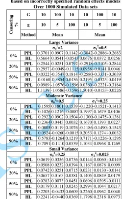
0% PPL 0.3701 0.0907 0.1142 -0.3042 -0.2886 -0.2683

HL 0.5664 0.0541 -0.0543 0.0676 0.0372 0.0256

20% PPL 0.2544 0.0251 0.0792 -0.2918 -0.3105 -0.2844

HL 0.2957 -0.0049 -0.1115 0.0958 -0.0141 0.0046

50% PPL 0.0322 -0.3547 0.1814 -0.2580 -0.3331 -0.3039

HL -0.0160 -0.3854 0.0436 0.2195 -0.0325 -0.0419

90% PPL 0.0989 -1.0576 -0.1596 0.0360 -0.2221 -0.3184

HL 1.1139 -1.0586 -0.1596 1.5010 -0.0153 -0.0226

σ02=0.5 σ12=0.25

0% PPL 0.1595 0.1801 0.1539 -0.1220 -0.1521 -0.1413

HL 0.1026 0.1216 -0.0087 0.1997 0.1679 0.0106

20% PPL 0.2922 0.0902 0.1504 -0.1300 -0.1475 -0.1381

HL 0.2364 0.0443 0.0032 0.1670 0.1393 0.0227

50% PPL 0.0805 0.0119 0.1076 -0.1186 -0.1490 -0.1543

HL 0.0524 -0.0260 -0.0015 0.2053 0.1274 -0.0032

90% PPL 0.5783 -0.1264 0.1219 0.7171 -0.1226 -0.1295

HL 0.7091 -0.1410 0.0539 1.1034 0.0968 0.1269

2

=0.25 σ1 2

=0.025

0% PPL 0.0619 0.0356 0.0736 0.0144 0.0060 -0.0149

HL 0.0508 0.0232 0.0394 0.1167 0.0878 0.0099

20% PPL 0.0742 0.0251 0.0715 0.0231 0.0130 -0.0141

HL 0.0657 0.0163 0.0381 0.1405 0.0849 0.0179

50% PPL 0.0283 0.0073 0.0451 0.0696 0.0395 -0.0111

HL 0.0179 0.0111 0.0245 0.2994 0.1044 0.0217

90% PPL 0.2203 -0.0433 0.0609 0.2260 0.0962 0.0048

(7)

Table 5: Absolute Bias of fixed effect parameter estimates according to the number of clusters (G), clusters sizes (g), magnitude of variance and censoring

percentages based on incorrectly specified random effects models Over 1000 Simulated Data sets

Ce

n

so

rin

g

%

β1= -1.0 β2= 1.0

G 10 100 10 10 100 10

g 10 5 100 10 5 100

Large Variance

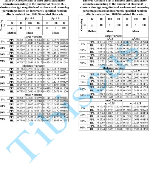
0% PPL 0.3081 0.1040 0.2064 0.1397 0.0573 0.0349

HL 0.3131 0.1042 0.2065 0.1442 0.0574 0.0348

20% PPL 0.3208 0.1150 0.1834 0.1641 0.0660 0.0406

HL 0.3266 0.1161 0.1842 0.1647 0.0620 0.0403

50% PPL 0.3622 0.1495 0.1940 0.1758 0.1612 0.0395

HL 0.3603 0.1602 0.1947 0.1743 0.1542 0.0395

90% PPL 0.7105 0.3902 0.2445 0.4473 0.3850 0.1077

HL 0.7097 0.3949 0.2417 0.4534 0.3380 0.1044

0% PPL 0.1882 0.0963 0.1245 0.1373 0.0615 0.0287

HL 0.2024 0.0938 0.1249 0.1397 0.0612 0.0286

20% PPL 0.2437 0.1030 0.1457 0.1399 0.0744 0.0332

HL 0.2523 0.1044 0.1459 0.1426 0.0678 0.0334

50% PPL 0.3240 0.1444 0.1470 0.1777 0.1218 0.0429

HL 0.3239 0.1553 0.1473 0.1792 0.1098 0.0427

90% PPL 0.9806 0.2584 0.2356 0.4818 0.2704 0.1150

HL 0.7504 0.2640 0.2383 0.4528 0.2671 0.1120

Small Variance

0% PPL 0.2067 0.0820 0.0599 0.1115 0.0534 0.0285

HL 0.2080 0.0823 0.0600 0.1185 0.0567 0.0288

20% PPL 0.2051 0.1012 0.0773 0.1293 0.0687 0.0387

HL 0.2066 0.1005 0.0781 0.1332 0.0680 0.0386

50% PPL 0.2732 0.1169 0.0818 0.1920 0.0779 0.0498

HL 0.2722 0.1193 0.0821 0.1978 0.0742 0.0494

90% PPL 0.7167 0.2457 0.1775 0.3987 0.1870 0.1216

HL 0.7540 0.2478 0.1787 0.4033 0.1863 0.1207

Table 6: Absolute Bias of random effect parameter estimates according to the number of clusters (G), clusters sizes (g), magnitude of variance and censoring

percentages based on incorrectly specified random effects models Over 1000 Simulated Data sets

Ce

n

so

rin

g

%

G 10 100 10 10 100 10

g 10 5 100 10 5 100

Large Variance

σ01=2 σ12=0.5

0% PPL 0.9016 0.2775 0.8614 0.3403 0.2954 0.2704

HL 1.1151 0.2844 0.7692 0.4414 0.1919 0.2019

20% PPL 0.9810 0.3439 0.8164 0.3412 0.3137 0.2844

HL 1.0548 0.3412 0.7654 0.4975 0.2069 0.1927

50% PPL 1.0525 0.4522 0.8029 0.3769 0.3385 0.3056

HL 0.9990 0.4723 0.7294 0.6066 0.2665 0.1985

90% PPL 2.170 1.2018 0.8648 0.7271 0.3859 0.3458

HL 3.0996 1.2261 0.8664 2.0277 0.5034 0.3440

σ02=0.5 σ12=0.25

0% PPL 0.3598 0.2012 0.3003 0.2090 0.1586 0.1413

HL 0.3307 0.1583 0.2046 0.3782 0.2030 0.0109

20% PPL 0.4453 0.1438 0.2811 0.1900 0.1573 0.1419

HL 0.3998 0.1232 0.1936 0.3532 0.2168 0.1175

50% PPL 0.4086 0.1486 0.2501 0.2225 0.1834 0.1593

HL 0.3871 0.1448 0.1837 0.4068 0.2438 0.1281

90% PPL 1.0354 0.3673 0.3049 1.0919 0.2175 0.1736

HL 1.1539 0.3618 0.2842 1.3774 0.3251 0.2741

2

=0.25 σ1 2

=0.025

0% PPL 0.1934 0.0791 0.1286 0.0464 0.0326 0.0169

HL 0.1914 0.0734 0.1084 0.1388 0.1013 0.0228

20% PPL 0.2063 0.0805 0.1358 0.0545 0.0400 0.0174

HL 0.1965 0.0814 0.1228 0.1603 0.0997 0.0311

50% PPL 0.2326 0.0409 0.1322 0.0954 0.0631 0.0188

HL 0.2207 0.0890 0.1227 0.3217 0.1228 0.0393

90% PPL 0.4977 0.2347 0.1635 0.2642 0.1259 0.0369

(8)

Table 7: Mean square error (MSE) of fixed effect parameter estimates according to the number of clusters

(G), clusters sizes (g), magnitude of variance and censoring percentages based on incorrectly specified random effects models Over 1000 Simulated Data sets

Ce

n

so

rin

g

%

β1= -1.0 β2= 1.0

G 10 100 10 10 100 10

g 10 5 100 10 5 100

Large Variance

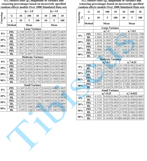
0% PPL 0.2789 0.0351 0.1295 0.0639 0.0097 0.0039

HL 0.2938 0.0352 0.1295 0.0707 0.0093 0.0039

20% PPL 0.3297 0.0394 0.1003 0.0800 0.0134 0.0054

HL 0.3385 0.0394 0.1011 0.0814 0.0121 0.0053

50% PPL 0.3893 0.0684 0.1264 0.1019 0.0648 0.0057

HL 0.3877 0.0771 0.1272 0.0995 0.0599 0.0056

90% PPL 1.5217 0.4740 0.2058 0.6224 0.3473 0.0347

HL 1.5787 0.4857 0.2036 0.6425 0.3510 0.0324

0% PPL 0.1138 0.0297 0.0454 0.0581 0.0126 0.0028

HL 0.1307 0.0282 0.0456 0.0617 0.0124 0.0028

20% PPL 0.1812 0.0321 0.0634 0.0684 0.0168 0.0032

HL 0.1900 0.0328 0.0636 0.0703 0.0139 0.0033

50% PPL 0.3437 0.0651 0.0701 0.0951 0.0429 0.0061

HL 0.3439 0.0736 0.0706 0.0963 0.0364 0.0061

90% PPL 12.1891 0.2273 0.1748 0.8101 0.1968 0.0413

HL 1.7518 0.2332 0.1792 0.6703 0.1919 0.0393

Small Variance

0% PPL 0.1367 0.0212 0.0115 0.0410 0.0089 0.0025

HL 0.1394 0.0232 0.0115 0.0442 0.0097 0.0029

20% PPL 0.1308 0.0317 0.0177 0.0509 0.0156 0.0051

HL 0.1382 0.0315 0.0180 0.0535 0.0156 0.0050

50% PPL 0.2216 0.0433 0.0217 0.1060 0.0191 0.0071

HL 0.2230 0.0455 0.0218 0.1114 0.0181 0.0069

90% PPL 1.8172 0.1960 0.0987 0.5370 0.1089 0.0442

HL 2.1459 0.1948 0.1006 0.6271 0.1082 0.0434

Table 8: Mean square error (MSE) of random effect parameter estimates according to the number of clusters

(G), clusters sizes (g), magnitude of variance and censoring percentages based on incorrectly specified random effects models Over 1000 Simulated Data sets

Ce

n

so

rin

g

%

G 10 100 10 10 100 10

g 10 5 100 10 5 100

Large Variance

σ01=2 σ12=0.5

0% PPL 3.2051 0.2525 2.7146 0.2782 0.2010 0.1700

HL 4.5605 0.2615 2.0351 0.6359 0.1213 0.1309

20% PPL 4.0138 0.3895 2.1729 0.2867 0.2275 0.1852

HL 4.6575 0.3849 1.7821 0.8961 0.1286 0.1233

50% PPL 3.3998 0.6019 2.1629 0.3304 0.2645 0.2069

HL 2.9806 0.6548 1.9612 1.5105 0.2085 0.1215

90% PPL 30.9137 3.5514 2.2729 3.6840 0.3951 0.2758

HL 147.6017 3.6202 2.4334 54.0134 0.8002 0.3881

σ02=0.5 σ12=0.25

0% PPL 0.3930 0.1142 0.3211 0.1358 0.0621 0.0474

HL 0.3261 0.0759 0.1205 0.7889 0.1359 0.0415

20% PPL 0.6921 0.0706 0.2738 0.0874 0.0635 0.0470

HL 0.5711 0.0512 0.1249 0.5632 0.1355 0.0496

50% PPL 0.7429 0.0774 0.2066 0.1292 0.0813 0.0584

HL 0.6742 0.0758 0.1089 0.8220 0.2049 0.0579

90% PPL 8.3092 0.4244 0.3567 37.4745 0.1080 0.0762

HL 10.8675 0.4162 0.2991 16.3179 0.3453 0.2991

2

=0.25 σ1 2

=0.025

0% PPL 0.1221 0.0204 0.0642 0.0108 0.0035 0.0007

HL 0.1143 0.0175 0.0425 0.1243 0.0389 0.0019

20% PPL 0.1759 0.0219 0.0594 0.0161 0.0087 0.0011

HL 0.1727 0.0227 0.0467 0.1593 0.0404 0.0036

50% PPL 0.1756 0.0227 0.0711 0.0570 0.0179 0.0009

HL 0.1695 0.0247 0.0570 0.7656 0.0661 0.0055

90% PPL 1.5902 0.1478 0.1123 1.7054 0.1100 0.0063

(9)

4.2. Effect of the Magnitude of Variance

The bias, absolute bias and the MSE of both the fixed and random effect decreased as the magnitude of variance decreased for three methods of parameter estimation along this three different variance settings, this was the case for all the different censoring rates and the number of units considered.

4.3. Effect of the Number of Units

The bias, absolute bias and the mean square error (MSE) of the fixed effects parameter decreases with increasing samples size, the situation is opposite for the random effect parameter as the absolute bias and the MSE increases with increasing sample size. This was the case for the different censoring rate and the magnitude of variance considering three methods of estimation.

In estimating the random effect parameter, the HL gives a closer value to the true parameter specified compared to PPL.

5. CONCLUSION

The random effect of the additive random effects in the Cox model, with a random cluster effect and a random interaction were incorrectly specified and the performance of penalized partial likelihood and Hierarchical likelihood were investigated varying the cluster sizes, number of cluster, censoring percentages and the magnitude of the random effect variance. The performance of the estimation procedures were examined by simulating different data set that has these criteria could be present in real life data.

The estimation procedures estimated the fixed effect well under incorrectly specified random effects but Hierarchical likelihood gave a better estimate of the random effect than the Penalized partial likelihood. To this end, the Hierarchical likelihood is to be preferred when it is not known that the random effects are correlated if the interest is on the random effects than the fixed effect, but if the interest is estimating the fixed effect, both the Penalized partial likelihood and the Hierarchical likelihood could be used but the Penalized partial likelihood is computationally less intensive compared to Hierarchical likelihood.

LIMITATION OF THE STUDY

The study only implore simulated data set as there is no one dataset that could have all the varying criteria considered in this work.

REFERENCES

[Bri18] Brilleman S. – ‘simsurv’. A package for

simulating survival times. R package

version 0.2.2,

https://github.com/sambrilleman/simsurv, 2018.

[BC93] Breslow N., Clayton D. – Approximate inference in generalized linear models. Journal of the American Statistical Association, 88: 9-25, (1993).

[Cla78] Clayton D. – A model for association in bivariate life tables and its application in epidemiological studies of familial tendency in chronic disease incidence. Biometrika 65, 141- 151, (1978).

[DJ04] Duchateau L., Janssen P. – Penalized partial likelihood for frailties and smoothing splines in time to ﬁrst insemination models for dairy cows.

Biometrics 60, 608 – 614, 2004.

[DJ08] Duchateau L., Janssen P. – The Frailty Model. New York Springer-Verlag., 2008.

[DMS09] Dohoo I., Martin W., Stryhn H. –

Veterinary Epidemiologic Research. 2nd edition, Charlottetown, VER – Inc, 2009. [D+02] Duchateau L., Janssen P., Lindsey P.,

Legrand C., Nguti R., Sylvester R. –

The shared frailty model and the power for heterogeneity tests in multicenter trials. Computational Statistics & Data Analysis, 40: 603-620, 2002.

[D+03] Duchateau L., Janssen P., Kezic I., Fortpied C. – Evolution of recurrent asthma event rate over time in frailty models. Journal of the Royal Statistical Society (B) 52, 355 – 363, 2003.

[ES12] Elghafghuf A., Stryhn H. – Comparison of methods for fitting Cox models with random herd and treatment-by-herd effects. The 12th Islamic Countries Conference on Statistical Sciences. 23, 367-374, 2012.

(10)

model. International Statistical 55, 245-259, 1987.

[Gut02] Gutierrez R. G. – Parametric Frailty and Shared Frailty Survival Models. The Stata Journal. 2(1): 22-44, 2002.

[Hou00] Hougaard P. – Analysis of Multivariate Survival Data. Springer-Verlag, 2000. [HLS01] Ha I. D., Lee Y., Song J. K. –

Hierarchical likelihood approach for frailty models. Biometrika, 88: 233-243 2001.

[HNL12] Ha I. D., Noh M., Lee Y. – ‘FrailtyHL’:

Frailty models using h-likelihood. URL

http://CRAN.R-project.org/package=frailtyHL. R

package version 1.1 28, 30, 2012.

[RP00] Ripatti S., Palmgren J. – Estimation of multivariate frailty models using penalized partial likelihood. Biometrics, 56: 1016-1022, 2000.

[The18] Therneau T. – ‘coxme’. A package for

mixed effects Cox models. R package version 2.2-7, URL http://cran.r-project.org/web/packages/coxme/. 2018. [TG00] Therneau T., Grambsch P. – Modelling

Survival Data, Extending the Cox model.

New York: Springer. 2000.

[Wie10] Wienke A. – Frailty Models in Survival Analysis. Chapman & Hall/CRC. 2010. [XB96] Xue X., Brookmeyer R. – Bivariate