https://doi.org/10.5194/wes-2-547-2017
© Author(s) 2017. This work is distributed under the Creative Commons Attribution 3.0 License.
Using wind speed from a blade-mounted flow sensor for
power and load assessment on modern wind turbines
Mads M. Pedersen, Torben J. Larsen, Helge Aa. Madsen, and Gunner Chr. Larsen
Wind Energy Department, Technical University of Denmark, Frederiksborgvej 399, 4000 Roskilde, Denmark
Correspondence to:Mads M. Pedersen (mmpe@dtu.dk)
Received: 19 May 2017 – Discussion started: 14 June 2017
Revised: 11 October 2017 – Accepted: 12 October 2017 – Published: 20 November 2017
Abstract. In this paper an alternative method to evaluate power performance and loads on wind turbines using a blade-mounted flow sensor is investigated. The hypothesis is that the wind speed measured at the blades has a high correlation with the power and loads such that a power or load assessment can be performed from a few hours or days of measurements.
In the present study a blade-mounted five-hole pitot tube is used as the flow sensor as an alternative to the conventional approach, where the reference wind speed is either measured at a nearby met mast or on the nacelle using lidar technology or cup anemometers. From the flow sensor measurements, an accurate estimate of the wind speed at the rotor plane can be obtained. This wind speed is disturbed by the presence of the wind turbine, and it is therefore different from the free-flow wind speed. However, the recorded wind speed has a high corre-lation with the actual power production as well as the flap-wise loads as it is measured close to the blade where the aerodynamic forces are acting.
Conventional power curves are based on at least 180 h of 10 min mean values, but using the blade-mounted flow sensor both the observation average time and the overall assessment time can potentially be shortened. The basis for this hypothesis is that the sensor is able to provide more observations with higher accuracy, as the sensor follows the rotation of the rotor and because of the high correlation between the flow at the blades and the power production. This is the research question addressed in this paper.
The method is first tested using aeroelastic simulations where the dependence of the radial position and effect of multiple blade-mounted flow sensors are also investigated. Next the method is evaluated on the basis of full-scale measurements on a pitch-regulated, variable-speed 3.6 MW wind turbine.
measured wind and the wind at the rotor will decrease with the distance, as smaller turbulence structures will change on their way to the turbine. Using a proper average time, e.g. 10 min mean values, the temporal and spatial discrepancies are somewhat averaged out, and a good correlation between wind speed and power is achievable.
Another option is to measure the wind with an anemome-ter mounted on the spinner or the nacelle. In this case the spa-tial and temporal distance is not an issue, but the measured wind speed is distorted by the rotor. In addition the variation over the rotor plane is often significant due to shear, veer and turbulence – especially in complex terrain and wind farms – and this variation is not captured by an anemometer on the spinner or the nacelle.
Lidar technology is capable of measuring this variation, but in most setups the lidar is configured to scan the inflow at some distance upstream, where the temporal and spatial correlation is lower.
A fourth option is to measure the wind with a blade-mounted flow sensor. In this way the correlation between cause and effect is higher, as the wind is measured exactly where it affects the wind turbine and the effects of shear, veer and smaller turbulence structures are also captured.
Over the last 28 years, blade-mounted five-hole pitot tubes have been used in several research projects to characterize the inflow of wind turbines (Aagaard Madsen, 1991; Petersen and Aagaard Madsen, 1997; Aagaard Madsen et al., 2003, 2010b; Pedersen et al., 2015). Five-hole pitot tubes mea-sure the relative flow velocity as well as the flow angle in two perpendicular planes, and from these quantities three-dimensional turbulent wind speeds can be derived.
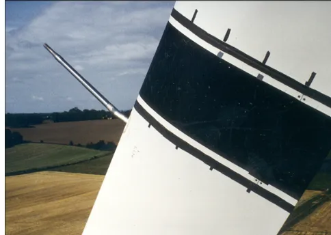
In 1989, a pitot tube was mounted on a 95 kW Tellus tur-bine; see Fig. 1. The turbine was a fixed-pitch, constant-speed, stall-regulated turbine with rather stiff blades; i.e. the angle of attack, measured by the pitot tube, is highly corre-lated with the axial wind speed at the pitot tube.
A subset of the Tellus measurement dataset has been procured for this study. In Fig. 2, the 30 s mean power-production observations are plotted as a function of the an-gle of attack (a) and met-mast wind speed (b). The met mast is located 2.5 diameters from the turbine, and observations
Figure 1.Five-hole pitot tube mounted on the blade of a 95 kW Tellus turbine at Risø in 1995.
where the met mast is in the wake are excluded from Fig. 2b. It is seen that the power production correlates much more highly with the angle of attack than with the met-mast wind speed, especially below stall.
The quality of a power curve depends on the number of data points and the scatter of these points; furthermore, all regions of the curve must contain enough data points. The number of data points can be increased by extending the mea-surement period, but it can also be increased by reducing the averaging time. In Fig. 3 the averaging time of the pitot-tube-based plot is reduced to the time of one revolution (∼1.25 s); i.e. around 24 times more data points are obtained from the same measurement period, and the scatter level is still lower than the met-mast-based 30 s mean observations in the region below stall.
This means that the assessment time can be significantly reduced, as many more data points with less scatter are ob-tained and in addition rarely occurring wind speeds are more likely to occur for a 1.25 s than for a 30 s averaging period.
Today, 28 years later, standard wind turbines are pitch reg-ulated and operated with variable speed and have a 5–10 times larger rotor and very flexible blades. In this paper we will therefore investigate if a similar speed-up in power and flap load assessment time is achievable by using pitot-tube measurements as an inflow reference on modern megawatt wind turbines such that a power curve and load validation can be conducted from a few days of measurements.
The study is based on aeroelastic simulations using the code HAWC2 (Larsen and Hansen, 2007) and measurements on a Siemens 3.6 MW wind turbine.
2 Method
Figure 2.The 30 s mean electrical power of the Tellus turbine correlates much more highly with the angle of attack(a)than the met-mast wind speed(b).
Figure 3.Despite the much lower average time – one revolution (∼1.25 s) instead of 30 s – the average scatter level of the pitot-tube-based observations(a)is still lower than the level of the met-mast-based observations in the region below stall(b).
error measure that is used to evaluate the quality of power and flap load curves.
2.1 Deriving the wind speed from the angle of attack on the Tellus turbine
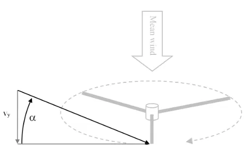
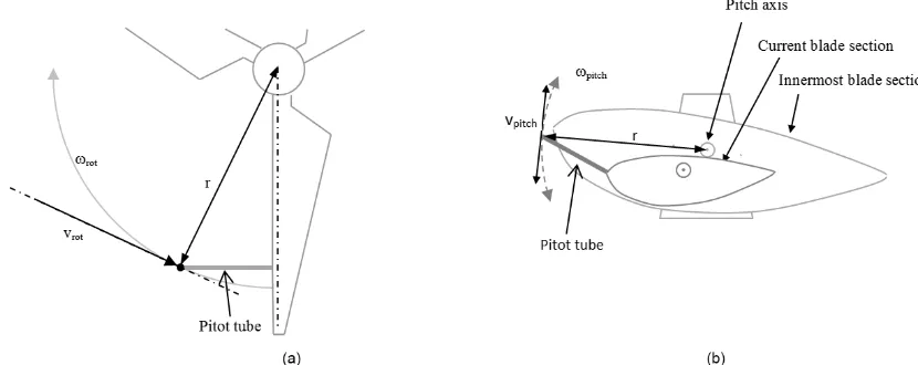
For the Tellus turbine which has a fixed pitch, constant rotor speed and rather stiff blades, the axial wind speed at the pitot tube,vy, is a function of the rotor speed,vrot, and the angle
of attack,α(see Fig. 4):
vy=tan (α)vrot→α∝atan vy. (1)
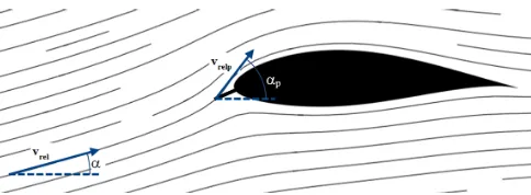
The inflow angle measured by the pitot tube, αp, obviously
depends on the angle of the pitot tube but also on the posi-tion due to increased upwash near the airfoil; see Figure 5. In general the relation between the angle of attack and the flow angle at a point near the airfoil, Fα, is nonlinear but
mono-tonically increasing in the region of interest if the effects of dynamic stall are neglected.
The Tellus turbine has 5◦tilt (angle between shaft and hor-izontal); i.e. αp is increased when the blade moves up and
Figure 4.In the simple case, the axial wind speed,vy, is a mono-tonic function ofα.
vice versa, so thatupbecomes
vy=cos (θtilt) tan Fα αp+θpitot−θtiltsin θrotorpositionvrot. (2)
when averaging over one or more revolutions.
2.2 Deriving the wind speed from pitot-tube measurements of modern wind turbines
For modern wind turbines with variable pitch and rotor speed,αpcannot be used directly as a measure of the axial
wind speed. In this case the following procedure is used:
– determine the angle of attack and relative velocity from the flow angle and velocity measured by the pitot tube
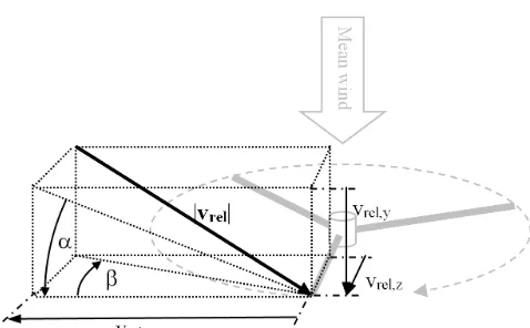
– map the angle of attack, relative velocity and pitot-tube side-slip angle from spherical coordinates to a 3-D Cartesian flow vector
– determine and subtract the velocity due to the move-ment of the pitot tube
– map the wind speed vector onto global coordinates and extract the horizontal component.
2.2.1 Estimating the angle of attack
At the pitot-tube tip, i.e. near the airfoil, the flow angle,αp,
and the relative speed,|vrelp|, are different due to local
circu-lation around the blade section and deceleration of the flow; see Fig. 5. The first step is therefore to find the angle of at-tack,α, and the relative speed,|vrel|.
For the simulations, this step is not necessary, as HAWC2 directly computes α and|vrel| based on the blade element
momentum (BEM) model.
For the measurements, 2-D computational fluid dynamics (CFD) simulations have been used to compute the velocity, vrelp, for different angles of attack. From these velocities two
functions are generated. The first function,Fα, mapsαptoα
(see Fig. 6a), while the second,Fvrel, gives the flow speed at
the pitot tube,|vrelp|, relative to the flow speed some distance
upstream,|vrel|:
|vrel| = vrelp
Fvrel(α)
; (3)
see Fig. 6b.
and, now,vrel vrel,x vrel,y vrel,z can be derived:
vrel,x= − s
|vrel|2
1+(tanα)2+(tanβ)2 , for |β| ≤90
◦
s
|vrel|2
1+(tanα)2+(tanβ)2 , for
|β|>90◦
, (7)
vrel,y= − v u u u t
|vrel|2
1 tanα
2
+1+tanβ tanα
2 , for α >0
0 , forα=0
v u u u t
|vrel|2
1 tanα
2
+1+tanβ tanα
2 , for α <0 , (8)
vrel,z= v u u u t
|vrel|2
1 tanβ
2 +tanα
tanβ 2
+1
, forβ >0
0 , forβ=0
− v u u u t
|vrel|2
1 tanβ
2 +tanα
tanβ 2
+1
, forβ <0 . (9)
2.2.3 Estimate and subtract the movement of the pitot tube
The pitot-tube movement derives from three factors: the rotor speed, pitch motions and the speed due to blade deflection.
The rotor speed contributes with a tangential speed,vrot,
which is the product of the rotor speed,ωrot, and the radius
of the pitot-tube tip; see Fig. 8a. Note that the radius changes during pitch motion.
Similarly, pitch motions also result in a velocity,vpitch,
tan-gential to the pitch axis; see Fig. 8b.
As the speed due to blade deflection cannot be extracted from the current measurement database, this contribution is not included in the present study. The error introduced by this simplification is, however, analysed in Sect. 4.3.
co-Figure 6.(a)Angle of attack,α, as a function of flow angle measured by pitot tube,αp.(b)Relative speed at position of pitot tube as a function of the angle of attack.
Figure 7.Relation between (α,β,|vrel|) and [vrel,x,vrel,y,vrel,z]T.
ordinate system (indexed B) and subtracted.
vB=VrelB−vBrot−vBpitch (10)
2.2.4 Map to global coordinates
Finally the flow velocity is mapped to a global coordinate system using rotation from pitch, coning (downwind angle of blades relative to a line perpendicular to the shaft) , rotor position and tilt, and the horizontal wind speed component parallel to the main shaft,vy, is extracted.
2.3 Power of variable-speed wind turbines
Wind turbines convert aerodynamic power to electrical power, but some energy is “stored” as angular momentum in the rotor. When dealing with small timescales on mod-ern variable-speed wind turbines, the fraction of the aerody-namic power used to accelerate or decelerate the rotor may be significant. To include this energy buffer, the power ob-servations used in this study are compensated for rotor speed
variations when the power is below rated power by
Power=Powerelectric+ 1 2I
ω2rot,t1−ωrot,t22
t2−t1 , (11)
whereIis the inertia of the rotor,ωrotis the rotational speed,
andt1 andt2 are the start and end time of the observation period, e.g. one revolution.
2.4 Performance curves
First the observations are binned based on their wind speed values. In this study bins of 0.5 m s−1 ranging from 3 to 18 m s−1are used. For each bin the mean wind speed is calcu-lated as well as the mean power/flap load, and then the power and flap load performance curves are generated by linear in-terpolation between these mean values.
2.5 Error measure
The accuracy of the pitot-based power and load curves can-not be evaluated in its present form as the curves cancan-not be compared to reference curves of existing methods that are based on free-flow wind speed. We will therefore focus on variability between periods or cases instead of accuracy.
If the curves obtained in similar conditions are equivalent, then it will be possible to make a small adjustment on the rotor, e.g. changing the tip shape or vortex generator con-figuration, and to determine whether the change affects the power production or load levels.
For this purpose the variation in terms of the mean stan-dard deviation will be used.
Figure 8.Rotor rotation(a)and pitch motion(b)moves the pitot tube and contributes to the flow speed measured by the pitot tube.
load is used as an error measure:
Variation=
1 M
P j=1..M
r 1 N
P i=1..N
PCi wspj
−PC wspj 2
max(PC) . (12)
In the parameter study referred to in Sect. 5.2, the effects of different inflow conditions are investigated by changing an inflow parameter, e.g. the turbulence intensity, and com-paring the resulting power and load curves to a reference curve. In this case the error measure is modified, such that the curves are compared to the reference curve:
Variation=
1 M
P j=1..M
r
PC wspj−PCref
wspj2
max(PC) . (13)
3 Numerical study
In this section, simulation results are used to investigate the optimal averaging time, the uncertainties introduced by blade deflection and torsion and the optimal radial position of the blade-mounted flow sensor. Finally, a numerically based es-timation of the achievable assessment time reduction is pre-sented.
The simulations are performed using HAWC2, which is a nonlinear aeroelastic code intended for computing wind tur-bine response in the time domain (Aagaard Madsen et al., 2010b, 2012; Kim et al., 2013; Larsen et al., 2015).
The turbine model used for the simulations is based on the structural and aerodynamic configuration of the Siemens 3.6 MW turbine, which was tested at Høvsøre in 2009 during the DANAERO project (Aagaard Madsen et al., 2010a), i.e. a model of the turbine in the full-scale measurement study in Sect. 5.
3.1 Simulation overview
For the analysis, different simulation sets have been created; see Table 1. All simulation sets contain 30 min of simulation for each wind speed ranging from 3 to 18 m s−1in 0.5 m s−1 steps, i.e. 15.5 h of simulation per set.
3.2 Averaging time
For IEC standard power curves, 10 min mean values are re-quired (IEC 61400-12-1, 2005), but in this study shorter av-erage times are also used.
Reducing the averaging time results in more observations with more variation. If the correlation between wind speed and power/load is high, this variation adds usable informa-tion, and the uncertainty of the power/load curve decreases. If, on the other hand, the correlation is low, the variation mainly results in more scatter, and nothing is achieved.
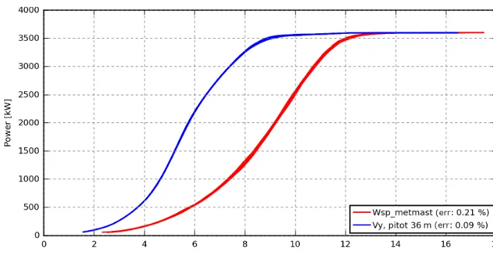
To investigate the optimal averaging time, the mean stan-dard deviation of 16 power/load curves has been calculated for different averaging times, ranging from 1 to 600 s. The 16 curves are based on the 16 simulation sets in SIM1; see Table 1. Figure 9 shows an example of the 16 power curves generated from 15 s mean values. The mean variation in the met-mast-based power curves is 0.21 % of rated power, while it is 0.09 % for the pitot-based curves.
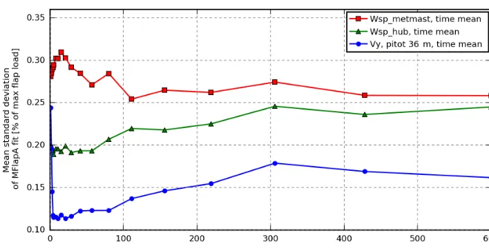
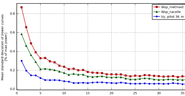
The variation is plotted in Fig. 10 as a function of aver-aging time for power curves based on met-mast wind speeds, free-flow wind speeds at the hub centre and wind speeds from a pitot tube at 36 m.
Table 1.Overview of simulations and parameters.
Id No. No. Turb. intensity Shear Yaw misalign. Air density
sets seeds (%) (power coefficient) (deg) (kg m−3)
SIM1 16 16 Meas.* Meas.* 0 1.225
Ref 5 5 7.5 0.1 0 1.225
Shear 6 1 7.5 0.01, 0.2, 0.3, 0.4, 0.5, 0.6 0 1.225
Ti 7 1 2.5, 5,. . . , 20 0.1 0 1.225
Yaw 5 1 7.5 0.1 2.5, 5, 7.5, 10 1.225
Dens 4 1 7.5 0.1 0 1.175, 1.2, 1.25, 1.275
* For each wind speed, the mean turbulence intensity and power shear coefficient are extracted from the measurements.
Figure 9.Example of simulated power curve variation based on 15 s mean values. The variation in the 16 met-mast-based curves is twice the variation in the 16 pitot-based curves.
variation is expected to be introduced by tower deflections and the disturbed-to-free-flow transfer function.
The variation in the hub centre and pitot-based curves decreases with shorter averaging times, while the variation in the met-mast-based curves is almost constant due to the lower correlation. In simulations, where the inflow is station-ary, the met-mast and hub-centre variations will coincide for longer average times, but in practice long average times are not appropriate due to the non-stationary nature of real in-flow.
For average times below one revolution, the variation in the pitot-based curves increases significantly as shear- and turbulence-induced local wind speed variations within the ro-tor are not averaged out.
Figure 11 shows similar results for the flap moment curves.
3.3 Uncertainty due to blade and tower deflection
During operation, the structure of a modern wind turbine moves and the blades deflect and twist considerably. The mo-tion contributes to the movement of the blade-mounted flow
sensor and thereby the measured flow velocity. When calcu-lating the wind speed, the velocity of the sensor should be subtracted from the measured flow velocity, but in this case the velocity deriving from blade deflection is unknown and consequently cannot be subtracted. In addition, blade deflec-tion changes the orientadeflec-tion of the sensor such that the mea-sured flow speed cannot be mapped onto the true global co-ordinates, as the true orientation is unknown.
The error that these effects introduce to the estimated wind speed has been investigated using numerical simulations. From the first simulation set in SIM1 (see Table 1), pitot-tube data, i.e.α,β,vrel, were output at 11 different radial
positions on the blade ranging from the root to the tip. Based on the pitot-tube data, the estimated global wind speed in-cluding velocity due to blade deflection was calculated and compared to simulated “real” wind speed.
Figure 10.Mean standard deviation of simulated power curves based on met-mast wind speed, free wind speed at the hub centre and wind speed from pitot tube at 36 m. The variation is shown for observation average times ranging from 1 to 600 s.
Figure 11.Mean standard deviation of simulated blade flap moment based on met-mast wind speed, free wind speed at the hub centre and wind speed from pitot tube at 36 m. The variation is shown for observation average times ranging from 1 to 600 s.
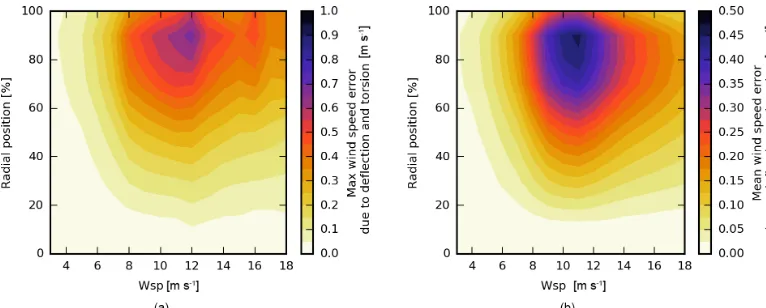
At 70 %, i.e. close to the position of the pitot tube in the measurements, the maximum error is around 2 m s−1, while the mean error is up to 0.5 m s−1. This means that the in-stantaneous wind speed estimated from the pitot-tube data is inappropriate for power and load assessment. In this study however, we use the mean of one revolution as the lowest observation average time, and during one revolution the ve-locity caused by small-scale turbulence-induced deflections as well as 1P (one-per-revolution) periodic deflections, e.g. due to shear, is almost averaged out, as seen in Fig. 13, where the errors of the one-revolution means are shown.
The major part of the remaining error is caused by a static deflection of the blade, which changes the orientation of the sensor. This error is related to the thrust on the rotor and peaks around rated wind speed. For a flow sensor mounted at
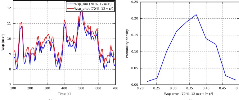
70 % in 12 m s−1, Fig. 14a reveals an almost constant offset between the simulated “real” wind speed and the wind speed estimated from the virtual pitot-tube data, which is confirmed by the error distribution plot in Fig. 14b.
The constant part of the error will shift thex axis of the power and load assessment curves in a nonlinear way, but it will not introduce additional variation when comparing power and load curves of different periods, and it can there-fore be neglected in this study.
Figure 12.Maximum(a)and mean(b)simulated wind speed error in the axial direction due to deflection and torsion.
Figure 13.Maximum(a)and mean(b)simulated error of the wind speed (one-revolution mean) in the axial direction due to deflection and torsion.
3.4 Optimal radial position of blade-mounted flow sensors
A flow sensor mounted near the root will only sweep a small area of the rotor plane, while a flow sensor mounted near the tip will suffer from large deflections, torsion and tip loss effects. From the 16 simulation sets in SIM 1 (see Table 1), power curves are generated based on one-revolution mean values from pitot tubes at different radial positions. The mean standard deviation of these curves is seen in Fig. 16a as a function of radial position. It is seen that a pitot tube at 70 % results in the lowest variation. This means that the position of the pitot tube in the measurements is close to optimal. Using the mean of the wind speeds measured by the pitot tubes at 20, 50 and 80 % gives power curves with only slightly lower variation.
For the flap moment curves, the optimal sensor position is around 50 %; Fig. 16b. In this case a slightly lower variation is also seen when using the mean wind speed measured by three pitot tubes.
3.5 Potential assessment time reduction
In this section we want to quantify the potential assessment time reduction that can be achieved – based on simulations. Due to the higher correlation between the blade-mounted flow sensor wind speed and the power/flap loads, it is ex-pected that fewer observations are required to reach a cer-tain variation level. To quantify the reduction, the variance in power curves generated from 1 to 36 h of one-revolution mean observations is calculated; see Fig. 17. The observa-tions used for the power curves are uniformly distributed; i.e. each of the 1 h power curves is based on approximately 2 min of each simulated wind speed from 3 to 18 m s−1.
It is seen that it requires 36 h of observations based on met-mast wind speed and 15 h of observations based on nacelle wind speed to reach the error level obtained from 4 h of ob-servations using the pitot tube at 36 m. In general the speed-up achieved by using pitot-tube-based observations instead of met-mast-based observations is around 7.
Figure 14.(a)Time series of simulated “real” wind speed and simulated wind speed estimated from pitot-tube data.(b)Distribution of the simulated error.
Figure 15.Maximum(a)and mean(b)simulated error of the wind speed (one-revolution mean neglecting the average offset) in the axial direction due to deflection and torsion.
all wind speeds are observed in the same hour – and therefore a similar speed-up cannot be expected in reality.
4 Full-scale measurement study
In this section, we investigate whether the wind speeds that can be derived from the pitot tube are also highly correlated with the power and flap loads in practice. The results are based on measurements of a full-scale modern wind turbine with a blade-mounted five-hole pitot tube. Furthermore, we address whether more power and flap moment curves with less variation can be obtained by using pitot-tube wind speed instead of met-mast-recorded wind speeds.
4.1 Turbine and site
The measurement data of the 3.6 MW Siemens turbine stems from the DANAERO project 2007–2009 (Aagaard Madsen et al., 2010a). The turbine was located at the Høvsøre test site for large wind turbines in Denmark and equipped with a
five-hole CPSPY5 Aeroprobe pitot tube at the 36 m radius of one of its 53.5 m blades.
The turbine is located in the middle of a row of five large turbines, and around 3 months of measurement data are avail-able on the turbine and the nearby met masts; see Fig. 18.
4.2 Effects of shear and turbulence intensity, yaw error, and air density on power and flap load curves
Figure 16.Mean relative standard deviation of simulated power(a)and flap load(b)fits based on wind speed from pitot tubes at different radial positions. The pitot tube at 36 m, which corresponds to the position of the pitot tube in the measurements, is close to optimal for the power curves, while the mean of three pitot tubes at 20, 50 and 80 % provides slightly less variation.
Figure 17.Mean relative standard deviation of simulated power curves based on uniformly distributed observations. Using the pitot-tube instead of the met-mast wind speed as the basis for the power curves, the same error level can be achieved approximately 7 times faster.
shear levels, yaw errors and air densities, without changing the power and load curves too much.
These limits have been found by comparing the reference simulation sets with the sets where different turbulence inten-sities, shear levels, yaw misalignment angles and air densities have been simulated (see Table 1) in terms of the mean abso-lute difference between the power and load curves in percent of maximum power and load; cf. Eq. (13).
The power and load curves are highly dependent on the turbulence intensity, which must be in the range of 3–12 % to keep the mean absolute difference below 0.5 %.
For every 10 min of measurements, a shear profile coeffi-cient is calculated by fitting a power shear profile to the one hour mean wind speed measured by the main met mast at 10, 40, 60, 80, 100 and 116.5 m height. Most observations have a power shear coefficient below 0.3, which has been found to keep the mean absolute difference below 0.5 %, and the rest is discarded.
Figure 18.Overview of the Høvsøre test site for large turbines in Denmark. The Siemens turbine is located in the middle of a row of five turbines.
The aerodynamic power and loads are proportional to the density of air for constant power and load coefficient, and therefore the normalization
Powernormalised=Power10 min
ρ0
ρ10 min
(14)
must be used for power curves of stall-regulated turbines (IEC 61400-12-1, 2005). Pitch-regulated turbines on the other hand reduce the power coefficient at high wind speeds to maintain rated power. Therefore, another normalization, which normalizes the free-flow wind speed, is used for pitch-regulated turbines. However, in this context we are using the pitot wind speed, and therefore the above normalization is applied up to rated wind speed from where it is faded out. When using this normalization, no limits are required on the air density to keep the mean absolute difference below 0.5 %.
4.3 Selecting measurement observations
A huge effort has been invested in selecting a proper set of observations from the measurement database as well as in correcting or discarding error-prone sensor observations.
The measurement database consists of 1600 h of measure-ment, but only a few hundred hours are usable for this analy-sis; see the summary of the selection process in Table 2. The wake filter discards more met-mast observations than pitot observations as the met mast, i.e. Mast 3 in Fig. 18, is in the wake of the turbines in easterly wind directions, but many of these cases are discarded anyway as the turbulence intensity or shear coefficient is outside the accepted range. The final
filter that rejects datasets containing corrupted or suspicious pitot observations reduces the amount of observations for the pitot-based analysis far below the amount of observations us-able for met-mast-based analysis.
4.4 Pitot inclusion criteria
The current pitot-tube system is very sensitive to rain, es-pecially the P1–P6 sensor, which records the pressure dif-ference between the centre hole and the static ring. Figure 19 shows the typical behaviour of the P1–P6 sensor, before, dur-ing and after rainfall. Before the rain starts, the P1–P6 sen-sor output is independent of rotor position (Fig. 19a), and the first droplets are clearly seen as spikes and sinusoidal patterns; Fig. 19b and c. During the rainfall, water gets in-side the tubes and the output becomes continuous sinusoidal; Fig. 19d. During the next couple of hours different more or less abnormal patterns are recorded until the water suddenly disappears and a signal independent of rotor position is re-stored; Fig. 19e–h. These effects of rainfall have not been detected in the measurements from a previous experiment (Aagaard Madsen et al., 2003), where a Rosemount M858 pitot tube (Schmidt Paulsen, 1990) was used.
Table 2.Measurement selection filters.
Filter Pitot observations Met mast Comments (h) observations (h)
Total 1599 1599
Normal operation 926 926 Filter on turbine status signal, rpm>2 and power>100 kW
Variable rpm 858 858 In the discarded period the turbine was operated with constant rotor speed
No wake 629 528 Avoid wake situations
Turbulence intensity 537 414 Discard observations with turbulence intensity outside the range 0.03–0.12
Shear 481 414 Discard observations with power shear coefficient out-side the range 0–0.3
Pitot ok 242 407 Discard observations where pitot-tube data are uncer-tain; see Sect. 5.4
Figure 19.The background plot shows the cumulated rain from 27 to 28 April 2009. Approximately 2.5 mm rain fell between 16:00 and 17:30 LT (UTC+2). The coloured points indicate the temporal position of the corresponding graphs on the timeline. These graphs show the P1–P6 sensor (pressure difference between centre hole and static ring) as a function of rotor position (0◦: blade down; 180◦: blade up) over a period of 10 min.(a)Before the rain, P1–P6 is almost constant. Panels(b)and(c): first droplets cause spikes and sinusoidal patterns.(c)
Water in the tubes is now constantly causing sinusoidal output.(e)Sinusoidal output when the blade is in the upper part only.(f–h)Transition from disturbed to normal recording.
a rough filter that discards observations made between 1 h prior to rainfall and 12 h after rainfall is applied in this study. Over an interval of approximately 1 month in the middle of the measurement period, spikes are often seen in the output of the P1–P6 sensor; see Fig. 20a. Often the spikes occur at a fixed rotor position for some time, as seen in Fig. 20b, but the position moves from time to time. In many cases the duration
of the spike is only a few degrees as in Fig. 20b, while in other cases the sensor output level seems to be increased for half a revolution.
Figure 20.Output of the P1–P6 sensor (pressure difference between centre hole and static ring) as a function of time(a)and rotor position
(b). Spikes are clearly seen around 260◦.
The sensors P2–P3 and P4–P5, which record the inflow and side-slip angle, respectively, also have periods with ab-normal sinusoidal patterns. These periods are more distinct but not related to rainfall, and in this study they are iden-tified based on their 1P (one-per-revolution) Fourier coeffi-cients values.
4.5 Pitot wind speed correlation with power and flap load
Figure 21 shows the power (a and c) and flap load (b and d) observations measured on the 9 and 10 May as a function of pitot and met-mast wind speeds. In (c) and (d) the met-mast observations represent 600 s mean values, while all other ob-servations are 120 s mean values. The pitot-based observa-tions have less scatter than the 120 s met-mast observaobserva-tions (a and b), while they are comparable to the 600 s met-mast observations which comprise far fewer observations (c and d).
These results are similar to the results from the Tellus ex-periment (see Figs. 2 and 3) and indicate that it is possible to reduce the scatter of the power and load observations or in-crease the number of observations by using pitot-tube instead of met-mast recordings – also on modern wind turbines.
In Fig. 21, the pitot observations are based on 120 s mean values. The simulation results in Fig. 10, however, indicate that the best results are obtained from averaging times be-tween one revolution and 30 s. Figure 22a shows the power observations from a 10 min period based on 600 s, 120 s and one-revolution mean values. The five 120 s mean values pro-vide information about the slope of the curve in contrast to the single 600 s observation, while the one-revolution mean observations provide information about an even wider range
of wind speeds. The scatter of the one-revolution mean obser-vations, however, is remarkable. The scatter is mainly caused by a pitch motion procedure, which changes the pitch angle by 1◦every minute to exercise the pitch bearings. These pitch steps result in two levels and increased scatter in both hori-zontal and vertical directions as both power and pitot wind speeds are affected (Hansen et al., 2005). In Fig. 22b, the one-revolution mean observations are coloured according to the current pitch state, which is seen to split the observations in two less scattered groups. Unfortunately this means that the averaging time must be at least 120 s to average out the scatter caused by the pitch motion procedure.
In Fig. 21, the pitot-based power and flap load observa-tions over a 2-day period were located on a relatively thin line. Plotting all observations, however, results in a thick belt instead of a thin line; see Figs. 23 and 24. Colouring the ob-servations according to the time of recording reveals that in many periods the observations are describing a relatively thin line, but the line shifts from time to time.
Figure 21.Measured power(a, c)and flap load(b, d)observations as a function of pitot and met-mast wind speed. In(a, b)all observations are 120 s mean values, while the met-mast observations in(c, d)are 600 s mean values. Using pitot instead of met-mast wind speed, the amount of scatter can be reduced(a, b)or more observations can be obtained(c, d).
4.6 Number and variation in performance curves
In Sect. 4, the comparison of uniformly distributed simula-tion observasimula-tions showed that the number of hours required to obtain power curves with a variation level below a cer-tain threshold can be reduced around 7 times by using pitot-based instead of met-mast-pitot-based wind speeds. This result was based on one-revolution mean values, which in Sect. 4.2 were found to give the lowest variation. However, this is not feasible for the measurements, due to the scatter introduced by the pitch motion procedure.
In practice it is not possible to obtain a full power curve, e.g. every 4 h, as both low- and high-wind situations must oc-cur, and from the current measurement database only a few power curves can be obtained. The exact number of curves depends on the wind speed range and resolution of interest. In the following analysis, the range from 4 to 13 m s−1
(met-mast wind speed) is divided into bins of 0.5 m s−1. Observa-tions are then collected for the first power curve until all bins contain at least three observations, then for the next power curve, etc.
Figure 25 shows the resulting power curves and the under-lying observations. In this case the pitot-based approach pro-vides three curves with 1.1 % variation (percent of maximum power), while four curves with slightly higher variation are obtained from the met-mast-based observations. This means that from the current measurement database, an assessment time reduction cannot be achieved by using pitot-tube wind speed instead of met-mast wind speed.
in-Figure 22.(a)Reducing the averaging time increases the number of observations and gives information about a wider wind speed range. Averaging times below 120 s, however, results in a remarkable amount of scatter, which is mainly caused by a pitch motion procedure.
(b) The one-revolution mean values are coloured according to the pitch state; i.e. black points are observations where the pitch angle is increased by 0.5◦and cyan points are observations where the pitch angle is decreased by 0.5◦. The pitch state splits the observations into two less scattered groups.
Figure 23.Measured power observations from the entire database. In many periods, the pitot observations describe a relatively thin line, but the line shifts from period to period.
dication of the optimal potential has been achieved by re-laxing the constraints, i.e. suppressing the pitot ok filter and using one-revolution mean values. In this optimal case, the pitot-based approach results in 20 power curves, and the 19 June produces four power curves in a single day, i.e. the same number as obtained from the whole period using the met-mast-based approach. Note, however, that the variation in these curves may be significant due to shorter averaging times and the line shifting seen in Figs. 23 and 24.
5 Conclusions
In the numerical part of this paper it is shown that the wind speed derived from a blade-mounted flow sensor of a modern pitch-regulated, variable-speed wind turbine correlates more highly with the power and flap loads than the wind speed measured 2.5 diameters upstream. The correlation is also higher than the wind speed that can be obtained from a fixed-point instrument, e.g. a nacelle-mounted cup anemometer.
ob-Figure 24.Measured flap load observations from the entire database. In many periods, the pitot observations describe a relatively thin line, but the line shifts from period to period.
Figure 25.Only two or three full-range power curves can be obtained from the current measurement database.
servation average times, in the range of 5–90 s, reduce the variation in the curves.
Deflection and torsion of the blades introduce an error into the wind speed derived from a blade-mounted flow sensor. When averaging over one or more revolutions, the error is significantly reduced and the major part of the remaining er-ror is a constant offset, which can be ignored when power and flap load curves of different periods are compared. For the current turbine the radial flow sensor position that results in the lowest variation in power curves was found to be 70 %, while a sensor in 50 % is optimal for flap load curves.
Finally, the analysis showed that the length of the assess-ment period, which is required to achieve a certain power or flap load curve variation can be reduced around 7 times by
using uniformly distributed wind speed observations from a blade-mounted flow sensor instead of a met mast.
The measurement part of the paper concludes that the cur-rent pitot-tube system is highly sensitive to rain, and a proper algorithm must be applied to discard error-prone observa-tions.
not be possible to put a met mast. It can be used to inves-tigate aerodynamic modifications or detect performance is-sues, e.g. due to leading-edge roughness, by comparing the relative pitot-based power and load curve between different periods or turbines. In addition it follows the yaw direction; i.e. it is never in the wake of the current turbine in contrast to a traditional met mast. Moreover additional information about the angle of attack, wind speed variations within the rotor plane (e.g. shear, veer, height-dependent turbulence in-tensity) and wake effects can be extracted. This information can be used as input for the control of individual pitch or ac-tive trailing-edge flap to optimize power and/or reduce loads or noise (Larsen et al., 2005; Barlas et al., 2012; Kragh and Hansen, 2012; Kragh et al., 2012; Aagaard Madsen, 2014).
The measured wind speeds are, however, affected by the wind turbine induction. This means that it cannot be used for IEC standard power curves, and changing the induction, e.g. by another control strategy, yaw misalignment or by the pitch step procedure seen in the present study, will shift the resulting wind speed. Another problem is that the induced wind speeds increase up to rated power; i.e. in this region the flow-sensor-based power curve has a higher slope, which for the present turbine was found to be almost vertical around rated rotor speed, such that small wind speed uncertainties result in large power variations.
a blade-mounted flow sensor is highly correlated with the power and flap loads, especially during shorter periods, but the potential assessment time speed-up that was obtainable in the simulation could not be confirmed from the current measurements.
Blade-mounted flow sensors are, however, able to provide additional valuable information about the inflow variations within the rotor plane, but a robust instrument and measure-ment system is required to extract reliable wind speed mea-surements.
Appendix A: List of symbols
α Angle of attack
αp Inflow angle measured by pitot tube
β Side-slip angle; see Fig. 7
Fα Function mappingαpontoα
Fvrel Function mapping vrelponto vrel
I Inertia of rotor
ωpitch Angular pitch speed of blade with pitot tube
ωrot Angular rotational speed
vrel=vrel,x vrel,y vrel,z Flow velocity at pitot tube relative to the sensor adjusted for reduced
flow velocity and deflection near the airfoil due to bound circulation vrelp=vrelp,x vrelp,y vrelp,z Relative flow velocity measured by the pitot tube including effects of
bound circulation
vrot Velocity caused by blade rotation
vpitch Velocity of pitot tube due to pitch motion
v=vx vy vz Wind velocity at position of pitot tube including induction effects (vyis
horizontal in direction of main shaft)
θtilt Tilt angle
θrotorposition Azimuthal angle of blade with pitot tube
θpitot Angle of pitot tube relative to the centre line of the blade
θpitch Pitch angle of blade with pitot tube
vrel Relative flow speed at pitot tube, compensated reduced flow velocity
References
Aagaard Madsen, H.: Aerodynamics and Structural Dynamics of a Horizontal Axis WindTurbine – Raw Data Overview, Technical Report Risø-M-2902, Risø National Laboratory, Roskilde, Den-mark., 1991.
Aagaard Madsen, H.: Correlation of amplitude modulation to inflow characteristics, Proc. 43rd Int. Congr. Noise Con-trol Eng., available at: http://www.acoustics.asn.au/conference_ proceedings/INTERNOISE2014/papers/p171.pdf (last access: 13 November 2017), 2014.
Aagaard Madsen, H., Thomsen, K., and Petersen, S. M.: Wind Tur-bine Wake Data from Inflow Measurements using a Five hole Pitot Tube on a NM80 Wind Turbine Rotor in the Tjæreborg Wind Farm, Technical Report Risø-I-2108, Risø National Lab-oratory, Roskilde, Denmark, 2003.
Aagaard Madsen, H., Bak, C., Schmidt Paulsen, U., Gaunaa, M., Fuglsang, P., Romblad, J., Olesen, N. A., Enevoldsen, P., Laursen, J., and Jensen, L.: The DAN-AERO MW Experiments: Final report, Danmarks Tekniske Universitet, Risø Nationallab-oratoriet for Bæredygtig Energi, available at: orbit.dtu.dk (last access: 13 November 2017), 2010a.
Aagaard Madsen, H., Bak, C., Døssing, M., Mikkelsen, R. F., and Øye, S.: Validation and modification of the Blade Element Momentum theory based on comparisons with actuator disc simulations, Wind Energy, 13, 373–389, https://doi.org/10.1002/we.359, 2010b.
Aagaard Madsen, H., Riziotis, V., Zahle, F., Hansen, M. O. L., Snel, H., Grasso, F., Larsen, T. J., Politis, E., and Rasmussen, F.: Blade element momentum modeling of inflow with shear in comparison with advanced model results, Wind Energy, 15, 63– 81, https://doi.org/10.1002/we.493, 2012.
Antoniou, I., Wagner, R., Markkilde Petersen, S., Schmidt Paulsen, U., Madsen Aagaard, H., Ejsing Jørgensen, H., Thomsen, K., Enevoldsen, P., and Thesbjerg, L.: Influence of wind characteris-tics on turbine performance, in: Conference proceedings, Euro-pean Wind Energy Association (EWEA), 2007.
Barlas, T. K., van der Veen, G. J., and van Kuik, G. A. M.: Model predictive control for wind turbines with distributed active flaps: incorporating inflow signals and actuator constraints, Wind En-ergy, 15, 757–771, https://doi.org/10.1002/we.503, 2012. Eggers A. J., J., Digumarthi, R., and Chaney, K.: Wind Shear and
Turbulence Effects on Rotor Fatigue and Loads Control, 75944, 225–234, https://doi.org/10.1115/WIND2003-863, 2003.
dtu.dk (last access: 13 November 2017), 2005.
IEC 61400-12-1: Power performance measurements of electricity producing wind turbines, International Electrotechnical Com-mission, Geneva, Switzerland, available at: www.iec.ch, 2005. Kim, T., Hansen, A. M., and Branner, K.: Development of an
anisotropic beam finite element for composite wind turbine blades in multibody system, Renew. Energ., 59, 172–183, https://doi.org/10.1016/j.renene.2013.03.033, 2013.
Kragh, K. and Hansen, M.: Individual Pitch Control Based on Local and Upstream Inflow Measurements, in: 50th AIAA Aerospace Sciences Meeting including the New Horizons Forum and Aerospace Exposition, Reston, Virigina, American Institute of Aeronautics and Astronautics, https://doi.org/10.2514/6.2012-1021, 2012.
Kragh, K. A., Henriksen, L. C., and Hansen, M. H.: On the Po-tential of Pitch Control for Increased Power Capture and Load Alleviation, Presented at The Science of Making Torque from Wind 2012, 9–11 October 2012, Oldenburg, Germany, available at: orbit.dtu.dk (last access: 13 November 2017), 2012. Larsen, T. J. and Hansen, A. M.: How 2 HAWC2, the user’s manual,
Technical Report, Risø National Laboratory, Roskilde, Denmark, available at: orbit.dtu.dk (last access: 13 November 2017), 2007. Larsen, T. J., Aagaard Madsen, H., and Thomsen, K.: Ac-tive load reduction using individual pitch, based on lo-cal blade flow measurements, Wind Energy, 8, 67–80, https://doi.org/10.1002/we.141, 2005.
Larsen, T. J., Larsen, G., Aagaard Madsen, H., and Petersen, S. M.: Wake effects above rated wind speed . An overlooked contributor to high loads in wind farms, in: Scientific Proceedings, EWEA Annual Conference and Exhibition, Paris, France, 95–99, Euro-pean Wind Energy Association (EWEA), 2015.
Pedersen, M. M., Larsen, T. J., Larsen, G. C., and Mad-sen, H. A.: Turbulent wind field characterization and re-generation based on pitot tube measurements mounted on a wind turbine, in 33rd Wind Energy Symposium, Kissimmee, Florida, American Institute of Aeronautics and Astronautics, https://doi.org/10.2514/6.2015-1467, 2015.
Petersen, J. T. and Aagaard Madsen, H.: Risø-R-993(EN): Local Inflow and Dynamics – Measured and Simulated on a Rotating Wind Turbine Blade, Risø National Laboratory, Roskilde, Den-mark, 1997.
St. Martin, C. M., Lundquist, J. K., Clifton, A., Poulos, G. S., and Schreck, S. J.: Wind turbine power production and annual en-ergy production depend on atmospheric stability and turbulence, Wind Energ. Sci., 1, 221–236, https://doi.org/10.5194/wes-1-221-2016, 2016.