Comparison and application of wind retrieval algorithms for small unmanned aerial systems

(1)

Geosci. Instrum. Method. Data Syst., 2, 177–187, 2013 www.geosci-instrum-method-data-syst.net/2/177/2013/ doi:10.5194/gi-2-177-2013

EGU Journal Logos (RGB)

Advances in

Geosciences

Open Access

Natural Hazards

and Earth System

Sciences

Open Access

Annales

Geophysicae

Open Access

Nonlinear Processes

in Geophysics

Open Access

Atmospheric

Chemistry

and Physics

Open Access

Atmospheric

Chemistry

and Physics

Open Access

Discussions

Atmospheric

Measurement

Techniques

Open Access

Atmospheric

Measurement

Techniques

Open Access

Discussions

Biogeosciences

Open Access Open Access

Biogeosciences

Discussions

Climate

of the Past

Climate

of the Past

Discussions

Earth System

Dynamics

Earth System

Dynamics

Discussions

Geoscientific

Instrumentation

Methods and

Data Systems

Open Access

_{Geoscientific}

Instrumentation

Methods and

Data Systems

Open Access

Discussions

Geoscientific

Model Development

Geoscientific

Model Development

Discussions

Hydrology and

Earth System

Sciences

Open Access

Hydrology and

Earth System

Sciences

Open Access

Discussions

Ocean Science

Discussions

Solid Earth

Discussions

The Cryosphere

Discussions

Natural Hazards

and Earth System

Sciences

Open Access

Discussions

Comparison and application of wind retrieval algorithms

for small unmanned aerial systems

T. A. Bonin1,2, P. B. Chilson1,2, B. S. Zielke1,2, P. M. Klein1,3, and J. R. Leeman1

1_{School of Meteorology, University of Oklahoma, Norman, Oklahoma, USA}

2_{Advanced Radar Research Center, University of Oklahoma, Norman, Oklahoma, USA}

3_{Center for Analysis and Prediction of Storms, University of Oklahoma, Norman, Oklahoma, USA}

Correspondence to: T. A. Bonin ([email protected])

Received: 8 October 2012 – Published in Geosci. Instrum. Method. Data Syst. Discuss.: 21 December 2012 Revised: 8 May 2013 – Accepted: 18 June 2013 – Published: 5 July 2013

Abstract. Recently, there has been an increase in use of

Un-manned Aerial Systems (UASs) as platforms for conducting fundamental and applied research in the lower atmosphere due to their relatively low cost and ability to collect samples with high spatial and temporal resolution. Concurrent with this development comes the need for accurate instrumenta-tion and measurement methods suitable for small meteoro-logical UASs. Moreover, the instrumentation to be integrated into such platforms must be small and lightweight. Whereas thermodynamic variables can be easily measured using well-aspirated sensors onboard, it is much more challenging to accurately measure the wind with a UAS. Several algorithms have been developed that incorporate GPS observations as a means of estimating the horizontal wind vector, with each algorithm exhibiting its own particular strengths and weak-nesses. In the present study, the performance of three such GPS-based wind-retrieval algorithms has been investigated and compared with wind estimates from rawinsonde and so-dar observations. Each of the algorithms considered agreed well with the wind measurements from sounding and sodar data. Through the integration of UAS-retrieved profiles of thermodynamic and kinematic parameters, one can investi-gate the static and dynamic stability of the atmosphere and relate them to the state of the boundary layer across a vari-ety of times and locations, which might be difficult to access using conventional instrumentation.

1 Introduction

Winds within the planetary boundary layer (PBL) evolve and vary much faster than winds in the rest of the earth’s atmosphere. In the morning, the wind speed near the sur-face increases as the convective boundary layer (CBL) devel-ops and mixes higher momentum air from aloft downward. Conversely, around sunset, the surface wind speed decreases quickly when the boundary layer decouples as a near-surface inversion develops due to radiational cooling (Barthelmie et al., 1996). During the night, in many places such as the Great Plains of the United States, a low-level jet (LLJ) of-ten develops within a few hundred meters above the ground which persists until the morning when the CBL regrows and momentum is again mixed towards the surface (Wexler, 1961; Bonner, 1968; Parish and Oolman, 2010). The strength of the LLJ is often amplified by an ageostrophic component from flow over sloping terrain (Holton, 1967; Shapiro and Fedorovich, 2009). The process of decoupling at night typ-ically results in low wind speeds at the surface with high wind speeds at the top of the stable boundary layer in the LLJ, while mixing during the daytime results in a relatively uniform wind with height with lower wind speeds near the surface due to frictional effects.

The flow within the PBL is important for many differ-ent applications. Understanding the wind patterns within the boundary layer is vital for accurate air quality and wind en-ergy forecasts (Endlich et al., 1982; Seaman and Michelson, 2000; Emeis et al., 2007; Kondragunta et al., 2008). Study-ing these patterns can be difficult and often requires a vari-ety of in situ measurements from instrumented towers, which

(2)

178 T. A. Bonin et al.: Wind retrieval algorithms for small UASs

can only monitor the lower portions of the PBL. Radars, li-dars, soli-dars, wind profilers, and other remote sensing tools are used to measure PBL variables continuously without much human intervention, but are expensive to purchase and each instrument has its own limitations in what variables it can measure for particular height ranges. Additionally, thermodynamic variables are difficult to measure accurately with most remote sensing instruments. Hence, unmanned aerial systems (UASs) are unique instruments for conduct-ing boundary-layer research. These platforms are capable of measuring both thermodynamic and flow parameters within the PBL, while minimizing expenses and providing flexibil-ity to the user.

Within the past decade, there has been an increasing num-ber of UASs developed and used for atmospheric sensing (i.e., Holland et al., 2001; Shuqing et al., 2004; Spiess et al., 2007; van den Kroonenberg et al., 2008; Reuder et al., 2009; van den Kroonenberg et al., 2012; Houston et al., 2012). The nature of the research topics investigated by UASs varies as much as the platforms themselves. Larger more robust plat-forms, such as the Aerosonde, are capable of carrying exten-sive instrumentation packages and conducting long research missions, such as investigating the eye wall of tropical cy-clones (Lin, 2006). Most UASs that have been developed re-cently are more focused on investigating the PBL. The mete-orological mini unmanned aerial vehicle (M2AV), designed by van den Kroonenberg et al. (2008), has a wingspan of 2 m and is capable of taking thermodynamic as well as high-resolution 3-D wind measurements using a 5-hole probe. It has been used primarily to investigate the PBL, such as mea-suring the temperature structure-function parameter (van den Kroonenberg et al., 2012). However, the 5-hole probe for the M2AV is relatively expensive costing ∼C 6000 (J. Bange, personal communication, 2009), while the total of other com-ponents for a small UAS is ∼C 800. Dias et al. (2012) constructed the Aerolemma, which collects thermodynamic data, and utilized it to calculate convective turbulence scales and the entrainment flux. Several low-cost UASs have also been developed recently for PBL research. The Small Un-manned Meteorological Observer (SUMO) utilizes an off-the-shelf airframe into which meteorological sensors can be placed, such as a temperature and humidity sensor and a barometer, for thermodynamic profiling of the PBL (Reuder et al., 2009).

Small UASs can be relatively inexpensive and have the ability to collect samples with high spatial and temporal res-olution (Bonin et al., 2013). Flight plans for autonomous ve-hicles that utilize autopilots can be customized to examine particular meteorological phenomena and can be adapted “on the fly” to account for evolving conditions or to focus on a particular region of interest. For example, a flight trajectory configured for a quick ascent rate could be used to rapidly penetrate the daytime PBL under convective conditions when the PBL is typically well mixed. At night, the PBL is usu-ally staticusu-ally stable and contains sharp vertical gradients in

its structure. Therefore a slower ascent rate might be more appropriate as a means of acquiring better vertical resolu-tion over a shallow layer. Since UASs are being increasingly utilized for meteorological sensing, accurate instrumenta-tion and observainstrumenta-tion methods must be developed for these platforms.

Recently, the Advanced Radar Research Center (ARRC) at the University of Oklahoma (OU) has developed a small low-cost UAS, the SMARTSonde (Small Multifunction Re-search and Teaching Sonde), for boundary-layer reRe-search (Chilson et al., 2009). The SMARTSonde platform uses an open source autopilot system, Paparazzi, for autonomous flight. The Paparazzi autopilot hardware package comes with a GPS receiver which provides real-time information on the position of the SMARTSonde. The autopilot uses these data along with pitch and roll estimates from infrared thermopiles or an inertial measurement unit (IMU) in a feedback loop to adjust the flight control surfaces accordingly to maintain a preconfigured flight plan (Brisset et al., 2006). The airframe used for the flights in the study is the NexSTAR EP Select, which is an off-the-shelf radio-controlled airplane. It has a wingspan of 1.74 m and weighs ∼3.5 kg. It is powered by a brushless electric motor to avoid potential contamination of the sensors from fuel used to power a gas engine. The typical airspeed of the NexSTAR during scientific missions varies between 15–20 m s−1 and flights last up to 25 min. The SMARTSonde package is described more thoroughly by Bonin et al. (2013).

The SMARTSonde is capable of directly measuring pres-sure, temperature, relative humidity, and trace gas concen-trations, such as ozone. An SHT75 is positioned underneath the wing to measure temperature accurately within 0.3 K and relative humidity within 1.8 %. Static pressure is mea-sured within 1.5 Pa at 1 Hz by an SCP1000 that is mounted inside the fuselage. Thermodynamic quantities alone have been used to examine the boundary-layer evening transition (Bonin et al., 2013). While thermodynamic variables can be measured during flights from onboard sensors, information about the wind speed and direction is not as easily obtained. Other methods of retrieving the wind information from the UAS flight are necessary.

The three algorithms under investigation in this paper are (i) the best curve fitting method, (ii) no-flow-sensor, and (iii) the Paparazzi autopilot output, as discussed below. These algorithms are used to retrieve the horizontal 2-D wind vec-tor. The first algorithm, best curve fitting, is based loosely on the initial wind retrieval method used by the SUMO group (Reuder et al., 2009), who found the wind speed by dividing the difference between the maximum and minimum ground relative speed by two. However, instead of simply using the maximum and minimum ground speeds around a circle, all GPS derived heading and ground speed measurements from around the circle are used to retrieve the wind profile. The second method is the “no-flow-sensor”, detailed by Mayer et al. (2012). This algorithm uses a series of ground speed

(3)

T. A. Bonin et al.: Wind retrieval algorithms for small UASs 179

and azimuthal movement to estimate the wind. The third al-gorithm discussed is integrated into the Paparazzi autopilot system and provides a real-time estimate of the wind speed and direction to the user. These algorithms are based on mea-surements from an onboard GPS unit. Other ways to measure the wind exist, but require different flight plans than those used by the SMARTSonde or more expensive instruments. For instance, Shuqing et al. (2004) estimated the wind based on the drift of a circular flight path if the aircraft maintains a constant roll rate. The middle of the circle would trans-late downstream with the wind. More complex sensors for measuring the wind have also been devised (e.g., van den Kroonenberg et al., 2008; Premerlani and Bizard, 2009). The performances of these different algorithms have not been thoroughly compared against each other or with other instru-mentation prior to this paper.

While many of the different wind algorithms have been developed for specific platforms, most should work across platforms provided the proper instrumentation. Profiles of the mean horizontal wind can be retrieved using these al-gorithms. These can be used to complement the thermody-namic variables to calculate boundary-layer stability param-eters, such as the Richardson number. Additionally, exam-ining a progressive series of high-resolution wind profiles in the evening could be used to study the development of a LLJ.

2 Wind retrieval algorithms

The primary use of the three algorithms is to obtain a vertical profile of the mean horizontal wind. Since all of the methods involve temporal and spatial averaging, they are not useful for determining small fluctuations in the components of the wind over short timescales. However, wind shear in the PBL can be quantified. Each of these methods simply requires in-stantaneous speed and ground track direction provided by an onboard GPS as input. The retrieval algorithms are based on the fact that the atmospheric wind vector is the sum of the ground speed and airspeed vectors, all of which are defined in the earth’s coordinate system. This contrasts to the cal-culation of the wind from many full-sized aircraft and some small- and mid-sized UAS (e.g., van den Kroonenberg et al., 2008; Martin et al., 2011), which have the payload capacity to carry pressure probes to accurately determine the airflow around the aircraft (e.g., Williams and Marcotte, 2000). With this additional information, the airspeed is measured directly from the pressure probe in reference to the aircraft, so a co-ordinate transformation of the airspeed is needed to calculate the wind speed.

Since only the information from a GPS is used as input, airspeed is not known and needs to be treated as a constant. Therefore, the throttle is maintained at a certain value and an-gle of attack needs to be assumed to be roughly constant over the integration time of the wind calculation for airspeed to re-main invariable. In the future, a pitot tube could be installed

a Airspeed v cos(ψ-θ+180) Headwind/tailwind v sin(ψ-θ+180)

Crosswind

v Wind Vector

S Ground-relative

velocity

β

Fig. 1: Diagram showing the components affecting ground-relative movement of the UAS platform

used in Eq. (1). The ground-relative velocity is the summation of the airspeed and plane relative

wind vectors.

0 50

100 150

200

−50 0 50 100 150 200

0 50 100 150 200 250 300 350

X (m) Y (m)

Z (m)

12 14 16 18 20 22

Fig. 2: A trace of a flight path on 17 November 2011. The shading indicates the SMARTSonde’s

ground relative speed (m s

−1

). On this day, the wind direction was northerly, becoming more easterly

with height. The winds affect on the aircraft’s speed can be seen, as the aircraft moved faster with a

tailwind and slower with a headwind.

17

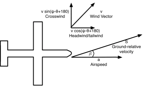
Fig. 1. Diagram showing the components affecting ground-relative

movement of the UAS platform used in Eq. (1). The ground-relative velocity is the summation of the airspeed and plane relative wind vectors.

to improve wind speed estimates by having measurements of the true airspeed.

2.1 Best curve fitting

One method of retrieving information about the wind from a SMARTSonde flight is by fitting a curve to the UAS’s ground relative speed provided by the onboard GPS unit, which is called the best curve fitting method (BCF). This method is similar to the wind algorithm used by Reuder et al. (2009). The magnitude of the ground-relative speed, S, can be ex-pressed as

S2=(a+vcos(ψ−θ+180))2+(vsin(ψ −θ+180))2, (1) whereψis the airplane heading with north being 0◦,θis the wind direction using standard meteorological convention,a

is the airspeed of the aircraft, and v is the wind speed. A diagram showing the components of Eq. (1) is provided in Fig. 1. For this method,acan be treated as a constant if the aircraft is flying with a constant throttle and pitch. Although it must be noted that the true airspeed will vary slightly as the angle of attack changes dynamically, a mean airspeed over a circle flown by the UAS exists based on the mean angle of attack.

The values of S and the ground track angle are known since they are recorded every second from the GPS. It is im-portant to note that ground track angle is different from the heading, ψ, as the difference between them is the sideslip angle,β, as shown in Fig. 1. However, it is possible to back out the true heading of the aircraft from the ground track an-gle, since the ground track vector is the summation of the air-speed and wind vectors. Based on vector math and trigonom-etry from Fig. 1,βcan be expressed as

β =tan−1

_v_sin_(ψ ₋_θ₊₁₈₀₎

vcos(ψ−θ+180)+a

, (2)

(4)

a Airspeed v cos(ψ-θ+180) Headwind/tailwind v sin(ψ-θ+180)

Crosswind

v Wind Vector

S Ground-relative

velocity

β

Fig. 1: Diagram showing the components affecting ground-relative movement of the UAS platform

used in Eq. (1). The ground-relative velocity is the summation of the airspeed and plane relative

wind vectors.

0 50

100 150

200

−50 0 50 100 150 200

0 50 100 150 200 250 300 350

X (m) Y (m)

Z (m)

12 14 16 18 20 22

Fig. 2: A trace of a flight path on 17 November 2011. The shading indicates the SMARTSonde’s

ground relative speed (m s

−1

). On this day, the wind direction was northerly, becoming more easterly

with height. The winds affect on the aircraft’s speed can be seen, as the aircraft moved faster with a

tailwind and slower with a headwind.

17

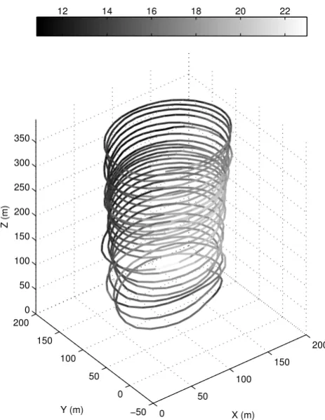
Fig. 2. A trace of a flight path on 17 November 2011. The

shad-ing indicates the SMARTSonde’s ground relative speed (m s−1). On this day, the wind direction was northerly, becoming more east-erly with height. The winds affect on the aircraft’s speed can be seen, as the aircraft moved faster with a tailwind and slower with a headwind.

where the numerator is the crosswind and the denominator is the summation of the airspeed and the headwind.ψis found by taking the difference between the ground track angle and

β. This relationship between the ground track with ψ can be used in the iterative process of determining the horizontal wind through the polynomial curve fitting.

With this information, a polynomial curve fitting can be performed to determine the values ofa,v, andθ. While the fitting may be done as frequently as desired, it may not pro-vide an accurate estimate of the wind speed and direction if the analyzed dataset is windowed too narrowly. Ideally, the dataset would contain a large number of data points over a wide range ofψ. Generally, the fitting is performed each time the aircraft completes a circle, providing the entire range of

ψthat is needed for a representative fit of Eq. (1) to the data. To illustrate the application of the curve fitting method, SMARTSonde data from a helical ascent are depicted in Fig. 2. On this particular day, the prevailing winds were northerly. When the aircraft travels north, the headwind de-creases the relative speed. Conversely, the ground-relative speed of the SMARTSonde increases when flying

0 100 200 300 400

12 13 14 15 16 17 18 19 20 21

Heading (degrees)

Ground Relative Speed (m s

−

1 )

v

a

θ

Fig. 3: Example fitting of the equation in the BCF. This corresponds to the circle between 207 m and

218 m above ground level (AGL). The curve indicates the best fit of Eq. (1) and the circles represent

the data from the GPS unit. Airspeed (

a

) is marked by the solid line, wind speed (

v

) is noted by the

arrows, and wind direction (

θ

) is shown by the dash-dotted line.

0 2 4 6

50 100 150 200 250 300 350 400

Wind Speed (m s

−1

)

Height (m)

Wind Profile on 11/17/11

N E S W N

50 100 150 200 250 300 350 400

Wind Direction

Height (m)

Fig. 4: Derived wind profile by using the BCF on the flight shown in Fig. 2.

18

Fig. 3. Example fitting of the equation in the BCF. This corresponds

to the circle between 207 and 218 m a.g.l. The curve indicates the best fit of Eq. (1) and the circles represent the data from the GPS unit. Airspeed (a) is marked by the solid line, wind speed (v) is noted by the arrows, and wind direction (θ) is shown by the dash-dotted line.

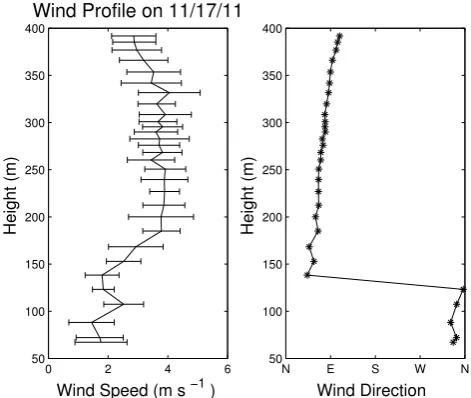
southward. Each circle in the flight can be individually ex-amined using the BCF. Equation (1) is fitted to the instanta-neous ground-relative velocities. A sample fitting of the data from one particular circle is shown in Fig. 3. By applying this fitting, the wind speedvand wind directionθfor the av-erage height of the aircraft during the circle is retrieved. This fitting is applied to every circle during the SMARTSonde’s ascent so that a wind profile of the PBL can be constructed, as shown in Fig. 4.

The aircraft does not need to fly in a circle to utilize the BCF. The fitting could work with most patterns as long as the airplane changes heading throughout the flight. However, the algorithm is able to provide the most frequent and accurate updates of a wind estimate when a circular flight path is used.

2.2 No-flow-sensor method

By using Nelder–Mead optimization (Nelder and Mead, 1965), the wind speed and direction can be retrieved through an alternative method. This method was originally proposed by Mayer et al. (2012) as the “no-flow-sensor”. Similar to the BCF, this algorithm utilizes an optimization scheme that re-lies only on the ground-relative velocity from the GPS unit. The airspeedais defined as

a = 1

n n X

i=1

||S(i)−W||, (3)

wheren is the number of the GPS measurements that are used in the optimization,S consists of the ground-relative velocity vector given by the GPS, andW is the wind vec-tor. All of the quantities are relative to the earth’s coordinate

(5)

0 100 200 300 400

12 13 14 15 16 17 18 19 20 21

Heading (degrees)

Ground Relative Speed (m s

−

1)

v

a

θ

Fig. 3: Example fitting of the equation in the BCF. This corresponds to the circle between 207 m and

218 m above ground level (AGL). The curve indicates the best fit of Eq. (1) and the circles represent

the data from the GPS unit. Airspeed (a) is marked by the solid line, wind speed (v) is noted by the

arrows, and wind direction (θ) is shown by the dash-dotted line.

0 2 4 6

50 100 150 200 250 300 350 400

Wind Speed (m s −1 )

Height (m)

Wind Profile on 11/17/11

N E S W N

50 100 150 200 250 300 350 400

Wind Direction

Height (m)

Fig. 4: Derived wind profile by using the BCF on the flight shown in Fig. 2.

18

Fig. 4. Derived wind profile by using the BCF on the flight shown

in Fig. 2.

system. Assuming perfect measurements and a constant air-speed and wind air-speed,S−W−a should be equal to zero. Since measurements are not perfect and the true wind fluctu-ates due to turbulence,S−W−adoes not necessarily equal zero; however, sincea andS are known values,W can be solved. To accomplish this, a standard deviation quantity,σ, is defined by

σ = 1

n n X

i=1

(||S(i)−W|| −a)2, (4)

which is minimized using a Nelder–Mead optimization scheme.

For the wind retrievals in this study, 151 GPS-derived val-ues are used in the optimization scheme. This number of ground-relative velocities is based on experimentation with different sample sizes. Since the GPS measurements are sam-pled at 5 Hz, this corresponds to around 30 s of flight time. Using a lower number of points,n, the wind data become noisy. With a larger sample size, small changes in the wind vector with height are not resolved. To date, the u and v

components of the wind have been reliably calculated for SMARTSonde flights using this method. However, due to the fact that thewcomponent is typically smaller than the noise in the GPS data, the vertical wind has not been resolved using this method.

Utilizing the no-flow-sensor, the wind speed can be esti-mated whenever the aircraft is maintaining a constant air-speed. The aircraft could be following any flight pattern, along a straight path or with many turns. The frequency of independent estimates of the wind speed is a function of the number of points used in the optimization scheme. This quantity may vary depending on the platform and the accu-racy of the GPS receiver.

2.3 Paparazzi wind algorithm

The Paparazzi autopilot program used by the SMARTSonde for autonomous flight provides an estimate of the wind speed and direction at the flight level. These values are reported ev-ery ten seconds. However, the wind algorithm in use with the autopilot software is not well documented. It uses some form of the no-flow-sensor methodology discussed above, but the number of points,n, that are used in the optimization are not reported. Paparazzi provides the only real-time estimate of the wind speed, as the other algorithms are used to process the data after the flights are complete. Typically, the estimate of the wind speed from the Paparazzi are erratic for∼30 s after the aircraft begins autonomous flight, while the other al-gorithms worked well during this time interval. A relatively accurate first guess would minimize the computing time and iterations needed to solve for the wind vector.

3 Algorithm performance and comparison

3.1 Comparison with rawinsonde

The three wind algorithms have been used to derive wind measurements for profiles of the PBL for comparison with a nearby rawinsonde and Mesonet station. The rawinsonde wind profiles used for comparison were from Norman, Ok-lahoma (OUN). Rawinsonde wind measurements are speci-fied to be accurate to within 1 m s−1for eachuandv com-ponent. The upper-air station is located less than a kilome-ter away from where the SMARTSonde flights for this study were conducted. The ground near the rawinsonde site is rel-atively flat, so terrain effects are minimal. Therefore, the rawinsonde observations are expected to be representative of the SMARTSonde observations. While the times of the radiosonde launches did not exactly match the times of the SMARTSonde profiles, the profiles compared were always within 2 h of each other.

The Oklahoma Mesonet consists of 110 stations through-out the state that measure air temperature, humidity, baro-metric pressure, wind speed and direction, rainfall, solar ra-diation, and soil temperatures (Brock et al., 1995; McPherson et al., 2007). The National Weather Center (NWC) Mesonet was used for additional comparison. The Mesonet station is maintained by the Oklahoma Climatological Survey (OCS); data are archived for public use with one minute resolution. The main advantage of using the NWC Mesonet observation is that the wind data, which is measured at 10 m a.g.l. (above ground level), at the moment of the SMARTSonde’s takeoff can be used for comparison. This shows if the 10 m wind changes significantly between the rawinsonde observation time and the time of the SMARTSonde flight. Wind speed and direction measurements from the NWC Mesonet station are accurate within 0.3 m −1and 3◦, respectively.

(6)

0 5 10

0 100 200 300 400 500 600

Speed (m s −1)

Height (m)

N E S W N

0 100 200 300 400 500 600

Direction (degrees)

Height (m)

Flight Time: 23:00Z

NFS PPRZ BCF OUN NWC

(a)

0 5 10

0 100 200 300 400 500

Speed (m s −1)

Height (m)

N E S W N

0 100 200 300 400 500

Direction (degrees)

Height (m)

Flight Time: 00:10Z

(b)

0 5 10

0 100 200 300 400 500 600

Speed (m s −1)

Height (m)

N E S W N

0 100 200 300 400 500 600

Direction (degrees)

Height (m)

Flight Time: 23:00Z

(c)

0 5 10

0 100 200 300 400 500

Speed (m s −1)

Height (m)

N E S W N

0 100 200 300 400 500

Direction (degrees)

Height (m)

Flight Time: 22:36Z

(d)

Fig. 5: Four examples of typical wind profiles using the different algorithms compared against the

NWC Mesonet observation at 10 m (NWC, black square) and the rawinsonde (OUN, solid black line

with asterisks). NFS is the no-flow-sensor (red line), PPRZ is the paparazzi output (green line), BCF

is the best curve fitting method (blue line).

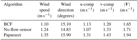
Table 1: Root mean squared errors (RMSE) for algorithms compared to rawinsonde observations for

all flights within 1 hour of rawinsonde launch time at heights above 300 m AGL

Algorithm Wind Speed Wind Direction u-comp v-comp |V|

(m s−1) (degrees) (m s−1) (m s−1) (m s−1)

BCF 1.10 15.10 1.13 1.20 1.65

No-flow-sensor 1.24 14.83 1.07 1.33 1.71

Paparazzi 1.35 15.90 1.31 1.43 1.94

19

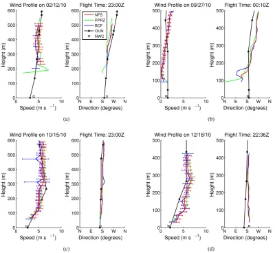
Fig. 5. Four examples of typical wind profiles using the different algorithms compared against the NWC Mesonet observation at 10 m (NWC,

black square) and the rawinsonde (OUN, solid black line with asterisks). NFS is the no-flow-sensor (red line), PPRZ is the paparazzi output (green line), BCF is the best curve fitting method (blue line).

The great majority of the 60 helical ascent flights con-ducted for this study occurred during periods when the synoptic-scale forcing was weak, absent of nearby frontal zones that could quickly change the PBL wind profile. Thus, conditions during the balloon launch should be similar to conditions during SMARTSonde flights, provided the two times are within a few hours of each other. Hence, it is rea-sonable to make direct comparisons between rawinsonde and SMARTSonde observations.

Shown in Fig. 5 are four typical wind profiles calculated using the three methods mentioned above. They are com-pared with observations from the Norman sounding (OUN) and the NWC Mesonet station. Note that the rawinsonde data are for the official launch time, 00:00 UTC, for all of the cases shown. However, the sondes are usually observed being launched earlier, at 23:00 UTC. Figure 5a depicts an event on 12 February 2010 when there was a noticeable wind direction shift from southerly to westerly between 300–500 m a.g.l. Based on the 925 mb map and soundings (not shown), this

wind shift was associated with an elevated mixed layer mov-ing over the cooler air near the surface. All of the wind data produced using the SMARTSonde’s algorithms agreed well with the rawinsonde observation. Another wind shift can also be seen in Fig. 5b. On this day, the winds were much lighter than the previous case, but both the rawinsonde and the wind algorithms still captured the low-level wind shear. In Fig. 5c, a noticeable feature was the weaker winds that were ob-served below 100 m a.g.l. This demonstrates that the algo-rithms are capable of retrieving weaker winds closer to the ground when the SMARTSonde begins a helical ascent at a low altitude. In the final example shown in Fig. 5d, once again weaker winds are observed near the surface. This flight took place∼30 min prior to the rawinsonde launch. Below 200 m a.g.l., the SMARTSonde and rawinsonde observations differ in wind direction. However, the SMARTSonde’s low-est observation from all three algorithms closely matches the wind direction at the NWC Mesonet at the takeoff time.

(7)

The four example plots comparing algorithm output against the sounding, as well as the many other compar-isons not shown here, generally illustrate good agreement between the rawinsonde observations and the different wind algorithms. Differences in wind profiles from the UAS and rawinsonde can be attributed to unreliable rawinsonde data below 300 m as well as evolution of the PBL wind profile during the evening transition period between rawinsonde and UAS observations. To better determine the accuracy of the algorithms, error statistics were calculated from all of the flights that took place within an hour of a rawinsonde being launched.

Table 1 provides the root mean squared errors (RMSE) between the rawinsonde wind data and UAS retrievals us-ing 22 rawinsonde and UAS profiles. Since rawinsonde wind observations under 300 m a.g.l. are typically unreliable, data below this height were not used in the computation of er-ror statistics in Table 1. The last column,|V|, is the mag-nitude of the vectorized RMSE for the wind, utilizing the vector addition of theuandv error components. Based on these numbers, both the no-flow-sensor and BCF provide measurements more similar to the rawinsonde than the Pa-parazzi algorithm in nearly every category. While the BCF has a lower error for the wind speed, the estimate of the wind direction from the no-flow-sensor has a lower RMSE. Both could be used to measure the 2-D wind vector with nearly identical errors. The RMSE for each of the wind components is slightly larger than the error for the rawinsonde system, which is 1 m s−1for uandv. This is not surprising consid-ering that the rawinsonde observations have error themselves and the winds may change slightly between the measurement times.

Overall, the three algorithms themselves were in good agreement with each other. No algorithm appeared to per-form drastically better than any other when compared against the rawinsonde, but each algorithm has its own advantages. The BCF provides the faster independent updates when the aircraft is flying in a circular pattern compared to the no-flow-sensor. Conversely, the no-flow-sensor method still works well when the aircraft is flying in a straight line, while the BCF does not work well in that condition.

3.2 Comparison with sodar

A Scintec XFAS sodar operates on the roof of the NWC and offers yet another wind dataset for comparison. The sodar provides 10 m vertical resolution estimates of the wind vector averaged over a 15 min time span. The lowest range gate is 30 m above the instrument and retrievals can provide data up to 400 m under ideal conditions, although the typical range is 200 m. The maximum height range varies drastically de-pending on atmospheric conditions and noise levels of the environment. Wind speed and direction measurements are specified to be accurate within 0.3 m s−1and 1.5◦. However, measurement quality is sensitive to the signal-to-noise ratio.

Table 1. Root mean squared errors (RMSE) for algorithms

com-pared to rawinsonde observations for all flights within 1 h of rawin-sonde launch time at heights above 300 m a.g.l.

Algorithm Wind Wind u-comp v-comp |V|

speed direction (m s−1) (m s−1) (m s−1) (m s−1) (degrees)

BCF 1.10 15.10 1.13 1.20 1.65

No-flow-sensor 1.24 14.83 1.07 1.33 1.71 Paparazzi 1.35 15.90 1.31 1.43 1.94

Given its continuous data stream and its spatial resolution near the ground, wind measurements from the NWC sodar are well suited for validating wind retrievals from SMART-Sonde flights.

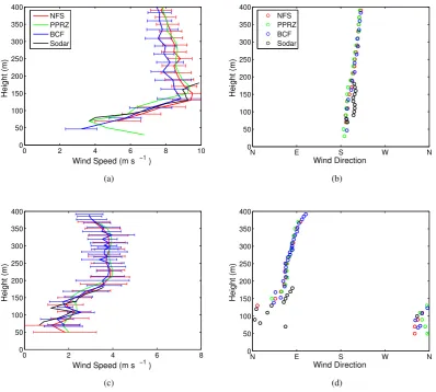
A series of flights were conducted on the mornings of 31 October and 17 November 2011 during the morning tran-sition of the boundary layer. The data from several of the flights and the sodar are shown in Fig. 6. On the morning of 31 October, a weak LLJ was observed by the SMARTSonde with a peak wind speed around 150 m a.g.l. Below this, there was an area of strong wind shear. Although the sodar did not retrieve a wind estimate much above 150 m a.g.l., the winds below this height agreed very well with those derived from the SMARTSonde flight. Concurrently, there was good agreement between both the sodar and SMARTSonde wind observations during the morning of 17 November. The wind speed increased rapidly with height from 100 to 200 m a.g.l., as shown with measurements from both instruments. Al-though there are some differences in the observed wind di-rection between the two profiles, both tended to show the wind shifting from northerly to more easterly with height. Due to technical problems with the sodar, there have only been limited opportunities for comparisons between the in-struments so far; however, observations visually have shown good agreement.

4 Example application

4.1 Calculating the Richardson number

Since the SMARTSonde is capable of measuring both the wind and thermodynamic variables, it is possible to cal-culate the gradient Richardson number (Ri). The gradient Richardson number is defined as

Ri=

g θ

∂θ ∂z

∂u ∂z

2

+

∂v ∂z

2, (5)

wheregis gravity,θis potential temperature,∂θ_∂z is the verti-cal potential temperature gradient,∂u_∂z is the vertical gradient of the zonal wind, and∂v_∂zis the vertical gradient of the merid-ional wind. Ri is a measure of the dynamic instability and can

(8)

0 2 4 6 8 10

0 50 100 150 200 250 300 350 400

Height (m)

NFS PPRZ BCF Sodar

(a)

N E S W N

0 50 100 150 200 250 300 350 400

Wind Direction

Height (m)

NFS PPRZ BCF Sodar

(b)

0 2 4 6 8

0 50 100 150 200 250 300 350 400

Height (m)

(c)

N E S W N

0 50 100 150 200 250 300 350 400

Wind Direction

Height (m)

(d)

Fig. 6: Comparisons of wind profiles from aScintec sodar (black) with derived wind speeds and

directions from SMARTSonde flights. Algorithm acronyms in the legend are same as in Fig. 5. Data

from a) and b) were taken on 31 October 2011 at 10:15 local time (LT) while data from c) and d)

were taken on 17 November 2011 at 8:36 LT.

20

Fig. 6. Comparisons of wind profiles from a Scintec sodar (black) with derived wind speeds and directions from SMARTSonde flights.

Algorithm acronyms in the legend are same as in Fig. 5. Data from (a) and (b) were taken on 31 October 2011 at 10:15 LT, while data from

(c) and (d) were taken on 17 November 2011 at 08:36 LT.

be used to indicate the formation of turbulence. When Ri is less than a critical Richardson number, the flow is viewed as being dynamically unstable, allowing turbulence to de-velop or persist. If Ri is greater than the critical Richardson number, then the flow is dynamically stable and turbulence is expected to decay. In literature, the value of the critical Richardson number varies from 0.2–1 or higher (Galperin et al., 2007), but the value is usually taken as 0.25 according to The Glossary of Meteorology of the American Meteoro-logical Society.

Vertical profiles of Ri can be calculated through finite dif-ferencing ofθ,u, andvwith height. Although the SMART-Sonde provides observations with high spatial resolution, the wind observations can be noisy with height. To reduce this effect on the calculation of the approximated gradient Richardson number, especially over short height intervals when1zbecomes small (i.e., less than 10 m), sets of three consecutive wind observations are averaged together, effec-tively creating one usable measurement for each set. After

this averaging, Ri can be calculated between each measure-ment. Consequently the vertical resolution of Ri varies based on ascent rate, with lower resolution measurements when the aircraft is ascending quicker.

4.2 Observations from 6 March 2011

Four consecutive flights were conducted on the morning for 6 March 2011 to observe the early morning transition of the PBL. Sunrise (06:53 LT – local time) occurred approx-imately 30 min before the first flight. Thereafter, each flight took place approximately 30 min apart to allow the boundary layer to develop and change substantially between each pro-file. During the first two flights, the SMARTSonde ascended at a slow rate in order to sample the near-surface thermody-namic structure with high vertical resolution. The SMART-Sonde ascended at a faster rate to penetrate the developing boundary layer during the last flights.

As the morning progressed, the depth of the convective boundary layer increased, as indicated by the increasing

(9)

2720 274 276 278 280 282

50 100 150 200 250 300

Potential Temperature (K)

Height (m)

07:18 07:50 08:25 08:59

(a)

1 1.5 2 2.5 3 3.5

0 50 100 150 200 250 300

Specific Humidity (g kg −1)

Height (m)

(b)

0 5 10

0 50 100 150 200 250 300

Speed (m s −1)

Height (m)

N E S W N

0 50 100 150 200 250 300

Direction

Height (m)

(c)

0 2 4 6 8 10

0 50 100 150 200 250 300

Gradient Richardson Number Profile

Richardson Number

Height (m AGL)

(d)

Fig. 7: SMARTSonde observations of the morning of 6 March 2011 from four sequential flights

after sunrise. Provided is a) potential temperature, b) specific humidity, c) wind profile using the

BCF method, and d) computed Richardson number. Local times for each flight is provided in the

legend. Sunrise occurred at 6:53 LT.

21

Fig. 7. SMARTSonde observations of the morning of 6 March 2011 from four sequential flights after sunrise. Provided is (a) potential

temperature, (b) specific humidity, (c) wind profile using the BCF method, and (d) computed Richardson number. Local times for each flight is provided in the legend. Sunrise occurred at 06:53 LT.

height of the inversion shown in Fig. 7a. For the first 90 min after sunrise, the depth of the convective boundary layer in-creased at a slow pace, growing to be only slightly less than 100 m deep by 08:25 LT, as evidenced by the inversion. Af-terwards, however, the rate of growth of the PBL drastically increased and reached a depth of about 200 m by 08:59 LT. This initial slow growth of the PBL followed by quick growth agrees well with past studies (White et al., 2002; Fisch et al., 2004). The depth of the PBL can be tracked by the moisture profiles in Fig. 7b, as the depth of the well-mixed moisture increases throughout the morning. In successive flights, the layer of air above the PBL in the entrainment zone cooled in time due to a negative heat flux as cool air from the sur-face is mixed upward and warmer air is mixed toward the surface, which agrees with results from Young et al. (2000) and Sullivan et al. (1998). Although it is difficult to draw def-inite conclusions from surface and upper air maps, there may be some weak cold, dry air advection occurring above the surface modifying the thermodynamic profile.

The wind profiles derived from the best-curve fitting method are shown in Fig. 7c. Wind profiles from the first three flights showed good agreement with each other. They each indicated a weak LLJ with a wind maximum of ∼8 m s−1 at 150 m a.g.l. with the wind speed decreasing above that height. By the last flight at 08:59 LT, the LLJ fea-ture had disappeared. At this time, the wind speeds below 200 m a.g.l. had decreased to∼4 m s−1 and were roughly constant with height above 50 m a.g.l. The decrease in wind speeds in this layer corresponds to the increase in the PBL depth during the same time interval between the third and fourth flights. Without a significant change in the synoptic-scale wind field, it can be assumed that the increase in the mixing depth is responsible for mixing down momentum from the LLJ. This is supported by the fact that the 10 m wind speed at the NWC Mesonet site increased by∼2 m s−1 between 07:30–09:00 LT (not shown). If wind speeds were measured down to ground level with the SMARTSonde or another instrument, it would be possible to calculate the mo-mentum fluxes using a modified integration approach from

(10)

Deardorff et al. (1980) explained by Bonin et al. (2013) from consecutive wind profiles close in time.

By combining both the wind and thermodynamic profiles, profiles of Ri have been calculated and are shown in Fig. 7d. Assuming the errors associated with both potential tempera-ture and wind are normally distributed, 10 000 realizations of

Ri were calculated using random values ofθ,u, andv

consis-tent with the mean and standard deviations for those values. The resulting mean value of Ri taken from the realizations is used as the reported value for the gradient Richardson num-ber, while the error bars are based on the standard deviation of the 5–95 % confidence interval of the realizations. Real-izations for which the wind shear is below 0.01 s−1were re-moved. Otherwise, estimates of Ri would become unrealis-tically large. This is particularly noticeable during the last flight at 150 m where the wind shear is almost nonexistent. For this case, the denominator in Eq. (5), approaches zero and Ri becomes very large.

During the first three flights, Ri below 120 m a.g.l. was mostly determined to be at or below 0.25. This value is pri-marily attributed to the strong shear associated with the bot-tom of the LLJ, before the momentum mixed downward. De-spite the strong static stability, turbulence may be produced at these heights due to the strong shear. During all of the flights, there was an increase in Ri at 150 m. This is likely due to the strong static stability and weak wind shear during the first three flights, and very weak wind shear with static stability during the fourth flight. This example shows the usefulness of having profiles of both thermodynamic and dynamic quan-tities of the PBL within∼30 min of each other.

5 Conclusions

Overall, the three algorithms that were tested with the SMARTSonde platform provided accurate results when com-pared with proximity rawinsonde and sodar observations. While the no-flow-sensor and BCF performed similarly, both seemed to provide more accurate estimates than the output from the Paparazzi autopilot software. Either algorithm could be used to measure the winds within 1.25 m s−1and 16◦of rawinsonde observations. However, the fitting method pro-vides the fastest independent observations when the aircraft is flying in small circles, which was the case for the flights provided in this study. The no-flow-sensor is the preferred al-gorithm to use when a limited number of turns are executed, since this algorithm does not require a change in heading for accurate retrievals.

These methods are used to accurately retrieve the 2-D wind vector from a low-cost UAS platform utilizing only data from an onboard GPS. Additional sensors, such as an IMU or probes with various dynamic and static pressure holes, could be incorporated onto the SMARTSonde or other UASs for faster and more accurate measurements. However, these sen-sors would significantly increase the cost of the platform.

It has been demonstrated that the wind estimates obtained can be combined with the thermodynamic profiles measured during the SMARTSonde flights to calculate the Richardson number with 50 m vertical resolution within the PBL. Ad-ditionally, the ability to make sequential wind and thermo-dynamic profiles with a vertical resolution of∼10 m allows for closer examination of other interesting processes, such as the development of a LLJ in the evening or quantifying low-level wind shear in a pre-storm environment. UASs are unique platforms capable of taking high-resolution thermo-dynamic and thermo-dynamic measurements, and can be used to ex-amine many atmospheric processes in a new way.

Acknowledgements. We thank our colleagues who have helped with the collection of the data, including all of those who have assisted in the development of the SMARTSonde. We are especially grateful to Wayne Shalamunec for piloting the SMARTSonde and putting many hours into the project, and to the Central Oklahoma Radio Control Society for allowing use of their airfield for flights. We would like to thank Alan Shapiro for his helpful comments. We are grateful for the anonymous reviewers’ comments, which have improved the quality of this article. Funding to support the development of SMARTSonde has been provided by the University of Oklahoma (OU) Advanced Radar Research Center (ARRC) and through a grant provided by the National Oceanic Atmospheric Administration (NOAA) National Severe Storms Laboratory (NSSL).

Edited by: A. Benedetto

References

Barthelmie, R., Grisogono, B., and Pryon, S.: Observations and sim-ulations of diurnal cycles of near-surface wind speeds over land and sea, J. Geophys. Res., 101, 21327–21337, 1996.

Bonin, T., Chilson, P. B., Zielke, B., and Fedorovich, E.: Observa-tions of early evening boundary-layer transiObserva-tions using a small unmanned aerial system, Bound.-Lay. Meteorol., 146, 119–132, 2013.

Bonner, W. D.: Climatology of the Low Level Jet, Mon. Weather Rev., 96, 833–850, 1968.

Brisset, P., Drouin, A., Gorraz, M., Huard, P.-S., and Tyler, J.: The Paparazzi solution, http://www.recherche.enac.fr/paparazzi/ papers 2006/mav06 paparazzi.pdf (last access: 18 Decem-ber 2012), 2006.

Brock, F. V., Crawford, K. C., Elliott, R. L., Cuperus, G. W., Stadler, S. J., Johnson, H. L., and Eilts, M. D.: The Oklahoma Mesonet: A Technical Overview, J. Atmos. Ocean. Tech., 12, 5–19, 1995. Chilson, P. B., Gleason, A., Zielke, B., Nai, F., Yeary, M.,

Klein, P. M., and Shalamunec, W.: SMARTSonde: A Small UAS platform to support radar research, in: 34th Confer-ence on Radar Meteorology, Extended abstract 12B.6, avail-able at: http://ams.confex.com/ams/34Radar/techprogram/paper 156396.htm, American Meteorological Society, Boston, Mass., 2009.

(11)

Deardorff, J., Willis, G., and Stockton, B.: Laboratory Studies of the Entrainment Zone of a Convectively Mixed Layer, J. Fluid Mech., 100, 41–64, 1980.

Dias, N., Gonc¸alves, J., Freire, L., Hasegawa, T., and Malheiros, A.: Obtaining Potential Virtual Temperature Profiles, Entrain-ment Fluxes, and Spectra from Mini Unmanned Aerial Vehicle Data, Bound.-Lay. Meteorol., 145, 93–111, 2012.

Emeis, S., Harris, M., and Banta, R. M.: Boundary-layer anemom-etry by optical remote sensing for wind energy applications, Me-teorol. Z., 16, 337–347, 2007.

Endlich, R., Ludwig, F., Bhumralkar, C., and Estoque, M.: A Di-agnostic Model for Estimating Winds at Potential Sites for Wind Turbines, J. Appl. Meteorol., 21, 1441–1454, 1982.

Fisch, G., Tota, J., Machado, L., Silva Dias, M., da F. Lyra, R., No-bre, C., Dolman, A., and Gash, J.: The convective boundary layer over pasture and forest in Amazonia, Theor. Appl. Climatol., 78, 47–59, 2004.

Galperin, B., Sukoriansky, S., and Anderson, P. S.: On the critical Richardson number in stably stratified turbulence, Atmos. Sci. Lett., 8, 65–69, 2007.

Holland, G., Webster, P., Curry, J., Tyrell, G., Gauntlett, D., Brett, G., Becker, J., Hoag, R., and Vaglienti, W.: The Aerosonde Robotic Aircraft: A New Paradigm for Environmental Observa-tions, B. Am. Meteorol. Soc., 82, 889–901, 2001.

Holton, J. R.: The Diurnal Boundary Layer Wind Oscillation Above Sloping Terrain, Tellus, 19, 199–205, 1967.

Houston, A., Argrow, B., Elston, J. S., Lahowetz, J., Frew, E., and Kennedy, P. C.: The Collaborative Colorado-Nebraska Un-manned Aircraft System Experiment, B. Am. Meteorol. Soc., 93, 39–54, 2012.

Kondragunta, S., Lee, P., McQueen, J., Kittaka, C., Prados, A., Ciren, P., Laszlo, I., Pierce, R., Hoff, R., and Szykman, J.: Air Quality Forecast Verification Using Satellite Data, J. Appl. Me-teorol. Clim., 47, 425–442, 2008.

Lin, P.-H.: Observations: The First Successful Typhoon Eyewall-Penetration Reconnaissance Flight Mission Conducted by the Unmanned Aerial Vehicle, Aerosonde, B. Am. Meteorol. Soc., 87, 1481–1483, 2006.

Martin, S., Bange, J., and Beyrich, F.: Meteorological profiling of the lower troposphere using the research UAV “M2AV Carolo” Atmos. Meas. Tech., 4, 705–716, doi:10.5194/amt-4-705-2011, 2011.

Mayer, S., Hattenberger, G., Brisset, P., Jonassen, M., and Reuder, J.: A ’no-flow-sensor’ Wind Estimation Algorithm for Un-manned Aerial Systems, Int. J. Micro Air Vehicl., 4, 15–29, 2012. McPherson, R. A., Fiebrich, C. A., Crawford, K. C., Kilby, J. R., Grimsley, D. L., Martinez, J. E., Basara, J. B., Illston, B. G., Morris, D. A., Kloesel, K. A., Melvin, A. D., Shrivastava, H., Wolfinbarger, J. M., Bostic, J. P., Demko, D. B., Elliott, R. L., Stadler, S. J., Carlson, J., and Sutherland, A. J.: Statewide Moni-toring of the Mesoscale Environment: A Techincal Update on the Oklahoma Mesonet, J. Atmos. Ocean. Tech., 24, 301–321, 2007.

Nelder, J. and Mead, R.: A simplex method for function minimiza-tion, Comput. J., 7, 308–313, 1965.

Parish, T. R. and Oolman, L. D.: On the Role of Sloping Terrain in the Forcing of the Great Plains Low-Level Jet, J. Atmos. Sci., 67, 2690–2699, 2010.

Premerlani, W. and Bizard, P.: Direction Cosine Matrix IMU: The-ory, gentlenav.googlecode.com/files/DCMDraft2.pdf (last ac-cess: 18 December 2012), 2009.

Reuder, J., Brisset, P., Jonassen, M., M¨uller, M., and Mayer, S.: The Small Unmanned Meteorological Observer SUMO: A new tool for atmospheric boundary layer research, Meteorol. Z., 18, 141– 147, 2009.

Seaman, N. L. and Michelson, S. A.: Mesoscale Meteorological Structure of a High-Ozone Episode during the 1995 NARSTO-Northeast Study, J. Appl. Meteorol., 39, 384–398, 2000. Shapiro, A. and Fedorovich, E.: Nocturnal Low-Level Jet over a

Shallow Slope, Acta Geophys., 57, 950–980, 2009.

Shuqing, M., Hongbin, C., Gai, W., Yi, P., and Qiang, L.: A Minia-ture Robotic Plane Meteorological Sounding System, Adv. At-mos. Sci., 21, 890–896, 2004.

Spiess, T., Bange, J., Buschmann, M., and V¨orsmann, P.: First appli-cation of the meteorological Mini-UAV ’M2AV’, Meteorol. Z., 16, 159–169, 2007.

Sullivan, P. P., Moeng, C.-H., Stevens, B., Lenschow, D. H., and Major, S. D.: Structure of the Entrainment Zone Capping the Convective Atmospheric Boundary Layer, J. Atmos. Sci., 55, 3042–3064, 1998.

van den Kroonenberg, A., Martin, T., Buschmann, M., Bange, J., and Vorsmann, P.: Measuring the Wind Vector Using the Au-tonomous Mini Aerial Vehicle M2AV, J. Atmos. Ocean. Tech., 25, 1969–1982, 2008.

van den Kroonenberg, A., Martin, S., Beyrich, F., and Bange, J.: Spatially-Averaged Temperature Structure Parameter Over a Heterogeneous Surface Measured by an Unmanned Aerial Vehi-cle, Bound.-Lay. Meteorol., 142, 55–77, 2012.

Wexler, H.: A Boundary Layer Interpretation of the Low-Level Jet, Tellus, 13, 368–378, 1961.

White, A., Templeman, B., Angevine, W., Zamora, R., King, C., Russell, C., Banta, R., Brewer, W., and Olszyna, K.: Regional contrast in morning transitions observed during the 1999 South-ern Oxidants Study Nashville/Middle Tennessee Intensive, J. Geophys. Res., 107, 4726–4737, 2002.

Williams, A. and Marcotte, D.: Wind Measurements on an maneu-vering twin-engine turboprop aircraft accounting for flow distor-tion, J. Atmos. Ocean. Tech., 17, 795–810, 2000.

Young, G. S., Cameron, B. K., and Hebble, E. E.: Observations of the entrainment zone in a rapitly entraining boundary layer, J. Atmos. Sci., 57, 3145–3160, 2000.