Multiresolution wavelet analysis applied to GRACE range-rate residuals

https://doi.org/10.5194/gi-8-197-2019

© Author(s) 2019. This work is distributed under the Creative Commons Attribution 4.0 License.

Multiresolution wavelet analysis applied to GRACE

range-rate residuals

Saniya Behzadpour1,2,*, Torsten Mayer-Gürr1, Jakob Flury2, Beate Klinger1, and Sujata Goswami3 1_{Graz University of Technology, Institute of Geodesy, Steyrergasse 30/III, 8010 Graz, Austria}

2_{Leibniz University Hanover, Institute of Geodesy, Schneiderberg 50, 30167 Hanover, Germany} 3_{Jet Propulsion Laboratory, NASA, Pasadena, CA, USA}

*_{Invited contribution by Saniya Behzadpour, recipient of the EGU Geodesy Outstanding Student Poster} and PICO Award 2018.

Correspondence:Saniya Behzadpour ([email protected]) Received: 26 November 2018 – Discussion started: 15 January 2019 Revised: 3 July 2019 – Accepted: 13 July 2019 – Published: 15 August 2019

Abstract. For further improvements of gravity field mod-els based on Gravity Recovery and Climate Experiment (GRACE) observations, it is necessary to identify the error sources within the recovery process. Observation residuals obtained during the gravity field recovery contain most of the measurement and modeling errors and thus can be con-sidered a realization of actual errors.

In this work, we investigate the ability of wavelets to help in identifying specific error sources in GRACE range-rate residuals. The multiresolution analysis (MRA) using discrete wavelet transform (DWT) is applied to decompose the resid-ual signal into different scales with corresponding frequency bands. Temporal, spatial, and orbit-related features of each scale are then extracted for further investigations.

The wavelet analysis has proven to be a practical tool to find the main error contributors. Besides the previously known sources such as K-band ranging (KBR) system noise and systematic attitude variations, this method clearly shows effects which the classic spectral analysis is hardly able or unable to represent. These effects include long-term signa-tures due to satellite eclipse crossings and dominant ocean tide errors.

1 Introduction

For more than 15 years, the Gravity Recovery and Climate Experiment (GRACE) satellite mission measured the time variation of Earth’s gravity field with high temporal and

spa-tial resolutions (Tapley et al., 2004). The mission was a trail-ing formation of two satellites, GRACE-A and GRACE-B, and provided the observation signals of intersatellite ranging, GPS tracking, the satellite attitudes, and nongravitational ac-celerations, which are required for the gravity field parameter estimation.

Based on these observations, various time-variable gravity models with monthly resolution were published by different analysis centers (e.g., Bettadpur, 2012; Dahle et al., 2012; Mayer-Gürr et al., 2016). The accuracy level of such mod-els has gradually increased in recent years; however, it has not reached the GRACE baseline accuracy computed through pre-launch simulations (Kim, 2000; Kim and Tapley, 2002). This results in an ongoing effort to understand the error con-tent of GRACE observations, as well as any inaccuracies in the physical and stochastic models used for processing GRACE data.

If the calibration parameters are correctly adjusted and the stochastic model fully describes the observation noise, it is expected that all of the mentioned errors are completely con-tained within the residuals. In reality, however, these errors might affect the gravity parameters due to imperfections in modeling. Therefore, residual analysis becomes a research topic as it is not only a way to study measurement and phys-ical modeling errors, but also helps to evaluate and improve the gravity field solutions.

The studies in this field have been conducted mainly on the theoretical residuals, which are the difference between the actual GRACE ranging observation and simulated obser-vation computed through force models. Ditmar et al. (2012) applied spectral analysis on theoretical residuals and showed that the major contributors to the noise budget at high fre-quencies are K-band ranging (KBR) sensor noise and in-accuracies in Earth’s assumed static gravity field at higher degrees. It also has been shown that uncertainties in back-ground models and errors in computed dynamic orbits con-tribute to low-frequency noise.

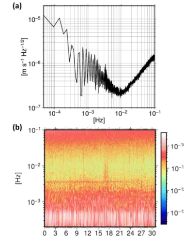
The main challenge in the spectral analysis of the residu-als is that several noisy signresidu-als and disturbances are known to be superimposed at each frequency. Furthermore, the anal-ysis is based on the assumption of the stationary behavior of these signals. However, in reality, most of these signals have nonstationary behavior, meaning that they have dynamic fre-quency components over time. Classical spectral analysis us-ing Fourier transforms only represents the frequency content of such signals (Fig. 1a) and does not provide any informa-tion about the time at which a signal at a specific frequency occurred or the duration for which it lasted (Keller, 2004). Consequently, in this framework, it is not possible to localize each component of the residuals in time for further statistical, spatial, or orbital analysis. The drawback of this framework draws our attention to spatiotemporal approaches, which in-corporate data analysis as well as geophysical model valida-tion (e.g., Dransch et al., 2010).

In an attempt to consider time variations in the sought-after signals, time–frequency methods can be applied to identify and localize the content of the nonstationary signals in the time and frequency domains simultaneously. The simplest method is the short-time Fourier transform (STFT), which is implemented by sliding a window throughout a signal and applying a Fourier transform to each windowed data seg-ment. The squared magnitudes of the STFT coefficients form a spectrogram, representing the variation of the signal’s spec-trum over time (Fig. 1b). The shape and length of the window function determines the fixed time and frequency resolution of the STFT. Due to this uniform time resolution for all fre-quencies, the STFT is limited to capturing time information on rapid changes in a signal as well as spectral information in its lower-frequency components.

To overcome STFT drawbacks, the wavelet analysis was introduced as a more effective technique for representation, decomposition, and reconstruction of nonstationary signals

Figure 1. (a)Power spectral density (PSD) and(b) spectrogram of the range-rate residuals from December 2008. Time–frequency methods can be applied to the residual time series to localize the time-variable frequency content.

(Keller, 2004). In contrast to STFT, the wavelet transform provides a better trade-off between time and frequency res-olution by using windows with shorter time spans at higher frequencies and windows with longer time spans at lower fre-quencies. The multiresolution analysis (MRA), introduced by Mallat (1989) and Meyer (1993), is an efficient imple-mentation of a wavelet transform for real signals. MRA can decompose a signal into multiscale components which can describe all time-variable structures in that signal.

The aim of this paper is to exploit the advantages of the wavelet transform to investigate the major contributors to GRACE range-rate residuals and ideally detect nonstation-ary noise sources in sensors and background models which cannot be observed with traditional spectral analysis. The re-sults of this study will further improve gravity field modeling based on GRACE data. In addition, they will be beneficial for the preparation of GRACE Follow-On data processing infrastructure. To reach this goal, we decompose the residual signal into three groups of scale and compare the character-istics of each group with known or supposed sources.

em-ployed method on the residuals are described. Finally, Sect. 5 presents the interpretation of results and a discussion.

2 Range-rate residuals from the ITSG-Grace2016 model

In this study, we use GRACE range-rate residuals obtained in the course of computing the ITSG-Grace2016 (Mayer-Gürr et al., 2016) gravity field model up to degree and order 60. Therefore, in order to introduce the residual signal, we briefly explain the processing chain of the model (Klinger et al., 2016).

In the ITSG-Grace2016 gravity field processing, high-precision kinematic orbits (Zehentner and Mayer-Gürr, 2013) with a sampling of 5 min and K-band intersatellite range rates with a sampling of 5 s serve as observations. Us-ing the approach of variational equations, dynamic orbits are computed for each day (Ellmer and Mayer-Gürr, 2017), and normal equations are set up with an arc length of 3 h. The ac-cumulated normal equations are then solved to estimate grav-ity parameters in terms of spherical harmonic coefficients, spanning from degree 2 up to degree 60. The background models used during the dynamic orbit integration are listed in Table 1.

In the course of the adjustment process, nongravity param-eters are also co-estimated for each day. These paramparam-eters in-clude the initial orbit states of both satellites, accelerometer scale factor matrices, accelerometer biases modeled by cubic splines with 6 h nodes, and daily gravity field variations up to degree and order 40.

It is worth mentioning that unlike in the standard GRACE monthly solutions, in ITSG-Grace2016 the correlations be-tween observations within a data block of 3 h are taken into account. For each observation type, a stochastic model of the observation noise is built under the assumption of stationar-ity. This model is estimated once per month directly from the observation residuals.

The weights for the different frequency components of the observations are determined through the residual power spec-tral density (PSD). This PSD is iteratively computed directly from the residuals through variance component estimation (VCE) (Koch, 1999). VCE is also used to estimate the rela-tive weights for the combination of different data types, i.e., kinematic orbits and range-rate observations. This modeling approach seems to appropriately separate the complex col-ored noise in the observations from the gravity signal; there-fore, we expect the residuals to contain most of the imperfec-tions caused by the instruments and background models.

3 Multi-resolution analysis (MRA)

The wavelet transformWf (u, s)of a signalf (t )∈L2(R),

Wf (u, s)= hf, ψu,si = ∞

Z

−∞

f (t )√1

sψ _t−u

s

dt, (1)

is the decomposition of that signal over a set of scaled and translated versions of a finite energy and normalized func-tion, the mother waveletψ.

For the wavelet transformWf (u, s), the translation param-eterudetermines the location of the wavelet in the time do-main, while the scale parametersis related to the frequency location. These parameters are continuous real values, there-fore an infinite number of coefficients are needed to describe a signal in this framework. In a practical implementation, it is convenient to discretize these parameters, as the real sig-nals are band limited. The usual choice is to follow aJ-scale dyadic discretization based on powers of 2. This transform is then called a discrete wavelet transform (DWT). For a signal with sampling frequency ofFS, the resulting coeffi-cientsd(j, n)can be interpreted as detailed subsignals at the scale 2j(1≤j≤J), corresponding to the frequency interval

[FS/2j+1, FS/2j]: d(j, n)=X

t

f (t )ψj,n(t ),

with ψ (j, n)=2−j/2ψ

_t−n2j

2j

; j, n∈_Z. (2) The approximation of the signal at the scaleJ, which cor-responds to the frequency interval[0, FS/2J+1]is also given by

a(J, n)=X

t

f (t )φJ,n(t ), (3)

whereφ (J, n) is the scaling function, associated with the wavelet functionψ (j, n).

The original signal can be reconstructed by adding all lay-ers of details up to decomposition scaleJ as well as the ap-proximation subsignal:

f (t )=X

n

a(J, n)φJ,n(t )+

X

j≤J

X

n

d(j, n)ψj,n(t ). (4)

Mallat (1989) showed that for a discrete signalf[n], any DWT on the orthonormal basis ofL2(R)could be

Table 1.Summary of ITSG-Grace2016 force models.

Perturbation Force model Reference

Earth’s static gravity field, trend, and annual oscillation GOCO05S Mayer-Gürr et al. (2015) Astronomical tides (Moon, Sun, planets) JPL DE421 Folkner et al. (2009)

Ocean tides EOT2011a Savcenko and Bosch (2012)

Nontidal atmosphere and ocean AOD1B RL05 Dobslaw et al. (2013)

Atmospheric tides (S1, S2) van Dam, Ray van Dam and Ray (2010)

Solid Earth tides IERS2010 Petit and Luzum (2010)

Pole tides IERS2010

Ocean pole tides IERS2010

Relativistic corrections IERS2010

h[n] =

₁

√

2φ _t

2

, φ(t−n)

, (5)

g[n] =

₁

√

2ψ _t

2

, φ(t−n)

. (6)

Mathematically, the convolution of the filter response with the discrete signal is expressed as follows:

a[p] =

∞

X

n=−∞

h[n−2p]f[n] =f ? h[2p], (7)

d[p] =

∞

X

n=−∞

g[n−2p]f[n] =f ? g[2p]. (8) The scaling function, defined by the filter coefficientsh[n], provides approximation coefficients a, which are also re-ferred to as low-pass output. The wavelet function, defined by the filter coefficients g[n], provides the detailed coeffi-cientsd, or alternatively the high-pass output. This decom-position step is followed by a factor 2 down-sampling of the output signals. According to Vetterli and Herley (1992), down-sampling cancels the aliasing between the resulting co-efficients. This is a necessary condition for recovery of the original signal with an inverse DWT.

A fast inverse DWT reconstructs the initial signalf[n]by up-sampling and filtering. The up-sampling operation is done by inserting zeroes between every other coefficients in the output signals a[n] andd[n]. The zero-padded coefficients

ˆ

a anddˆare then filtered by the corresponding inverse filters e

h[n]and_eg[n]:

f[n] = ˆa ?eh[n] + ˆd ?_eg[n]. (9) As described before, the DWT decomposes the original signal into an approximation subsignal and detailed subsig-nals. The MRA algorithm suggested by Mallat (1989) and Meyer (1993) calls for this decomposition to be repeated on the approximation subsignal, again yielding detailed subsig-nals and an approximation subsignal. The selection of the decomposition level depends on the initial size of the origi-nal sigorigi-nal, and the desired spectral and temporal resolution.

Figure 2.Three-level MRA decomposition tree, consisting of a high-pass filterg[n]and a low-pass filterh[n]followed by a down-sampling operator at each level.

Finally, the original signal can be represented by the approx-imation coefficients of the last decomposition level and the accumulated detailed coefficients of all decomposition lev-els. Figure 2 shows a three-level decomposition MRA algo-rithm.

We applied MRA using a discrete Daubechies wavelet transform with 20 vanishing moments (Daubechies, 1992) to decompose a monthly time series of residuals into eight different scales. The choice of the Daubechies wavelet is due to its usual application in signal detection and classification. The selection of a high vanishing moment is due to a high smoothness property of the resulting mother wavelet, leading to a better frequency localization in the millihertz (mHz) fre-quency band. Figure 3 shows scaling and wavelet functions for Daubechies-20 together with its corresponding decompo-sition and reconstruction conjugate mirror filters.

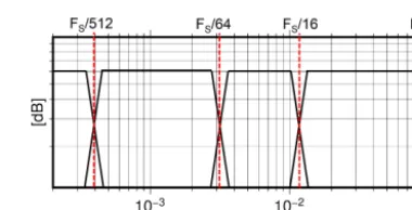
As shown in Fig. 4, we merged detailed coefficients into three major groups, defined approximately through three fre-quency subbands (Fig. 5):

Figure 3.Daubechies-20(a)scaling function,(b)wavelet function, (c)decomposition low-pass filter,(d)decomposition high-pass fil-ter,(e)reconstruction low-pass filter, and(f) reconstruction high-pass filter.

b. medium timescale details, containing the details at lev-els 4 to 5, corresponding to the frequency range from 3.125 up to 12.5 mHz;

c. long timescale details, containing the details at levels 6 to 8, corresponding to the frequency range from 0.391 up to 3.125 mHz.

Each group is then reconstructed into a time series of resid-uals using Eq. (9). Afterward, the time series are analyzed in three different domains. We have chosen the domains in such a way that they highlight specific characteristics of the error sources contained within the residual time series. They are the following.

Spectral/temporal domain. As mentioned in the first sec-tion, a spectrogram shows the variation of a signal’s en-ergy as a function of time and frequency. Another tool which can be used directly on the wavelet coefficients is the scalogram, in which the amplitude of the coeffi-cients are plotted as a function of the scale and transition parameters. In our analyses, we used spectrograms be-cause the interpretation of a signal in terms of frequency is more accessible than in terms of scale (Fig. 6). Spatial domain. Plotting each time series with respect to

the satellite ground track is useful to identify any fea-tures of geophysical origin in the data (Fig. 7).

Orbital domain. Plotting each time series as a function of satellite position and time reveals features related to the orbit geometry or instrument errors caused by orbital conditions. As the GRACE orbits are near-circular, the position of each satellite can be specified without loss of accuracy by the argument of latitude, ranging from

Figure 4.The proposed MRA scheme, implemented according to the characteristics of the residual signal.

Figure 5.The proposed MRA bandwidth division of the residuals with frequency samplingFSof 0.2 Hz.

−180 to 180◦. This domain represents the ascending Equator pass of the satellite at 0◦_{, the north pole at 90}◦_,

the descending Equator pass at 180 or−180◦_{, and then}

the south pole at−90◦(Fig. 8).

These analyses are carried out on the whole ITSG-Grace2016 time span (April 2002–June 2017). However, due to low data quality before 2004 and several data gaps and degraded quality of the measurements after 2016, these time periods are excluded from the illustrations. Highlights of this analysis are presented in the next section.

4 Results

To prove whether or not our applied method using the DWT is applicable to detect the error sources, we initially fo-cused on the investigation of known issues. For instance, it is known that the K-band system noise is dominant in the frequency range above 12.5 mHz. This frequency band cor-responds to the short timescale details of the residuals. The power of the noise in this band increases linearly with fre-quency. This is a result of the way the range-rate observations are derived from the range measurements by differentiation. Investigations by Ko et al. (2012) and Harvey et al. (2017) showed that the excessive high-frequency signatures in this band are highly correlated with low signal-to-noise (SNR) values of the K-band frequency observation by GRACE-B. Figure 9 compares these SNR values with the wavelet short timescale components, revealing this strong correlation.

Figure 6. Time–frequency analysis of (a) short timescale, (b) medium timescale,(c)long timescale, and(d)approximation components of the residual signal. Spectrograms are computed with a window length of 5 h for December 2008.

Figure 7. Spatial distribution of(a)short timescale,(b) medium timescale, (c)long timescale, and(d)approximation components of the residual signal. The values are plotted with respect to the GRACE-A ground track for December 2008.

the computed antenna offset correction are also expected to be found in the millihertz (mHz) frequency band. Our time– frequency analysis shows a similarity between the residuals in medium timescale and the angular acceleration variations derived from star camera observations (Fig. 10). The spatial pattern of the residuals related to the attitude variations ap-pears as horizontal bands (Fig. 7b), consistent with the results presented by Inácio et al. (2015).

These first investigations already show that our applied method is well suited to identify error sources. However, compared to the spectral analysis, the advantage of the im-plemented method of DWT is a better separation of super-imposed signals in frequencies lower than 12.5 mHz. This enabled the identification of (a) systematic errors caused by eclipse crossings of the satellites and (b) dominant ocean tide model errors, which are explained in the following sections. 4.1 Satellite eclipse crossings

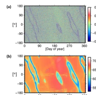
Analysis of the medium timescale details throughout the GRACE time span reveals long-term systematic signatures (Fig. 11a). Although the source of these errors is unknown, our investigation revealed a high correlation with the eclipse transit phases of GRACE-A and GRACE-B.

Figure 8. Orbital analysis of (a) short timescale, (b) medium timescale,(c)long timescale, and(d) approximation components of the residual signal. The values are plotted with respect to the GRACE-A argument of latitude for December 2008.

Figure 9. (a)Short timescale details of the residuals,(b) GRACE-B K-band SNR values. The values are plotted with respect to the GRACE-A argument of latitude for the time period 2009.

Each satellite passes through partial or full eclipse phases when it enters Earth’s shadow. Occasionally the Moon also casts a shadow on the satellites. The eclipse factor is defined as the fraction of the Sun’s light that reaches the satellite. It has a minimum value of zero if the satellite is in the umbra of the occulting body and a maximum value of one if the satellite is in direct sunlight. For a detailed calculation, the reader is referred to Montenbruck and Gill (2000).

Figure 10.Spectrograms of(a)GRACE-A pitch angular acceler-ation variacceler-ation and(b) medium timescale details of the residuals. The signal at 3.3 mHz, which according to Bandikova et al. (2012) is induced by magnetic torque attitude control, is clearly visible in the residuals for December 2008.

The GRACE formation mission started with GRACE-A as leading and GRACE-B as trailing satellite. After 3 years in orbit, the satellites had to exchange their positions to limit the damage on the K-band horn caused by atomic oxygen. This swap maneuver happened at the end of 2005. Before this time, eclipse crossing signature occurs when the pair entered sunlight. After the orbit swap maneuver in December 2005, when GRACE-B became the leading satellite, the signatures are visible when the pair enters the shadow area.

However, after the year 2011, these rules cannot explain the eclipse crossing signatures in the residuals as they appear in both entering and leaving shadow conditions with differ-ent intensities. The unstable thermal condition due to the dis-abled thermal controls might be a possible reason.

We compared the temperature measurements obtained from Level-1A High-Resolution Temperature data (HRT1A) for November 2008 and October 2011 with these signatures. It becomes obvious that there is a high correlation between the GRACE-B K-band antenna horn temperature variation and the disturbances during eclipse crossing events (Fig. 12). We suggest that the increasing temperature on the GRACE-B antenna horn may produce disturbances in the KGRACE-BR mea-surements. This hypothesis can be investigated in more detail once the complete GRACE Level-1A datasets become pub-licly available. From a gravity field recovery point of view, these eclipse crossing signatures can be interpreted as a tem-porary unmodeled signal in the range-rate measurements. 4.2 Ocean tide model

Errors in the background force models of temporal gravity field variations can be found in the long timescale details.

Figure 11. (a)Medium timescale details of the residuals and(b)the difference between GRACE-B and GRACE-A eclipse factors dur-ing the time period 2004–2010, plotted with respect to GRACE-A argument of latitude. The signatures are visible when the difference value is negative, i.e., GRACE-A is in the shadow and GRACE-B is in sunlight.(c)Medium timescale details of the residuals and(d)the difference between GRACE-B and GRACE-A eclipse factors dur-ing the time period 2011–2016, plotted with respect to GRACE-A argument of latitude. The signatures appear in both entering and leaving eclipse phase with different intensities. The gray areas indi-cate data gaps.

Due to the spatial nature of these errors and the periodicity of satellite passes over their source regions, different model errors are superimposed at the samencycles-per-revolution frequencies. Therefore, frequency or time–frequency plots cannot differentiate the dominant source from other influ-ences at this detailed scale.

The two main potential error sources at this scale are (a) in-accuracies in the employed ocean tide model EOT11a (Sav-cenko and Bosch, 2012) and (b) inaccuracies in the em-ployed nontidal atmosphere and ocean mass variation model, AOD1B RL05 (Dobslaw et al., 2013). To better understand the contributions of the individual models, we swap in alter-native models of the same forces and studied the resulting differences. This is best done in a closed-loop simulation, where other contributors to noise can be controlled. The sim-ulation is carried out for the time period 2008–2009, when GRACE delivered high-quality measurements and compar-ison of the actual data with the output of the simulation is more relevant. The following steps outline our employed simulation process:

1. Dynamic orbits are computed based on the background models mentioned in Table 1 with two exceptions. First, the FES2014 ocean tide model (Carrere et al., 2015) is substituted for the EOT11a model. Second, the AOD1B RL05 model and the van Dam–Ray atmospheric tide model (van Dam and Ray, 2010) were substituted with the AOD1B RL06 model. Compared to AOD1B RL05, the AOD1B RL06 model (Dobslaw et al., 2017) has un-dergone several improvements, amongst them a higher temporal resolution and the separation of nontidal and tidal signals, including atmospheric tides with 12 se-lected frequencies. Therefore, there was no need to con-sider a dedicated atmospheric tide model in the simula-tion employing AOD1B RL06.

2. Error-free observations for position, velocity, nongrav-itational accelerations, and the K-Band instrument are synthesized from these ideal orbits.

3. Realistic models of instrument noise are used to de-grade synthesized observations. White Gaussian noise with a standard deviation of 3 cm is added to the sim-ulated satellite positions. Accelerometer observations are degraded by white noise with a standard deviation of 0.3 nm s−2 in along-track and radial directions and 3 nm s−2in the cross-track direction. Star camera instru-ment noise is added as white Gaussian noise with a stan-dard deviation of 0.05 mrad to the orientation quater-nions. KBR instrument noise is computed by applying a differential filter to white Gaussian noise with a stan-dard deviation of 0.25 µm s−1_{, which is then added to} the simulated range-rate observations.

4. The final step is to recover a monthly gravity field us-ing the simulated degraded observations. To this end,

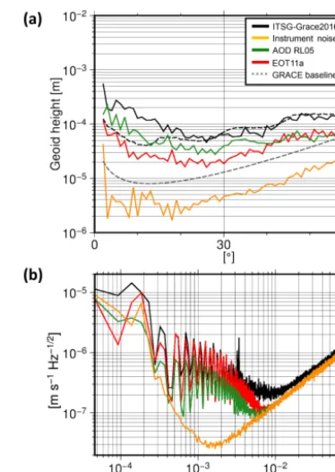
Figure 13. (a)RMS geoid heights per degree from simulated and real solutions with respect to the reference field GOCO05s.(b)PSD of the residuals from simulated and real data for February 2009.

the dynamic orbits are reintegrated using the artifi-cially degraded accelerometer observations and the sep-arate models under study, each in a dedicated scenario. The respective obtained residuals are then analyzed and compared.

4.2.1 Simulation scenario 1: propagated errors due to instrument noise

In the first scenario, the same background models as men-tioned in the first step of the simulation process are used to compute the reintegrated dynamic orbits. Therefore the re-sults only show the effects of instrument noise. As expected, the propagated noise is 1 order of magnitude smaller than the real residuals in frequency range from 0.391 up to 3.125 mHz (Fig. 13b) and obviously cannot explain the errors in the long timescale details. Analyzing the solution in terms of RMS geoid heights per degree with respect to the reference field GOCO05s, it can also be seen that the monthly solution based on instrument noise alone exhibits differences smaller than those of the GRACE baseline (Fig. 13a).

4.2.2 Simulation scenario 2: propagated errors due to AOD1B RL05

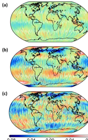
Figure 14. Spatial analysis of long timescale propagated errors from(a)AOD1B RL05 model and(b)EOT11a model, compared to(c)long timescale details of real residuals. The values are plotted with respect to the GRACE-A ground track for February 2009.

model and the van Dam–Ray atmospheric tide model (van Dam and Ray, 2010) were substituted for the AOD1B RL06 model. The simulated residual signal is then decomposed, and its long timescale components are compared to those ob-tained from real data. As shown in Fig. 13b, although the propagated errors have the same spectral behavior at fre-quency range from 0.391 to 3.125 mHz, their magnitude and spatial structure (Fig. 14a) cannot explain the real residuals. 4.2.3 Simulation scenario 3: propagated errors due to

EOT11a

In the third scenario, we study the contribution of the ocean tide model. To recover a gravity field in this scenario, the EOT11a ocean tide model is substituted for the FES2014 model. After decomposition of the simulated residual signal, its long timescale components are compared to the real data. These errors have comparable magnitude and spatial pattern (Fig. 14b) as those in the real data (Fig. 14c). This leads to the conclusion that the ocean tide model is the dominant error source at the long timescale detailed level.

These results showcase the capability of wavelet analy-sis in studying the signals due to geophysical processes in GRACE range-rate residuals. The implemented method effi-ciently finds structures in the signal which are not explicitly apparent in the PSD of the residuals. The wavelet analysis

proves to be an efficient tool in decomposing the background model errors and finding the most prominent sources.

5 Discussion and conclusions

The results presented in this paper show the advantages of using a DWT in analyzing the range-rate residuals from the ITSG-Grace2016 gravity field model. Several improvements in ITSG-Grace2016 resulted in a cumulative noise reduction of 20 %–40 % compared to its predecessor ITSG-Grace2014. The proposed analysis framework confirms known and re-veals previously unknown systematics in the residuals that allow for a specifically tailored parametrization in the grav-ity field retrieval.

We showed that the short timescale details of the residuals, equivalent to frequencies above 12.5 mHz, are dominated by KBR system noise. This is in agreement with the results pre-sented by Ko et al. (2012) and Ditmar et al. (2012). The errors in the satellite attitude determination were identified as a ma-jor contributor in the medium timescale details, equivalent to the frequency range from 3.125 to 12.5 mHz. This finding is consistent with the results presented by Inácio et al. (2015) and Bandikova et al. (2012).

Besides the previously known instrument error sources, long-term signatures due to eclipse transits of the satellites were identified. They appear as a bias term in the K-band range-rate observations. As this is a clearly deterministic ef-fect, its influence can be reduced by co-estimation of ad-ditional calibration parameters in the gravity field recovery process.

Analysis of the results from the implemented discrete wavelet transform brings new insights and a new understand-ing of the signals at the long timescale level. At this level, spectral analysis is unable to differentiate between the indi-vidual contributing sources, due to the nonstationary nature of the errors. Knowing that this scale level contains valu-able information about the time-varivalu-able gravity field sig-nal, we introduced nontidal mass variation and ocean tide models as the potential dominant sources. Comparing simu-lation results with the real data scenario, the EOT11a ocean tide errors are identified as the dominant error source within this scale. This means that using a more accurate ocean tide model can lower the residuals in this frequency band.

by using a wavelet base with higher vanishing moments and thus higher decomposition level.

Besides the range-rate observations, the presented frame-work is also beneficial for the data processing of the other sensors aboard GRACE or similar satellite missions. The re-sults can potentially detect inconsistent time periods in each set of measurements and provide an initial interpretation of their possible origin.

Data availability. The GRACE Level-1B data (https:// podaac-tools.jpl.nasa.gov/drive/files/GeodeticsGravity/grace/L1B, last access: 13 August 2019) as well as the ITSG-Grace2016 gravity field solutions (https://doi.org/10.5880/icgem.2016.007; Mayer-Gürr et al., 2016) are publicly available. The range rate residuals obtained from ITSG-Grace2016 models are provided upon request ([email protected]).

Author contributions. SB and TMG developed and carried out the analysis. JF, BK, and SG provided reviews and suggestions on the GRACE instrument characteristics. SB was the lead author and all co-authors contributed to drafting and editing of the paper.

Competing interests. The authors declare that they have no conflict of interest.

Acknowledgements. We would like to thank Srinivas Bettadpur from the Center for Space Research, The University of Texas at Austin for providing us the GRACE Level-1A test datasets. We would also like to thank two anonymous reviewers for their sug-gestions and comments that contributed to improving the article.

Financial support. This research has been supported by the German Research Foundation (DFG) (Relativistic Geodesy and Gravimetry with Quantum Sensors (geo-Q), grant no. SFB 1128).

Review statement. This paper was edited by Lev Eppelbaum and reviewed by two anonymous referees.

References

Bandikova, T. and Flury, J.: Improvement of the GRACE star camera data based on the revision of the com-bination method, Adv. Space Res., 54, 1818–1827, https://doi.org/10.1016/j.asr.2014.07.004, 2014.

Bandikova, T., Flury, J., and Ko, U.-D.: Characteristics and accura-cies of the GRACE inter-satellite pointing, Adv. Space Res., 50, 123–135, https://doi.org/10.1016/j.asr.2012.03.011, 2012. Bettadpur, S.: UTCSR Level-2 Processing Standards Document for

Level-2 Product Release 0005, Tech. rep., Center for Space Re-search, The University of Texas at Austin, 2012.

Carrere, L., Lyard, F., Cancet, M., and Guillot, A.: FES2014, a new tidal model on the global ocean with enhanced accuracy in shallow seas and in the Arctic region, Geophys. Res. Abstr., EGU2015-5481, EGU General Assembly 2015, Vienna, Austria, 2015.

Dahle, C., Flechtner, F., Gruber, C., König, D., König, R., Michalak, G., and Neumayer, K.-H.: GFZ GRACE Level-2 Processing Standards Document for Level-2 Product Release 0005, https://doi.org/10.2312/gfz.b103-12020, Deutsches Geo-ForschungsZentrum (GFZ), 2012.

Daubechies, I.: Ten Lectures on Wavelets, Society for In-dustrial and Applied Mathematics, Philadelphia, PA, USA, https://doi.org/10.1137/1.9781611970104, 1992.

Ditmar, P., da Encarnação, J. T., and Farahani, H. H.: Under-standing data noise in gravity field recovery on the basis of inter-satellite ranging measurements acquired by the satel-lite gravimetry mission GRACE, J. Geodesy, 86, 441–465, https://doi.org/10.1007/s00190-011-0531-6, 2012.

Dobslaw, H., Flechtner, F., Bergmann-Wolf, I., Dahle, C., Dill, R., Esselborn, S., Sasgen, I., and Thomas, M.: Simulating high-frequency atmosphere-ocean mass variability for dealiasing of satellite gravity observations: AOD1B RL05, J. Geophys. Res.-Ocean, 118, 3704–3711, https://doi.org/10.1002/jgrc.20271, 2013.

Dobslaw, H., Bergmann-Wolf, I., Dill, R., Poropat, L., Thomas, M., Dahle, C., Esselborn, S., König, R., and Flechtner, F.: A new high-resolution model of non-tidal atmosphere and ocean mass variability for de-aliasing of satellite gravity ob-servations: AOD1B RL06, Geophys. J. Int., 211, 263–269, https://doi.org/10.1093/gji/ggx302, 2017.

Dransch, D., Köthur, P., Schulte, S., Klemann, V., and Dobslaw, H.: Assessing the quality of geoscientific simulation models with visual analytics methods – a design study, Int. J. Geogr. Inf. Sci., 24, 1459–1479, https://doi.org/10.1080/13658816.2010.510800, 2010.

Ellmer, M. and Mayer-Gürr, T.: High precision dynamic orbit integration for spaceborne gravimetry in view of GRACE Follow-on, Adv. Space Res., 60, 1–13, https://doi.org/10.1016/j.asr.2017.04.015, 2017.

Folkner, W., Williams, J., Boggs, D., Park, R., and Kuchynka, P.: The Planetary and Lunar Ephemeris DE421, The Interplane-tary Network Progress Report 42-178, Jet Propulsion Labora-tory, Pasadena, California, available at: http://ipnpr.jpl.nasa.gov/ progress_report/42-178/178C.pdf (last access: 9 August 2019), 2009.

Harvey, N.: GRACE star camera noise, Adv. Space Res., 58, 408– 414, https://doi.org/10.1016/j.asr.2016.04.025, 2016.

Harvey, N., Dunn, C. E., Kruizinga, G. L., and Young, L. E.: Trig-gering Conditions for GRACE Ranging Measurement Signal-to-Noise Ratio Dips, J. Spacecraft Rockets, 54, 327–330, https://doi.org/10.2514/1.a33578, 2017.

Inácio, P., Ditmar, P., Klees, R., and Farahani, H. H.: Analy-sis of star camera errors in GRACE data and their impact on monthly gravity field models, J. Geodesy, 89, 551–571, https://doi.org/10.1007/s00190-015-0797-1, 2015.

Keller, W.: Wavelets in Geodesy and Geodynamics, Walter de Gruyter, Berlin, https://doi.org/10.1515/9783110198188, 2004. Kim, J.: Simulation study of a low-low satellite-to-satellite tracking

at: http://geodesy.geology.ohio-state.edu/course/refpapers/Kim_ diss_GRACE_00.pdf (last access: 9 August 2019), 2000. Kim, J. and Tapley, B.: Error Analysis of a Low-Low

Satellite-to-Satellite Tracking Mission, J. Guid. Control Dynam., 25, 1100– 1106, https://doi.org/10.2514/2.4989, 2002.

Klinger, B. and Mayer-Gürr, T.: The role of accelerometer data calibration within GRACE gravity field recovery: Re-sults from ITSG-Grace2016, Adv. Space Res., 58, 1597–1609, https://doi.org/10.1016/j.asr.2016.08.007, 2016.

Klinger, B., Mayer-Gürr, T., Behzadpour, S., Ellmer, M., and Ze-hentner, A. K. N.: The new ITSG-Grace2016 release, Geophys. Res. Abstr., EGU2016-11547, EGU General Assembly 2016, Vi-enna, Austria, https://doi.org/10.13140/rg.2.1.1856.7280, 2016. Ko, U.-D., Tapley, B., Ries, J., and Bettadpur, S.: High-Frequency

Noise in the Gravity Recovery and Climate Experiment Inter-satellite Ranging System, J. Spacecraft Rockets, 49, 1163–1173, https://doi.org/10.2514/1.a32141, 2012.

Koch, K.-R.: Parameter Estimation and Hypothesis Test-ing in Linear Models, Springer, Berlin, Heidelberg, https://doi.org/10.1007/978-3-662-03976-2, 1999.

Mallat, S.: A theory for multiresolution signal decomposition: the wavelet representation, IEEE T. Pattern Anal., 11, 674–693, https://doi.org/10.1109/34.192463, 1989.

Mayer-Gürr, T.: Estimation of error covariance functions in satellite gravimetry, IAG General Assembly 2013, Potsdam, Germany, 2013.

Mayer-Gürr, T., Kvas, A., Klinger, B., Rieser, D., Zehentner, N., Pail, R., Gruber, T., Fecher, T., Rexer, M., Schuh, W.-D., Kusche, J., Brockmann, J. M., Loth, I., Müller, S., Eicker, A., Schall, J., Baur, O., Höck, E., Krauss, S., Jäggi, A., Meyer, U., Prange, L., and Maier, A.: The combined satel-lite gravity field model GOCO05s, Geophys. Res. Abstr., EGU2015-12364, EGU General Assembly 2015, Vienna, Aus-tria, https://doi.org/10.13140/rg.2.1.4688.6807, 2015.

Mayer-Gürr, T., Behzadpour, S., Ellmer, M., Kvas, A., Klinger, B., and Zehentner, N.: The new ITSG-Grace2016 release, https://doi.org/10.5880/icgem.2016.007, GFZ Data Services, 2016.

Meyer, Y.: Wavelets and Operators, Vol. 1, Cambridge University Press, Cambridge, https://doi.org/10.1017/CBO9780511623820, 1993.

Montenbruck, O. and Gill, E.: Satellite Orbits, Springer Berlin Hei-delberg, https://doi.org/10.1007/978-3-642-58351-3, 2000. Petit, G. and Luzum, B. (Eds.): IERS Conventions (2010), Verlag

des Bundesamts für Kartographie und Geodäsie, Frankfurt am Main, 2010.

Savcenko, R. and Bosch, W.: EOT11A – Empirical Ocean Tide Model from Multi-Mission Satellite Altimetry, Deutsches Geodätisches Forschungsinstitut (DGFI), München, https://doi.org/10.1594/PANGAEA.834232, 2012.

Tapley, B., Bettadpur, S., Watkins, M., and Reigber, C.: The gravity recovery and climate experiment: Mission overview and early results, Geophys. Res. Lett., 31, L09607, https://doi.org/10.1029/2004gl019920, 2004.

van Dam, T. and Ray, R. D.: S1 and S2 Atmospheric Tide Loading Effects for Geodetic Applications, available at: http://geophy.uni.lu/ggfc-atmosphere/tide-loading-calculator. html (last access: 9 August 2019), 2010.

Vetterli, M. and Herley, C.: Wavelets and filter banks: the-ory and design, IEEE T. Signal Proces., 40, 2207–2232, https://doi.org/10.1109/78.157221, 1992.