Vol. 2, No. 2, pp. 55-82
www.jiems.icms.ac.ir
A mixed integer linear programming formulation for a multi-stage,
multi-Product,
multi-vehicle
aggregate
production-distribution
planning problem
H. Mokhtari1,*
Abstract
In today’s competitive market place, companies seek an efficient structure of supply chain so as to provide customers with highest value and achieve competitive advantage. This requires a broader perspective than just the borders of an individual company during a supply chain. This paper investigates an aggregate production planning problem integrated with distribution issues in a supply chain so as to simultaneously optimize characteristics of these supply chain drivers. The main contribution of this paper is to consider the aggregate production-distribution planning (APDP) problem jointly with multiple stage, multiple product, and multiple vehicle. Moreover, we considered both routing and direct shipment as transportation system which is not considered in APDP literature so far. A mixed-integer linear programming formulation is suggested for two distinct Scenarios: (i) when we have direct shipment in which all shipments are transported directly from manufacturer to customers, and (ii) when we have routing option in which the vehicles can move through routes to deliver products to more than one customer at a trip. A numerical analysis is performed to compare performance of problem in two above Scenarios. Moreover, to assess applicability of problem, some computational experiments are implemented on small, medium and large sized problems. Keywords: Mixed-Integer Programming; Production Planning; Production-Distribution, Transportation; Vehicle Routing; Setup Times.
Received: June 2015-29
Revised:July 2015-25
Accepted: November 2015 -22
1. Introduction
The Aggregate Production Planning (APP) which is a class of mid-term planning can be defined as delineation of production quantity, inventory size and workforce level during a finite planning horizon. The APP can be carried out without need to get detailed material and capacity resource requirements for individual products. An APP can be categorized as a decision-making problem in tactical level of supply chain. Since minimum amount of detailed data is required in APP, it enables planners to update plan more frequently, and compensate disruptions occurring in product demand, costs, capacity and material supply. Because APP is one of the most critical areas of supply chain planning, it has attracted many attentions.
One of the first studies on APP was presented by Holt et al. (1955). In order to establish a production plan with actual operational costs of a real paint factory, he investigated APP models. A pharmaceutical case was evaluated by Ashayeri and Selen (2003) considering an APP with strategic planning. Moreover, Wang and Liang (2004) investigated a multi-product APP in a fuzzy environment with a fuzzy multi-objective linear programming approach. Additionally, Wang and Liang (2005) presented a multi-objective APP with imprecise demand, and suggested an interactive possibilistic programming approach. Jain and Palekar (2005) introduced a configuration-based formulation with dissimilar machines and production lines. Jamalnia and Soukhakian (2009) considered an APP in a fuzzy environment and developed a hybrid fuzzy multi-objective nonlinear model. Moreover, Zhang et al. (2012) developed a hybrid heuristic for solving a mixed-integer linear model with capacity expansion and multiple centers. Ghasemi Yaghin et al. (2012) devised a hybrid fuzzy multiple-objective model for solving an integrated pricing and APP in a multi-period, multi-product environment. Karmarkar and Rajaram (2012) proposed a competitive extension of APP problem for process industries.
Recently, Raa et al. (2013) developed a matheuristic for solving an aggregate production– distribution problem for a producer of plastic products.
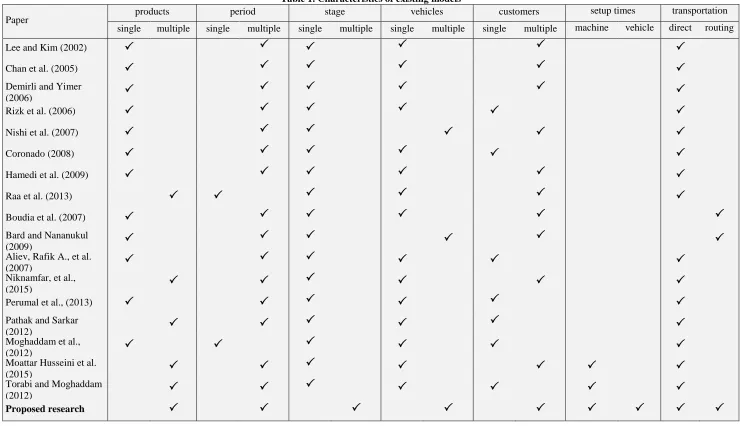
Table 1 shows a comparison among previous literature and present work at a glance. As can be seen, one of the major shortcomings in all of the above studies is that they just consider direct shipment of products to customers in generating distribution plan, and then discard vehicle routing aspects. The author could find very few papers such as Boudia et al. (2007) and Bard and Nananukul (2009) that considered production and routing decisions simultaneously. Not only the literature dealing with joint production planning and routing is very scarce, but also they just considered simplified models with single-product, single-vehicle and single-stage. Hence, to overcome these shortcomings, we will present a generalized production and distribution in current paper and formulate it as mixed integer linear programming problems. There are many successful applications of mathematical programming formulation for addressing scheduling problems in literature (e.g., Wong et al., 2012; Karimi-Nasab and Fatemi Ghomi, 2012; Ma et al. 2013; Wong et al., 2014).
Table 1. Characteristics of existing models
Paper products period stage vehicles customers
setup times transportation
single multiple single multiple single multiple single multiple single multiple machine vehicle direct routing
Lee and Kim (2002)
Chan et al. (2005)
Demirli and Yimer
(2006)
Rizk et al. (2006)
Nishi et al. (2007)
Coronado (2008)
Hamedi et al. (2009)
Raa et al. (2013)
Boudia et al. (2007)
Bard and Nananukul
(2009)
Aliev, Rafik A., et al.
(2007)
Niknamfar, et al.,
(2015)
Perumal et al., (2013)
Pathak and Sarkar
(2012)
Moghaddam et al.,
(2012)
Moattar Husseini et al.
(2015)
Torabi and Moghaddam
(2012)
2. Scope of APDP problem
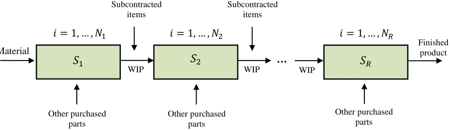
In this section, the Aggregate Production-Distribution Planning (APDP) problem suggested in current paper will be described. This problem is relevant to integration between production planning and vehicle transportation with multi-stage, multi-product and multi-vehicle systems in a two-echelon supply chain. The production part of our APDP is an extended version of classical APP problem with several machines and setup decisions. A manufacturer seeks a cost effective production level, inventory level, backorder level, and overtime and subcontract productions. It is also interested to find best workforce level including number of hired and laid-off workers. In addition, each product has a setup on machines. At each stage of production system, a number of products received from last stage and some other purchased parts are assembled to establish one unit of a product in current stage. The production system in our APDP is depicted in Figure 1.
Figure 1. Production stages within a specific time period
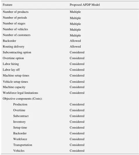
After last stage is completed, finished product is transported to customers by vehicles. A maximum number of vehicles, with limited capacities, are available to transport products from manufacturer to customers. In addition to direct shipment, vehicles can moved through a route in order to deliver products to more than one customer during a trip. It is also assumed that each vehicle is responsible for satisfying demand of all customers on route. A route is a sequence of customers in which a vehicle delivers product from a single manufacturer to multiple customers. A customer should be visited before its due date time. The route time of a vehicle is the sum of total traveling time and service time taken to visit on-route customers. The main characteristics of proposed problem are given in Table 2.
Material
𝑆1 𝑆2
…
𝑆𝑅𝑖 = 1, … , 𝑁1 𝑖 = 1, … , 𝑁2 𝑖 = 1, … , 𝑁𝑅
Other purchased parts
Other purchased parts
Other purchased parts Subcontracted
items
Subcontracted items
WIP WIP
Finished product
Table 2. Main characteristics of proposed APDP problem
Feature Proposed APDP Model
Number of products Multiple
Number of periods Multiple
Number of stages Multiple
Number of vehicles Multiple
Number of customers Multiple
Backorder Allowed
Routing delivery Allowed
Subcontracting option Considered
Overtime option Considered
Labor hiring Considered
Labor lay off Considered
Machine setup times Considered
Vehicle setup times Considered
Machine capacity Considered
Workforce legal limitations Considered
Objective components (Costs):
Production Considered
Overtime Considered
Subcontract Considered
Inventory Considered
Setup time Considered
Backorder Considered
Workforce Considered
Transportation Considered
Vehicles Considered
3. MILP formulation
which manufacturer makes direct shipments to each customer and routing decision is not incorporated. Next, we investigate second Scenario in which vehicles move through a route to deliver products to more than one customer. The parameters and variables are summarized below.
Problem parameters
𝑖, 𝑗 Index of product type 𝑖, 𝑗 = 1, … , 𝑁𝑘
𝑘 Index of production stage 𝑘 = 1, … , 𝑅
𝑡 Index of time period 𝑡 = 1, … , 𝑇
𝑚 Index of machine 𝑚 = 1, … , 𝑀
𝑞 Index of part type required for producing products 𝑞 = 1, … , 𝑄
𝑛, 𝑐, 𝑑, 𝑒 Index of customers 𝑛, 𝑐, 𝑑, 𝑒 = 1, … , 𝑁
𝜉 Index of routs and associated vehicles 𝜉 = 1, … , 𝐸
𝐶𝑉 Maximum capacity of each vehicle
𝜛 Vehicle setup time factor
𝜃𝑛 Service time of customer 𝑛
𝑑𝑢𝑛𝑡 Preferred due date of customer 𝑛 at period 𝑡
𝑡𝑐𝑑 Travel time between customers 𝑐 and 𝑑
𝜌𝜉𝑡 Vehicle setup time associated with route 𝜉 at period 𝑡
𝐷𝑖𝑡𝑛 Demand of customer 𝑛 for product type 𝑖 at period 𝑡
𝑇𝐶𝑣 Transportation cost of vehicle 𝑣 (Scenario I)
𝑇𝐶𝜉 Transportation cost of vehicle associated with route 𝜉 (Scenario II)
𝐹𝐶𝜉 Fixed cost of vehicle associated with route 𝜉
𝑀𝑇𝑇 Maximum travel time allowed for each vehicle (units of time at each period)
𝑓 Working hours of a worker at each stage of each period
𝑜𝑖𝑡𝑘 Over time production cost of product type 𝑖 in stage 𝑘 of period 𝑡
𝑐𝑖𝑡𝑘 Subcontracting cost of product type 𝑖 in stage 𝑘 of period 𝑡
ℎ𝑖𝑡𝑘 Inventory cost of product type 𝑖 at end of stage 𝑘 in period 𝑡
𝑏𝑖𝑡𝑘 Backorder cost of product type 𝑖 in stage 𝑘 of period 𝑡
𝑤𝑠𝑡𝑘 Salary cost of a worker in stage 𝑘 of period 𝑡
𝑤𝑡𝑡𝑘 Cost to hire one worker in stage 𝑘 of period 𝑡
𝑤𝑙𝑡𝑘 Cost to lay off one worker in stage 𝑘 of period 𝑡
𝐻𝑡𝑘𝑚𝑎𝑥 The maximum workforce level available for hiring in stage 𝑘 of period 𝑡
𝑊𝑡𝑘𝑚𝑎𝑥 The maximum overall workforce level in stage 𝑘 of period 𝑡
𝑊𝑡𝑚𝑎𝑥 The maximum overall workforce level in period 𝑡
𝐿𝑚𝑎𝑥 The maximum workforce level can be laid off during 𝜇 periods
𝑟𝑖𝑡𝑚𝑘 The setup cost of product type 𝑖 on machine 𝑚 in stage 𝑘 of period 𝑡
𝐴𝑖𝑗𝑘 Number of product type 𝑖 in stage 𝑘 that is needed for producing one unite of product type 𝑗 in stage 𝑘 + 1
𝜎𝑖𝑘𝑞 Number of other purchased part type 𝑞 that is needed for producing one unite of product
type 𝑖 in stage 𝑘
𝑈𝑡𝑘𝑞 Maximum available number of part type 𝑞 in stage 𝑘 of period 𝑡
𝑑𝑖𝑚𝑘 Capacity of machine 𝑚 that is needed for producing one unit of product type 𝑖 in stage 𝑘
𝑓𝑖𝑚𝑘 Capacity of machine 𝑚 that is used for setting up in producing one unit of product type 𝑖 in
stage 𝑘
𝐶𝑎𝑚𝑡𝑘 Total available capacity of machine 𝑚 in regular time of stage 𝑘 in period 𝑡
𝐶𝑡𝑘𝑚𝑎𝑥 Maximum number of products which can be subcontracted in stage 𝑘 of period 𝑡
𝛿𝑖𝑘𝑠𝑝𝑎𝑐𝑒 Amount of warehouse space occupied by one unit of product type 𝑖 at end of stage 𝑘
𝑃𝑡𝑘𝑠𝑝𝑎𝑐𝑒 Maximum warehouse space that is available after stage 𝑘 in period 𝑡
𝑒𝑖𝑡𝑘 Worker hours required per unit of product type 𝑖 in stage 𝑘 of period 𝑡
𝛾𝑡𝑘 The ratio of regular time working hours of a worker available for use in over time in stage 𝑘
of period 𝑡
𝐵𝑖𝑔𝑀 An arbitrary big positive number
Problem variables
𝑃𝑖𝑡𝑘 Units of product type 𝑖 produced in regular time of stage 𝑘 in period 𝑡
𝑂𝑖𝑡𝑘 Units of product type 𝑖 produced in over time of stage 𝑘 in period 𝑡
𝐶𝑖𝑡𝑘 Units of product type 𝑖 subcontracted in stage 𝑘 of period 𝑡
𝐼𝑖𝑡𝑘 The inventory level of product type 𝑖 at end of stage 𝑘 in period 𝑡 (WIP)
𝐵𝑖𝑡𝑘 The backorder level of product type 𝑖 in stage 𝑘 of period 𝑡
𝑊𝑡𝑘 The overall workforce level in stage 𝑘 of period 𝑡
𝐻𝑡𝑘 The number of workers hired in stage 𝑘 of period 𝑡
𝐿𝑘𝑡 The number of workers laid off in stage 𝑘 of period 𝑡
𝑌𝑖𝑡𝑚𝑘 A binary variable that indicates setup decision of product type 𝑖 on machine 𝑚 in stage 𝑘 of
period 𝑡
𝑋𝑣𝑐𝑡 A binary variable that indicates whether vehicle 𝑣 is allocated to customer 𝑐 at period 𝑡
(Scenario I)
𝑡𝑐𝑣𝑡 Start time of service at customer 𝑐 by vehicle 𝑣 in period 𝑡 (Scenario I)
𝑋𝑐𝑑𝜉𝑡 A binary variable that indicates whether (𝑐, 𝑑) is in route 𝜉 at period 𝑡 (Scenario II)
𝑡𝑐𝜉𝑡 Start time of service at customer 𝑐 in route 𝜉 of period 𝑡 (Scenario II)
𝑡0𝜉𝑡 Start time of route 𝜉 at period 𝑡 (Scenario II)
𝑉𝜉𝑡 A binary variable that indicates whether vehicle associated with route 𝜉 is selected at period 𝑡
(Scenario II)
3.1. Scenario I: APDP with Direct Shipment
The mixed integer linear programming (MILP) model for Scenario I of suggested APDP problem, called 𝑷𝟏, is presented in this section. The objective function seeks to minimize total cost of production and transportation. At first we define the parts of production cost. The costs of regular time production, overtime production and subcontracting for all product types is as presented below.
∑ ∑ ∑(𝑝𝑖𝑡𝑘𝑃
𝑖𝑡𝑘+ 𝑜𝑖𝑡𝑘𝑂𝑖𝑡𝑘 + 𝑐𝑖𝑡𝑘𝐶𝑖𝑡𝑘) 𝑇
𝑡=1 𝑁𝑘
𝑖=1 𝑅
𝑘=1
(1)
The total inventory cost including work-in-process (WIP) inventory and finished product inventory costs is formulated as follows.
∑ ∑ ∑(ℎ𝑖𝑡𝑘𝐼
𝑖𝑡𝑘) 𝑇
𝑡=1 𝑁𝑘
𝑖=1 𝑅
𝑘=1
(2)
The setup costs for all product types on associated machines are formulated in following way.
∑ ∑ ∑ ∑(𝑟𝑖𝑡𝑚𝑘𝑌
𝑖𝑡𝑚𝑘) 𝑇
𝑡=1 𝑁𝑘
𝑖=1 𝑀
𝑚=1 𝑅
𝑘=1
(3)
Since real demand of customers is related to finished products in last stage, backorder quantity is associated to 𝑅th stage of period. Therefore backorder cost is expressed as follows.
∑ ∑(𝑏𝑖𝑡𝑅𝐵 𝑖𝑡𝑅) 𝑇
𝑡=1 𝑁𝑅
𝑖=1
(4)
∑ ∑(𝑤𝑠𝑡𝑘𝑊 𝑡𝑘) 𝑅 𝑘=1 𝑇 𝑡=1 + ∑ ∑(𝑤𝑡𝑡𝑘𝐻 𝑡𝑘) 𝑅 𝑘=1 𝑇 𝑡=1 + ∑ ∑(𝑤𝑙𝑡𝑘 𝐿 𝑡 𝑘) 𝑅 𝑘=1 𝑇 𝑡=1 (5)
Regarding production costs presented in (1)-(5), total production cost (TPC) is expressed as follows.
𝑇𝑃𝐶 = ∑ ∑ ∑(𝑝𝑖𝑡𝑘𝑃𝑖𝑡𝑘+ 𝑜𝑖𝑡𝑘𝑂𝑖𝑡𝑘 + 𝑐𝑖𝑡𝑘𝐶𝑖𝑡𝑘) 𝑇 𝑡=1 𝑁𝑘 𝑖=1 𝑅 𝑘=1 + ∑ ∑ ∑(ℎ𝑖𝑡𝑘𝐼𝑖𝑡𝑘) 𝑇 𝑡=1 𝑁𝑘 𝑖=1 𝑅 𝑘=1 + ∑ ∑ ∑ ∑(𝑟𝑖𝑡𝑚𝑘𝑌 𝑖𝑡𝑚𝑘) 𝑇 𝑡=1 𝑁𝑘 𝑖=1 𝑀 𝑚=1 𝑅 𝑘=1 + ∑ ∑(𝑏𝑖𝑡𝑅𝐵 𝑖𝑡𝑅) 𝑇 𝑡=1 𝑁𝑅 𝑖=1 + ∑ ∑(𝑤𝑠𝑡𝑘𝑊𝑡𝑘) 𝑅 𝑘=1 𝑇 𝑡=1 + ∑ ∑(𝑤𝑡𝑡𝑘𝐻𝑡𝑘) 𝑅 𝑘=1 𝑇 𝑡=1 + ∑ ∑(𝑤𝑙𝑡𝑘 𝐿𝑘𝑡) 𝑅 𝑘=1 𝑇 𝑡=1 (6)
We next define direct shipment transportation costs. The transportation cost which is associated to total transportation among customers and manufacturer can be formulated as follows.
∑ (𝑇𝐶𝑣∑ ∑(𝑡0𝑐+ 𝑡𝑐0)𝑋𝑣𝑐𝑡 𝑁 𝑐=1 𝐸 𝑣=1 ) 𝑇 𝑡=1 (7)
Here 𝑡0𝑐 and 𝑡𝑐0 represents transportation time from manufacturer to customer 𝑐 and vice versa. Another important component of transportation cost is related to fixed cost of vehicles. Since number of vehicles is assumed to be determined in model, variable 𝑉𝑣𝑡 is defined to delineate whether corresponding vehicle is selected or not. Therefore total cost of vehicles, at all periods, is defined as follows.
∑ ∑(𝐹𝐶𝑣 𝑉𝑣𝑡) 𝐸 𝑣=1 𝑇 𝑡=1 (8)
Therefore, total transportation cost (TTC) incurred in Scenario I can be expressed as follows.
𝑇𝑇𝐶 = ∑ (𝑇𝐶𝑣∑ ∑(𝑡0𝑐+ 𝑡𝑐0)𝑋𝑣𝑐𝑡 𝑁 𝑐=1 𝐸 𝑣=1 ) 𝑇 𝑡=1 + ∑ ∑(𝐹𝐶𝑣 𝑉𝑣𝑡) 𝐸 𝑣=1 𝑇 𝑡=1 (9)
𝑃𝑖𝑡𝑅 + 𝑂
𝑖𝑡𝑅 + 𝐶𝑖𝑡𝑅 + 𝐵𝑖𝑡𝑅− 𝐵𝑖(𝑡−1)𝑅 + 𝐼𝑖(𝑡−1)𝑅 − 𝐼𝑖𝑡𝑅 = ∑ 𝐷𝑖𝑡𝑛 𝑁
𝑛=1 𝑖 = 1, … , 𝑁𝑅, 𝑡 = 1, … , 𝑇
(10)
The constraint set (10) ensures that total amount of finished products (last stage 𝑅) including regular time and overtime production, subcontracting, and inventory level be equal to sum of total demand of product from all customers at current period and backorders from previous periods.
𝑃𝑖𝑡𝑘+ 𝑂𝑖𝑡𝑘 + 𝐶𝑖𝑡𝑘+ 𝐼𝑖(𝑡−1)𝑘 − 𝐼𝑖𝑡𝑘 = ∑ 𝐴𝑘𝑖𝑗 𝑁𝑘+1
𝑗=1
(𝑃𝑗𝑡𝑘+1+ 𝑂𝑗𝑡𝑘+1)
𝑖 = 1, … , 𝑁𝑘, 𝑘 = 1, … , 𝑅 − 1 , 𝑡 = 1, … , 𝑇
(11)
The constraint set (11) is associated with requirement of production at each stage. It ensures an enough number of product type 𝑖 in stage 𝑘 needed for producing all products in stage 𝑘 + 1.
∑ 𝜎𝑖𝑘𝑞(𝑃𝑖𝑡𝑘+ 𝑂 𝑖𝑡𝑘) 𝑁𝑘
𝑖=1
≤ 𝑈𝑡𝑘𝑞 , 𝑘 = 1, … , 𝑅 , 𝑡 = 1, … , 𝑇 , 𝑞 = 1, … , 𝑄 (12)
The constraint set (12) indicates market limitation of parts required at each stage of periods.
∑ 𝐶𝑖𝑡𝑘 𝑁𝑘
𝑖=1
≤ 𝐶𝑡𝑘𝑚𝑎𝑥 , 𝑘 = 1, … , 𝑅 , 𝑡 = 1, … , 𝑇 (13)
∑(𝛿𝑖𝑘𝑠𝑝𝑎𝑐𝑒𝐼𝑖𝑡𝑘) 𝑁𝑘
𝑖=1
≤ 𝑃𝑡𝑘𝑠𝑝𝑎𝑐𝑒 , 𝑘 = 1, … , 𝑅 , 𝑡 = 1, … , 𝑇 (14)
The constraint sets (13) and (14) express quantities of subcontracting and required shortage space should not exceed maximum number of products which can be subcontracted and maximum warehouse space available, respectively.
𝑃𝑖𝑡𝑘+ 𝑂
𝑖𝑡𝑘 ≤ 𝐵𝑖𝑔𝑀 ∑ 𝑌𝑖𝑡𝑚𝑘 𝑀
𝑚=1
, 𝑖 = 1, … , 𝑁𝑘 , 𝑘 = 1, … , 𝑅 , 𝑡 = 1, … , 𝑇 (15)
∑(𝑑𝑖𝑚𝑘 𝑃
𝑖𝑡𝑘+ 𝑓𝑖𝑚𝑘 𝑌𝑖𝑡𝑘) 𝑁𝑘
𝑖=1
≤ 𝐶𝑎𝑚𝑡𝑘 , 𝑚 = 1, … , 𝑀 ,
𝑘 = 1, … , 𝑅 , 𝑡 = 1, … , 𝑇
(16)
∑(𝑑𝑖𝑚𝑘 𝑂𝑖𝑡𝑘) 𝑁𝑘
𝑖=1
≤ 𝛽𝑚𝑡𝑘 𝐶𝑎𝑚𝑡𝑘 , 𝑚 = 1, … , 𝑀 ,
𝑘 = 1, … , 𝑅 , 𝑡 = 1, … , 𝑇
(17)
The constraint sets (16) and (17) indicate machine capacity. Constraint (16) ensures that sum of processing times and setup times on a specific machine should not be greater than its regular time capacity, and constraint (17) ensures that processing time of overtime production does not violate machine overtime capacity.
𝑊𝑡𝑘 = 𝑊
𝑡−1𝑘 + 𝐻𝑡𝑘− 𝐿𝑘𝑡 , 𝑘 = 1, … , 𝑅 , 𝑡 = 1, … , 𝑇 (18)
∑(𝑒𝑖𝑡𝑘𝑃𝑖𝑡𝑘) 𝑁𝑘
𝑖=1
≤ 𝑓𝑊𝑡𝑘 , 𝑘 = 1, … , 𝑅 , 𝑡 = 1, … , 𝑇 (19)
∑(𝑒𝑖𝑡𝑘𝑂 𝑖𝑡𝑘) 𝑁𝑘
𝑖=1
≤ 𝑓𝛾𝑡𝑘𝑊
𝑡𝑘 , 𝑘 = 1, … , 𝑅 , 𝑡 = 1, … , 𝑇 (20)
𝑊𝑡𝑘 ≤ 𝑊
𝑡𝑘𝑚𝑎𝑥 , 𝑘 = 1, … , 𝑅 , 𝑡 = 1, … , 𝑇 (21)
𝐻𝑡𝑘 ≤ 𝐻
𝑡𝑘𝑚𝑎𝑥 , 𝑘 = 1, … , 𝑅 , 𝑡 = 1, … , 𝑇 (22)
∑ 𝑊𝑡𝑘 𝑅
𝑘=1
≤ 𝑊𝑡𝑚𝑎𝑥 , 𝑡 = 1, … , 𝑇 (23)
∑ ∑ 𝐿𝜆𝑘
𝑅
𝑘=1 𝜆+𝜇
𝑡=𝜆
≤ 𝐿𝑚𝑎𝑥 , 𝜆 = 1, … , 𝑇 − 𝜇 (24)
working hours in regular time and overtime. They guarantee that amount of hours required for production in regular time and overtime should not exceed maximum working hours available, respectively. The constraint set (21) restricts overall workforce level to be less than a maximum threshold, while constraint set (22) ensures that hired workforce for each stage in each period should do not exceed maximum workforce level available. The constraint set (23) presents limitation of total workforce level in each period. The constraint (24) indicates legal limitation to laying off workers during 𝜇 periods. The total number of workers laid off should not exceed a legal threshold.
∑ 𝑋𝑣𝑐𝑡 𝐸
𝑣=1
= 1 , 𝑐 = 1, … , 𝑁 , 𝑡 = 1, … , 𝑇 (25)
∑ 𝑋𝑣𝑐𝑡 𝑁
𝑐=1
= 1 , 𝑣 = 1, … , 𝐸 , 𝑡 = 1, … , 𝑇 (26)
The constraint set (25) ensures that demand of each customer should be satisfied at each period, and constraint set (26) enforces that each vehicle is assigned to exactly one customer.
∑ 𝐷𝑖𝑡𝑐𝑋𝑣𝑐𝑡 𝑁
𝑖=1
≤ 𝐶𝑉 , 𝑐 = 1, … , 𝑁 , 𝑡 = 1, … , 𝑇 , 𝑣 = 1, … , 𝐸 (27)
The constraint set (27) guarantees that total demand of a customer satisfied by vehicle allocated to that customer should not exceed vehicle capacity.
𝑡𝑐𝑣𝑡 ≤ 𝑑𝑢
𝑐𝑡 𝑋𝑣𝑐𝑡 , 𝑐 = 1, … , 𝑁 , 𝑣 = 1, … , 𝐸 , 𝑡 = 1, … , 𝑇 (28)
The constraint set (28) enforces vehicles to start service of customers before due date.
𝑡𝑐𝑣𝑡 ≥ (𝜌𝑣𝑡+ 𝑡0𝑐)𝑋𝑣𝑐𝑡 , 𝑐 = 1, … , 𝑁 , 𝑣 = 1, … , 𝐸 , 𝑡 = 1, … , 𝑇 (29)
In order to consider setup operation of vehicles, start time of customer service should be greater than sum of vehicle setup time and transportation time between manufacturer and customer. This constraint is indicated by Eq. (29).
𝜌𝑣𝑡 = 𝜛 ∑ 𝜃
𝑐𝑋𝑣𝑐𝑡 𝑁
𝑐=1
, 𝑣 = 1, … , 𝐸 , 𝑡 = 1, … , 𝑇 (30)
∑ 𝑋𝑣𝑐𝑡 𝑁
𝑐=1
≤ 𝑉𝑣𝑡 , 𝑣 = 1, … , 𝐸 , 𝑡 = 1, … , 𝑇 (31)
The constraint (31) indicates whether a vehicle is employed in a period. If one of customers is allocated to vehicle 𝑣, vehicle 𝑣 is employed (𝑉𝑣𝑡 = 1). Otherwise, we have 𝑉𝑣𝑡 = 0.
∑(𝑋𝑣𝑐𝑡 (𝑡
0𝑐+ 𝑡𝑐0)) 𝑁
𝑐=1
≤ 𝑀𝑇𝑇 , 𝑣 = 1, … , 𝐸 , 𝑡 = 1, … , 𝑇 (32)
The maximum travel time allowed for each vehicle is ensured by constraint set (32).
𝑃𝑖𝑡𝑘 ≥ 0, 𝑂
𝑖𝑡𝑘 ≥ 0, 𝐶𝑖𝑡𝑘 ≥ 0, 𝐼𝑖𝑡𝑘 ≥ 0, 𝐵𝑖𝑡𝑘 ≥ 0, 𝑊𝑡𝑘 ≥ 0, 𝐻
𝑡𝑘 ≥ 0, 𝐿𝑘𝑡 ≥ 0 , 𝑡𝑐𝑣𝑡 ≥ 0, 𝑌𝑖𝑡𝑚𝑘= (0,1), 𝑋
𝑐𝑣𝑡 = (0,1), 𝑉𝑣𝑡= (0,1)
(33)
𝑖 = 1, … , 𝑁𝑘, 𝑡 = 1, … , 𝑇, 𝑘 = 1, … , 𝑅 , 𝑚 = 1, … , 𝑀 𝑣 = 1, … , 𝐸 , 𝑐 = 0, … , 𝑁 + 1, 𝑑 = 0, … , 𝑁 + 1
Finally, binary and non-negativity natures of variables are indicated by constraints in Eq. (33).
3.2. Scenario II: APDP with Routing
The mixed-integer linear programming (MILP) model for Scenario II of suggested APDP problem, called 𝑷𝟐, will be presented in this section. As mentioned before, vehicles can move through a route to deliver products to more than one customer in Scenario II. Therefore, production part of Scenarios I and II is identical, and transportation part should be revised. The transportation issue is appeared in two sections of mathematical formulation, i.e., (i) second term of objective function (TTC), and (ii) transportation related constraints. In sequel, we define routing costs considered in objective function.
The first component of routing cost is total cost of transportation carried out from manufacturer to customers. This transportation cost which is associated to total transportation time and distance among manufacturer and customers on selected routes can be formulated as follows.
∑ ∑ (𝑇𝐶𝜉 ∑ ∑ (𝑡𝑐𝑑𝑋𝑐𝑑𝜉𝑡) 𝑁+1
𝑑=0 𝑁+1
𝑐=0
) 𝐸
𝜉=1 𝑇
𝑡=1
(34)
∑ ∑(𝐹𝐶𝜉 𝑉𝜉𝑡) 𝐸 𝜉=1 𝑇 𝑡=1 (35)
Hence, total transportation cost (TTC) considered in Scenario II is expressed as follows.
𝑇𝑇𝐶 = ∑ ∑ (𝑇𝐶𝜉∑ ∑ (𝑡𝑐𝑑𝑋𝑐𝑑𝜉𝑡) 𝑁+1 𝑑=0 𝑁+1 𝑐=0 ) 𝐸 𝜉=1 𝑇 𝑡=1 + ∑ ∑(𝐹𝐶𝜉 𝑉𝜉𝑡) 𝐸 𝜉=1 𝑇 𝑡=1 (36)
Here we formulate transportation related constraints in Scenario II. According to definition of two different Scenarios, the objective function and all the constraints presented in Eq.s (10)-(24) are identical in both Scenarios. The transportation related constraints for Scenario II are as follows.
∑ 𝑋𝑐𝑑𝜉𝑡 𝑁+1
𝑑=0
= 𝑍𝑐𝜉𝑡 , 𝑐 = 1, … , 𝑁 , 𝜉 = 1, … , 𝐸 , 𝑡 = 1, … , 𝑇 (37)
∑ 𝑍𝑐𝜉𝑡 𝐸
𝜉=1
= 1 , 𝑐 = 1, … , 𝑁 , 𝑡 = 1, … , 𝑇 (38)
∑ 𝑋𝑐𝑒𝜉𝑡 𝑁+1 𝑐=0 − ∑ 𝑋𝑒𝑑𝜉𝑡 𝑁+1 𝑑=0
= 0, 𝑒 = 1, … , 𝑁 , 𝜉 = 1, … , 𝐸 , 𝑡 = 1, … , 𝑇 (39)
∑ 𝑋0𝑑𝜉𝑡 𝑁+1
𝑑=1
= 1 , 𝜉 = 1, … , 𝐸 , 𝑡 = 1, … , 𝑇 (40)
∑ 𝑋𝑐(𝑁+1)𝜉𝑡 𝑁
𝑐=1
= 1 , 𝜉 = 1, … , 𝐸 , 𝑡 = 1, … , 𝑇 (41)
∑ ∑ (𝐷𝑖𝑡𝑛𝑍𝑛𝜉𝑡) 𝑁𝑅
𝑖=1 𝑁
𝑛=1
≤ 𝐶𝑉 , 𝜉 = 1, … , 𝐸 , 𝑡 = 1, … , 𝑇 (42)
𝑡𝑐𝜉𝑡 + 𝜃𝑐 + 𝑡𝑐𝑑 ≤ 𝑡𝑑𝜉𝑡+ 𝐵𝑖𝑔𝑀 (1 − 𝑋𝑐𝑑𝜉𝑡) , 𝑐 = 0, … , 𝑁 + 1
𝑡𝑐𝜉𝑡 ≤ 𝑑𝑢𝑐𝑡 𝑍𝑐𝜉𝑡 , 𝑐 = 1, … , 𝑁 , 𝜉 = 1, … , 𝐸 , 𝑡 = 1, … , 𝑇 (44)
𝑡0𝜉𝑡 ≥ 𝜌𝜉𝑡 , 𝜉 = 1, … , 𝐸 , 𝑡 = 1, … , 𝑇 (45)
𝜌𝜉𝑡 = 𝜛 ∑ 𝜃
𝑐𝑍𝑐𝜉𝑡 𝑁
𝑐=1
, 𝜉 = 1, … , 𝐸 , 𝑡 = 1, … , 𝑇 (46)
∑ 𝑍𝑐𝜉𝑡 𝑁
𝑐=1
≤ 𝑁 𝑉𝜉𝑡 , 𝜉 = 1, … , 𝐸 , 𝑡 = 1, … , 𝑇 (47)
∑ ∑ (𝑡𝑐𝑑𝑋𝑐𝑑𝜉𝑡) 𝑁+1
𝑑=0 𝑁+1
𝑐=0
≤ 𝑀𝑇𝑇 , 𝜉 = 1, … , 𝐸 , 𝑡 = 1, … , 𝑇 (48)
The constraint sets (37)-(48) are relevant to routing decisions in transportation of products from manufacturer to customers and substitute instead of Eq.s (25)-(32) in Scenario I to establish Scenario II. The constraint (37) defines relation between customer assignment variables 𝑋𝑐𝑑𝜉𝑡 and 𝑍𝑐𝜉𝑡. The constraint (38) ensures that each customer should be visited exactly once. Constraint (39) enforces each customer to be visited after and before other unique customers on a specific route. The constraints (40) and (41) define first and last customer on routes. The constraint (42) guarantees that total demand on a route should not violate vehicle capacity. The feasibility of vehicle schedules is ensured by constraints (43). The constraint (44) guarantees that customer demand should be met before due date. The constraint (45) restricts route start time to be greater than vehicle setup time. Constraint (46) calculates vehicle setup time. The constraint (47) indicates whether a vehicle is employed in a period or not. If at least one customer is selected for a specific route 𝜉 in each period 𝑡 (∑𝑁𝑐=1𝑍𝑐𝜉𝑡 ≥ 1), vehicle should be employed in that period (𝑉𝜉𝑡 = 1). The constraint (48) ensures a maximum travel time is allowed for each vehicle. The variables 𝑡𝑐𝜉𝑡 and 𝑡0𝜉𝑡 are non-negative, and
variables 𝑋𝑐𝑑𝜉𝑡, 𝑍𝑐𝜉𝑡 and 𝑉𝜉𝑡 are binary.
4. Numerical analysis
In previous section, proposed APDP problem was formulated as MILP models for two different Scenarios. In sequel, we investigate performance of formulations. For this purpose, a numerical example with following structure has been considered:
Number of product types: 4
Number of time periods: 5
Number of stages at each period: 3
Number of machines at each stage: 3
Number of required parts: 3
The total demand of customers is given in Table 3. Tables 4-6 show unit cost of production, holding/backorder and workers respectively.
Table 3. Information on customer demand
Customer Product
Period
𝑡 = 1 𝑡 = 2 𝑡 = 3 𝑡 = 4 𝑡 = 5
𝑐 = 1 𝑖 = 1 50 200 150 250 400
𝑖 = 2 350 750 150 350 550
𝑖 = 3 400 850 50 150 750
𝑖 = 4 200 300 450 500 300
𝑖 = 5 100 350 250 400 200
𝑐 = 2 𝑖 = 1 300 350 200 450 250
𝑖 = 2 850 600 400 650 900
𝑖 = 3 200 50 150 300 200
𝑖 = 4 850 400 600 750 450
𝑖 = 5 350 400 500 450 350
𝑐 = 3 𝑖 = 1 200 150 50 400 200
𝑖 = 2 650 700 400 550 250
𝑖 = 3 450 400 650 850 950
𝑖 = 4 50 250 300 250 400
𝑖 = 5 650 150 200 250 350
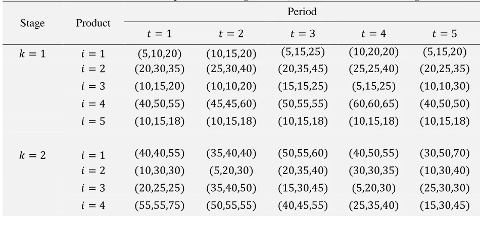
Table 4. The unit costs of production in regular time, over time and subcontracting
Stage Product
Period
𝑡 = 1 𝑡 = 2 𝑡 = 3 𝑡 = 4 𝑡 = 5
𝑘 = 1 𝑖 = 1 (5,10,20) (10,15,20) (5,15,25) (10,20,20) (5,15,20)
𝑖 = 2 (20,30,35) (25,30,40) (20,35,45) (25,25,40) (20,25,35)
𝑖 = 3 (10,15,20) (10,10,20) (15,15,25) (5,15,25) (10,10,30)
𝑖 = 4 (40,50,55) (45,45,60) (50,55,55) (60,60,65) (40,50,50)
𝑖 = 5 (10,15,18) (10,15,18) (10,15,18) (10,15,18) (10,15,18)
𝑘 = 2 𝑖 = 1 (40,40,55) (35,40,40) (50,55,60) (40,50,55) (30,50,70)
𝑖 = 2 (10,30,30) (5,20,30) (20,35,40) (30,30,35) (10,30,40)
Stage Product
Period
𝑡 = 1 𝑡 = 2 𝑡 = 3 𝑡 = 4 𝑡 = 5
𝑖 = 5 (30,40,55) (25,30,45) (35,45,50) (30,40,55) (20,25,35)
𝑘 = 3 𝑖 = 1 (60,70,85) (30,45,55) (55,75,80) (35,50,60) (40,55,65)
𝑖 = 2 (10,20,25) (40,50,55) (25,30,35) (15,30,40) (35,55,65)
𝑖 = 3 (25,30,40) (50,55,55) (20,45,50) (20,30,45) (10,15,15)
𝑖 = 4 (30,40,40) (25,25,45) (35,45,60) (55,65,65) (45,50,50)
𝑖 = 5 (45,55,55) (25,35,50) (20,30,45) (35,45,50) (25,35,50)
Table 5. The unit costs of holding and backorder (𝒉, 𝒃)
Customer Product
Period
𝑡 = 1 𝑡 = 2 𝑡 = 3 𝑡 = 4 𝑡 = 5
𝑐 = 1 𝑖 = 1 (10,15) (5,20) (10,5) (25,15) (5,5)
𝑖 = 2 (15,25) (5,10) (10,10) (20,10) (10,25)
𝑖 = 3 (30,20) (20,10) (15,5) (25,10) (10,25)
𝑖 = 4 (25,30) (5,20) (20,30) (15,5) (25,20)
𝑖 = 5 (20,30) (5,15) (20,10) (15,25) (15,10)
𝑐 = 2 𝑖 = 1 (5,20) (25,10) (15,30) (20,10) (5,15)
𝑖 = 2 (10,20) (25,5) (15,10) (15,5) (5,25)
𝑖 = 3 (15,10) (20,10) (25,5) (30,10) (5,5)
𝑖 = 4 (20,10) (30,25) (20,30) (10,30) (10,10)
𝑖 = 5 (25,25) (10,20) (30,15) (20,20) (15,30)
𝑐 = 3 𝑖 = 1 (25,20) (15,10) (25,10) (15,30) (5,30)
𝑖 = 2 (20,5) (15,15) (5,10) (20,15) (30,30)
𝑖 = 3 (15,5) (5,20) (25,15) (5,20) (30,10)
𝑖 = 4 (5,20) (30,10) (15,15) (30,5) (10,25)
Table 6. The unit costs of worker salary (𝒘𝒔𝒕𝒌), hiring (𝒘𝒕𝒕𝒌) and lay off (𝒘𝒍𝒕𝒌)
Parameter Stage
Period
𝑡 = 1 𝑡 = 2 𝑡 = 3 𝑡 = 4 𝑡 = 5
𝑤𝑠𝑡𝑘 𝑘 = 1 1070 1210 1450 1390 1480
𝑘 = 2 1320 1020 1420 1460 1340
𝑘 = 3 1380 1370 1190 1320 1080
𝑤𝑡𝑡𝑘 𝑘 = 1 398 390 430 442 451
𝑘 = 2 356 436 432 333 324
𝑘 = 3 400 492 369 418 345
𝑤𝑙𝑡𝑘 𝑘 = 1 276 226 251 270 290
𝑘 = 2 296 255 214 215 226
𝑘 = 3 285 226 282 225 293
The transportation times among manufacturer and customers are presented in Table 7.
Table 7. Transportation times
Manufacturer Customer 𝑘 = 1 Customer 𝑘 = 2 Customer 𝑘 = 3
Manufacturer 0 150 275 225
Customer 𝑘 = 1 150 0 225 300
Customer 𝑘 = 2 225 250 0 200
Customer 𝑘 = 3 275 350 300 0
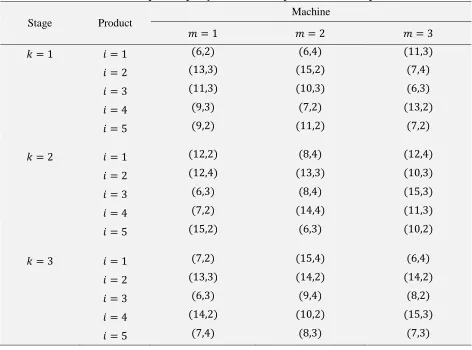
Table 8. Required capacity of machines for production and setup
Stage Product
Machine
𝑚 = 1 𝑚 = 2 𝑚 = 3
𝑘 = 1 𝑖 = 1 (6,2) (6,4) (11,3)
𝑖 = 2 (13,3) (15,2) (7,4)
𝑖 = 3 (11,3) (10,3) (6,3)
𝑖 = 4 (9,3) (7,2) (13,2)
𝑖 = 5 (9,2) (11,2) (7,2)
𝑘 = 2 𝑖 = 1 (12,2) (8,4) (12,4)
𝑖 = 2 (12,4) (13,3) (10,3)
𝑖 = 3 (6,3) (8,4) (15,3)
𝑖 = 4 (7,2) (14,4) (11,3)
𝑖 = 5 (15,2) (6,3) (10,2)
𝑘 = 3 𝑖 = 1 (7,2) (15,4) (6,4)
𝑖 = 2 (13,3) (14,2) (14,2)
𝑖 = 3 (6,3) (9,4) (8,2)
𝑖 = 4 (14,2) (10,2) (15,3)
𝑖 = 5 (7,4) (8,3) (7,3)
Table 9. Information on machines’ capacity (𝑪𝒂, 𝜷)
Stage Machine
Period
𝑡 = 1 𝑡 = 2 𝑡 = 3 𝑡 = 4 𝑡 = 5
𝑘 = 1 𝑖 = 1 (7920, 0.78) (5760, 0.80) (4450, 0.67) (5040, 0.66) (5640, 0.94)
𝑖 = 2 (6380, 0.51) (5050, 0.89) (6420, 0.91) (6850, 0.85) (4890, 0.54)
𝑖 = 3 (4470, 0.61) (5190, 0.65) (5280, 0.80) (5700, 0.56) (6040, 0.82)
𝑘 = 2 𝑖 = 1 (5230, 0.54) (6040, 0.79) (6050, 0.72) (7280, 0.85) (7180, 0.82)
𝑖 = 2 (6580, 0.91) (5520, 0.90) (7250, 0.65) (6140, 0.81) (5410, 0.58)
𝑖 = 3 (7760, 0.51) (7510, 0.83) (6210, 0.72) (6490, 0.71) (6350, 0.90)
𝑘 = 3 𝑖 = 1 (4840, 0.77) (5210, 0.78) (5890, 0.86) (4930, 0.75) (7380, 0.58)
𝑖 = 2 (4780, 0.60) (4910, 0.89) (4690, 0.51) (4920, 0.72) (5750, 0.71)
𝑖 = 3 (5250, 0.51) (7700, 0.80) (5730, 0.52) (4740, 0.53) (7620, 0.73)
The preferred due date of customers at each period is presented by Table 10.
Table 10. Customer due dates
Customer
Period
𝑡 = 1 𝑡 = 2 𝑡 = 3 𝑡 = 4 𝑡 = 5
𝑐 = 1 520 730 860 770 580
𝑐 = 2 650 690 900 570 850
𝑐 = 3 760 660 580 680 700
Two MILP models are implemented in a commercial solver LINGO 11.0. Based on the attained results, the main significant difference between two Scenarios is that direct shipping provides the benefit of eliminating intermediate warehouses, whereas routing causes lower transportation cost by shipment to multiple customers on a single vehicle and the use of routing mode results in better utilization of the vehicles. According to the results, the inventory cost of Scenario I is obtained 487652, while that of Scenario II is calculated 623902. Moreover, transportation cost incurred by Scenario I is 329113, while this value is 148294 by Scenario II.
Table 11. Structure of test problems
Class Problem Periods Stages Products Machines Customers Vehicles Parts
Small P1 5 2 2 1 5 2 2
P2 5 2 2 1 10 2 2
P3 5 2 3 2 15 2 4
P4 5 2 3 2 20 2 4
Medium P5 8 3 4 4 25 4 5
P6 8 3 4 4 30 4 5
P7 8 3 5 6 35 4 7
P8 8 3 5 6 40 4 7
Large P9 10 4 8 8 45 6 8
P10 10 4 8 8 55 6 8
P11 10 4 10 10 60 6 10
P12 10 4 10 10 80 6 10
Table 12. The computational results for Scenario I
Class Problem
Number of Variables Number of
Constraints CPU(s) Integer Continuous
Small P1 180 70 333 32
P2 230 120 458 48
P3 330 210 643 59
P4 380 260 768 106
Medium P5 1352 1184 2646 331
P6 1512 1344 3006 456
P7 1792 1840 3558 538
P8 1952 2000 3918 603
Large P9 4420 5260 8048 1205
P10 5020 5860 9348 1458
P11 5720 7600 10398 1672
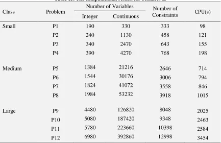
Table 13. The computational results for Scenario II
Class Problem
Number of Variables Number of
Constraints CPU(s) Integer Continuous
Small P1 190 330 333 98
P2 240 1130 458 121
P3 340 2470 643 155
P4 390 4270 768 198
Medium P5 1384 21216 2646 714
P6 1544 30176 3006 794
P7 1824 41072 3558 846
P8 1984 53232 3918 1015
Large P9 4480 126820 8048 2025
P10 5080 187420 9348 2463
P11 5780 223660 10398 2584
P12 6980 392860 12998 3454
As can be seen, total number of constraints is equal in both Scenarios and varies from 333 to 12998. It can be verify from enumeration of number of constraints in both models. In Scenario I, the total number of integer variables varies from 180 to 6920, while in Scenario II it varies from 190 to 6980. Therefore, it can be concluded that the total number of integer variables for a specific problem in Scenario II is slightly greater than that value of same problem in Scenario I. In addition, it is observed that there is a significant difference in total number of continuous variables between Scenario I and II. The minimum and maximum number of continuous variables in Scenario I is 700 and 8800, while those values of Scenario II is 330 and 392860. The increasing behavior of number of variables and constraints of Scenario I and II is depicted by Figures 2 and 3 respectively. There is obviously a high difference between two Scenarios. As indicated in Figure 3, the total number of continuous variables in Scenario II exceeds the figure limit (12000) in medium and large classes of problems.
Figure 2. Problem dimension versus problem size in Scenario I
Figure 3. Problem dimension versus problem size in Scenario II
0 1500 3000 4500 6000 7500 9000 10500 12000
Small Medium Large
Integer Variables Continuous Variables Constraints
0 1500 3000 4500 6000 7500 9000 10500 12000
Small Medium Large
Figure 4. The CPU time versus problem size
5. Conclusion
In this paper we introduced an aggregate production-distribution planning problem, consisting of two sub-problems, aggregate production planning problem and distribution planning problem in a two-echelon supply chain. The suggested APDP aims to jointly optimize production, inventory, subcontracting, and transportation decisions in order to supply and deliver demand of geographically dispersed customers while minimizing total cost of system. Unlike most of past researches, an extended version of sub-problems with multi-stage, multi-product, multi-vehicle including several shop-floor machines and setup decisions was considered. We also introduced two distinct scenarios for distribution decisions, i.e., direct shipment and routing, and formulated each one as MILP models. An illustrative numerical example and some test problems were employed and comparison results of MILP models on number of constraints, number of variables and CPU time were reported.
References
Aliev, Rafik A., et al., 2007, “Fuzzy-genetic approach to aggregate production–distribution planning in supply chain management’, Information Sciences, 177, 4241-4255.
Ashayeri J, Selen W., 2003, “A production planning model and a case study for the pharmaceutical industry in the Netherlands”, Journal of Logistics: Research and Applications, 6, 37–50.
Bard JF, Nananukul N., 2009, “The integrated production–inventory–distribution–routing problem”, Journal of Scheduling, 12, 257–80.
Boudia M, Louly MAO, Prins C., 2007, “A reactive GRASP and path relinking for a combined production– distribution problem”, Computers & Operations Research, 34, 3402–3519.
Chan FTS, Chung SH, Wadhwa S., 2005, “A hybrid genetic algorithm for production and distribution”,
Omega, 33, 345–55.
Coronado JL., 2008, “An optimization model for strategic supply chain design under stochastic capacity disruptions. Texas: College of Engineering”, Texas A&M University; 1–110.
Demirli K, Yimer AD., 2006, “Production–distribution planning with fuzzy costs. In: Proceedings of annual meeting of North American fuzzy information processing society”, (NAFIPS 2006). 702–707.
0 500 1000 1500 2000 2500 3000
Small Medium Large
Fahimnia, B., Farahani, R.Z., Marian, R. Luong, L., 2013, “A review and critique on integrated production– distribution planning models and techniques”, Journal of Manufacturing Systems, 32, 1–19.
Ghasemy Yaghin, R., Torabi, S.A., and Fatemi Ghomi S.M.T., 2012, “Integrated markdown pricing and aggregate production planning in a two echelon supply chain: A hybrid fuzzy multiple objective approach”,
Applied Mathematical Modelling, 36, 6011–6030.
Haehling LC., 1970, “Production and employment scheduling in multi-stage production systems”, Naval
Research Logistics Quarterly, 17(2), 193 –8.
Hamedi M, Farahani RZ, Husseini MM, Esmaeilian GR., 2009, “A distribution planning model for natural gas supply chain: a case study”, Energy Policy, 37, 799–812.
Holt CC, Modigliani F, Simmon HA., 1955, “A linear decision rule for production and employment scheduling”, Management Science, 2(1), 1–30.
Jain, A., and Palekar, U.S., 2005, “Aggregate production planning for a continuous reconfigurable manufacturing process”, Computers & Operations Research, 32, 1213–1236.
Jamalnia, A., and Soukhakian, M.A., 2009, “A hybrid fuzzy goal programming approach with different goal priorities to aggregate production planning”, Computers & Industrial Engineering, 56, 1474–1486.
Karimi-Nasab, M., and Fatemi Ghomi S.M.T., 2012, “Multi-objective production scheduling with controllable processing times and sequence-dependent setups for deteriorating items”, International Journal
of Production Research, 50, (24), 7378-7400.
Karmarkar, U.S., and Rajaram, K., 2012, “Aggregate production planning for process industries under oligopolistic competition”, European Journal of Operational Research, 223, 680–689.
Lee YH, Kim SH., 2002, “Production–distribution planning in supply chain considering capacity constraints”, Computers & Industrial Engineering; 43, 169–190.
Ma, H.L. Felix T.S. Chan and Chung, S.H., 2013, “Minimizing earliness and tardiness by integrating production scheduling with shipping information”, International Journal of Production Research, 51, (8), 2253-2267.Moattar Husseini, Zohre, et al., 2015, “Multi-objective integrated production distribution planning concerning manufacturing partners”, International Journal of Computer Integrated Manufacturing. 28, 1313-1330.
Moghaddam, Mohsen, Masoud Rabbani, and Babak Maleki-Shoja, 2012, “Integrating lateral transshipment to aggregate production–distribution planning considering time value of money and exchange rate” International Journal of Operational Research, 13, 439-464.
Niknamfar, Amir Hossein, Seyed Taghi Akhavan Niaki, and Seyed Hamid Reza Pasandideh, 2015, “Robust optimization approach for an aggregate production–distribution planning in a three-level supply chain”, The
International Journal of Advanced Manufacturing Technology, 76, 623-634.
Nishi T, Konishi M, Ago M., 2007, “A distributed decision-making system for integrated optimization of production scheduling and distribution for aluminum production line”, Computers & Chemical Engineering, 31:1205–1221.
Pathak, Savita, and Seema Sarkar, 2012, “A fuzzy optimization model to the aggregate production/distribution planning decision in a multi-item supply chain network”, International Journal of
Management Science and Engineering Management, 7, 163-173.
Perumal, Ashoka Varthanan, N. Murugan, and G. Mohan Kumar, 2013, “A discrete PSO approach for generating an integrated multi-plant aggregate production-distribution plan”, International Journal of
Knowledge-based and Intelligent Engineering Systems, 17, 195-207.
Raa, B. Dullaert, W., and Aghezzaf, EL-H., 2013, “A matheuristic for aggregate production–distribution planning with mould sharing”, Int. J. Production Economics, 145, 29–37.
Rizk N, Martel A, D’Amours S., 2006, “Multi-item dynamic production–distribution planning in process industries with divergent finishing stages”, Computers & Operations Research, 33, 3600–3623.
1726-Wang, R-C, and Liang, T-F., 2005, “Applying possibilistic linear programming to aggregate production planning”, Int. J. of Production Economics, 98, 328–341.
Wang, R-C, and Liang, T-F., 2004, “Application of fuzzy multi-objective linear programming to aggregate production planning”, Computers and Industrial Engineering, 46, 17–41.
Wong, C.S., Felix T.S. Chan and Chung, S.H., 2012, “A genetic algorithm approach for production scheduling with mould maintenance consideration”, International Journal of Production Research, 50, (20), 5683-5697.
Wong, C.S., Felix T.S. Chan, and Chung, S.H., 2014, “Decision-making on multi-mould maintenance in production scheduling”, International Journal of Production Research, 52, (19), 5640-5655.