Development and Application of an ALE Large
Deformation Formulation
Y. Tadi benii;M. R. Movahhedyii; and G.H. Farrahiiii
i Y. Tadi beni is Ph.D. Student in the Department of Mechanical Engineering, Sharif University of Technology, Tehran, Iran (e-mail: [email protected]
ii M. R. Movahhedy is Associate professor in the Department of Mechanical Engineering, Sharif University of Technology, Tehran, Iran (e-mail: [email protected])
iii G.H. Farrahi is Professor in the Department of Mechanical Engineering, Sharif University of Technology, Tehran, Iran (e-mail: [email protected])
ABSTRACT
This paper presents a complete derivation and implementation of the Arbitrary Lagrangian Eulerian (ALE) formulation for the simulation of nonlinear static and dynamic problems in solid mechanics. While most of the previous work done on ALE for dynamic applications was mainly based on operator split and explicit calculations, this work derives the quasi-static and dynamic ALE equations in its simple and correct form, using a fully coupled implicit approach. Full expression for the ALE virtual work equations is given. Time integration relations for the dynamic equations are also derived. Examples of quasi-static and dynamic large deformation applications are presented.
KEYWORDS
FEM, ALE, Large deformation, Coupled formulations, implicit dynamic analysis.
1. INTRODUCTION
The Arbitrary Lagrangian Eulerian (ALE) formulation has emerged in recent years as a technique that can alleviate many of the drawbacks of the traditional Lagrangian and Eulerian formulations [1-6,11]. In the ALE analysis, the finite element mesh is neither attached to the material nor fixed in space, but each degree of freedom of the system may be assigned an arbitrary motion independent of the material deformation. Therefore, ALE is a general formulation that can be reduced to Eulerian or Lagrangian formulation as special cases. By combining the merits of both the Lagrangian and Eulerian formulations, ALE can easily describe different types of boundary conditions and prevent mesh distortion. The ALE equations are derived by substituting the relationship between the material time derivative and grid time derivative into the governing equations of continuum mechanics. The various ALE procedures in the literature may be divided into two categories. In one category, an operator-split approach is used in which each step of the analysis is decoupled into a Lagrangian step and a convection step. In the former step, the solution to
Lagrangian motion is obtained, and in the latter step the solution is mapped to the desired mesh to complete the ALE step [4, 2]. In the second category, a fully coupled approach is used that represents a true kinematic description where material deformation is described relative to a moving reference configuration. While the first approach is computationally convenient, it reduces the accuracy of the analysis [2]. In fact, the operator-split approach may not be called a strictly ALE approach, since it is practically equivalent to an updated Lagrangian formulation followed by consecutive remeshing. In contrast, the fully coupled approach is a true ALE formulation, because in this approach the grid and material motion occur simultaneously.
2. DESCRIPTION OF MOTION IN THE ALE
Kinematics
In the ALE description of motion, neither the material configuration X nor the spatial configuration x is taken as the reference. Instead, a third domain, called the referential configuration χ is used. In this description, the material configuration is identified by a set of material point coordinates t mxi while the reference configuration, or grid, is identified by an independent set of grid point coordinates t gxi . Figure 1 shows the one-to-one mapping that relates the three configurations.
Figure 1: Schematic diagram of the mapping between the three domains in the ALE description
The referential domain χ is mapped into the material
and spatial domains by tx andt gx , respectively. The domain of the material points,X, is related to the spatial points, x, by
(1) ( , )
t t m i i j
x = x X t
The mapping of t gx from the referential domain to the spatial domain, which can be understood as the motion of the grid points in the spatial domain, is represented by
(2)
( , )
t t g i i j
x = x
χ
tThe material velocity tv
i, the grid point velocity tvig,
and the convective velocity tc
i at time t are given by
(3) X
v |
t m t i
i
j
x t
∂ =
∂
,
v |t g t g i
i j
x t χ
∂ =
∂
,
g
i i
v v
t t t i
c
− =
In addition, the boundaries of the material and grid configurations should coincide, i.e.
(4)
( vt tv )g t | 0
i − i ni o n th e b o u n d a ry− − =
where tni is the unit normal vector at any point on the boundary. The material time derivative and grid time derivative of an arbitrary function tf are given by
(5) X
|
t t
i
f f
t
∂ =
∂
&
,
|t t
i
f f
t χ
∂ ′ =
∂
The fundamental ALE relation between material time derivatives and grid time derivatives is given by reference [7]
(6) g
i i
( v v )
t t t t t
t i
f
f f
x
∂ ′
= + −
∂
&
The local form of conservation of mass, continuity, at time tis given by
(7) i
i
v
t t t
t
ρ ρ
x
∂ = −
∂
&
wheretρ is the material density. Using (6), the ALE form of the continuity equation can be expressed as
(8) i
i i
v
t t
t t t
i
t t
ρ
ρ ρ c
x x
∂ ∂
′ = − −
∂ ∂
3. DERIVATION OF ALE EQUATION OF MOTION
Virtual work
In the dynamic analysis, inertia effects are included in the equation of balance of momentum. The governing equations are expressed at time t+ ∆t, but the configuration at time t+ ∆tis yet unknown. Referring all variables to the grid configurations at time t and linearizing the equilibrium equation yields an approximate solution in terms of the variables at time t. An incremental approach is often used to obtain the solution. The balance of momentum at time t+ ∆t is expressed as
t t t t
t t t t
t t t t t t t t t t
i t t
V V
t t t t t t t t t t
V S
v
i
ij i
j B
i i ij i j
u
σ dV ρ u dV
x
f u dV σ u n dS
δ δ
δ δ
+∆ +∆
+∆ +∆
+∆ +∆ +∆ +∆ +∆
+∆
+∆ +∆ +∆ +∆ +∆
∂
+
∫ ∫
∂
= ∫ + ∫
&
(9) where t+∆tσij are the components of the cauchy stress
tensor at time t+ ∆tand t+∆tfiBare the components of the body force per unit mass at time t+ ∆t.
Incremental decomposition
By referring all variables at time t+ ∆t to the grid configuration at timet, the variables can be expressed as their value at time t plus an increment of the variable during the time increment ∆t. Material density at time
t+ ∆tcan be decomposed into
(10)
t+∆tρ=tρ+tρ′∆t
Substituting (8) into (10) gives
(11) ∆
t t
t ∆t t t k t k
t t
k k
v ρ
ρ ρ ( ρ c ) t
x x
+ = − ∂ + ∂
Similarly, the stress components can be decomposed;
(12)
t t t t ij ij ij
σ σ σ t
+∆ = + ′∆
Using (6), the grid time derivative of stress components can be expressed as
(13)
t ij t t t
ij ij k t k
σ
σ σ c
x
∂
′ = −
∂
&
The material time derivative of cauchy stress tσ&ijis substituted from the material constitutive equation. The volume element at time t+ ∆tis related to the volume element at time t through
(14)
t+∆tdV =tdV+tdV t′∆
Similarly, elemental surface area at time t+ ∆tis related to elemental area at time t through
(15)
( ) ( )
t t t t t t
j j j
n dS n dS n dS t
+∆ = + ′∆
We know from reference [8]:
(16) g k v t t t t k dV dV x ∂ ′ = ∂ and (17) g g k k v v
(t t ) t t t t (t t )
j t j t k
k j
n dS n dS n dS
x x
∂ ∂
′ = −
∂ ∂
By substituting (16) and (17) into (14) and (15), respectively, we have
(18) g
k
v
t
t t t t
t k
dV dV dV t
x +∆ = +∂ ∆ ∂ and (19) g g k k v v ( ) ( ) t t
t t t t t t t t
j j t j t k
k j
n dS n dS n dS n dS t
x x
+∆ = + ∂ −∂ ∆
∂ ∂
Linearization
By substituting equations (10) to (19) into equation (9), the linearized form of this equation is obtained after higher order differential terms are neglected. The right hand side (RHS) of (9) may be written as
t t t t
t t t t t t t t t t
V S
B
i i ij i j
RHS f δu dV σ δu n dS
+∆ +∆
+∆ +∆ +∆ +∆ +∆
= ∫ + ∫
(20) After substituting of equations (11), (13), (18) and (19) into equation (20), RHS is expanded as
t t t t V g k S g g k k [ ( ) ] v (1 ) [ ( ) ] v v [ ( ) ] t B
t B t B t i
i i i k t
k t t t k t ij
t t t
i ij ij k t
k
t t
t t t t t t
j t j t k
k j
f
RHS u f f c t
x
t dV x
σ
u σ σ c t
x
n dS n dS n dS t
x x δ δ +∆ +∆ ∂ = ∫ + − ∂ ∆ ∂ + ∆ + ∂ ∂ + − ∆ ∫ ∂ ∂ ∂ + − ∆ ∂ ∂ & & (21) By simplifying the equation (21) and neglecting the higher order terms, we have
t t t t V S g k V S g g k k v { ( ) [( ) v v ( )] }
t B t t t t
i i i ij j
t B t
t B t i t B t
i i k t i t
k k
t ij
t t t
i ij k t j
k
t t
t t t t
ij t j t k
k j
RHS u f dV u σ n dS
f
u f c f dV
x x
σ
u σ c n
x
σ n n dS t
x x δ δ δ δ = ∫ + ∫ + ∂ ∂ − + + ∫ ∂ ∂ ∂ − ∫ ∂ ∂ ∂ + − ∆ ∂ ∂ & & (22) From (9), the left hand side (LHS) becomes
t t
t t
t t t t
t t V
t t t t t t i V
v 1 2
i ij
j i
u
LHS σ dV
x
ρ u dV LHS LHS
δ
δ
+∆ +∆ +∆ +∆ +∆ +∆ +∆ +∆ ∂ = ∫ + ∂ = + ∫ & (23) For simplified treatment of the equation (23), it is divided in two parts, and each part is linrarized separately. By substituting the incremental decomposition equations (11), (13) and (18) into LHS1, we havetV
g k
1 [ ( ) ]
v
[ ( ) ](1 )
t ij t t t
ij ij k t k t g t
t i i k
t t t t
j k j k
σ
LHS σ σ c t
x
u u v
t t dV
x x x x
δ δ ∂ = ∫ + − ∆ ∂ ∂ ∂ ∂ ∂ − ∆ + ∆ ∂ ∂ ∂ ∂ & (24) This is simplified to
t t g j V g k V v
1 { [( )
v ] } t t t i ij ik t t j k t t ij
t t t t i t
ij t k t ij t
k k j
u
LHS σ σ
x x
σ u
σ c dV t σ dV
x x x
t t t i V g k
2 v [ ∆]
v
(1 )
t t
t t k t
i t k t
k k t t t k v ρ
LHS u ρ ( ρ c ) t
x x t dV x δ +∆ ∂ ∂ =∫ − + ∂ ∂ ∂ + ∆ ∂ & (26) which is reduced to
(27) t
t t i V
2 [ ( ) ]
t t
t k t
i t
k
LHS u v ρ ρc t dV x
δ +∆ ∂
= ∫ − ∆
∂
&
The material acceleration t+∆tv& in equation (27) may be expressed in terms of the referential acceleration tvi′ in the ALE reference configuration
(28)
t t t t
i i ( )i
v v v t
+∆ = + ′∆
& & &
By expanding the second term at right hand side of equation (28), we have
(29)
t t t t
i
( )
i(
)
t
t i
i j
j
v
v
v
v
t
c
t
x
+∆
=
+
′ ′
∆ −
∂
′
∆
∂
&
&
Equation (29) is substituted into equation (27), to yield
t
t t
i i
V
2 ( ( ) ( ) )
( ) ( ) t t i i j j t t
t k t
t k
LHS u v v t c v t
x ρc
ρ t dV
x δ ′ ′ ∂ ′ = ∫ + ∆ − ∂ ∆ ∂ − ∆ ∂ & (30) Further simplification is achieved when multiplications are carried out and higher order terms are neglected
t t
t
V V
V
2 { (( )
( )
( ) ) }
t t t t
i i i i
t t t
t i t t t k t
j t i i t
j k
LHS u v ρdV u v
v ρc
c ρdV u v dV t
x x δ δ δ ′ ′ = ∫ + ∫ − ∂ ′ − ∂ ∆ ∫ ∂ ∂ & & (31) Also at time t the principal of virtual work is expressed as
t t
t t
t t t t t
i t
V V
t t t t t
V S
v
i ij i j Bi i ij i j
u
σ
dV
ρ
u dV
x
f
u dV
σ
u n dS
δ
δ
δ
δ
∂
+
=
∫
∫
∂
+
∫
∫
&
(32) Equation (22), (25) and (31) are combined to obtain the fully coupled ALE equation of motion. For this purpose,t
∆ is cancelled out from the equations and the principle of virtual work at time tis given by
t t t t g j V g k V V V v [( ) v ] ( ) ( ) ( ) t t t i ij ik t t j k t t ij
t t t
ij t k t
k k
t t t i i
t t t ext t i t t
i j t j t t
t k t i i t
k
u
σ σ
x x
σ
σ c dV
x x
u v ρ dV
v
w u c ρ dV
x
ρ c
u v dV
x δ δ δ δ δ +∆ ∂ ∂ − + ∫ ∂ ∂ ∂ ∂ − + ∂ ∂ ′ ′ = ∫ ∂ ′ + ∫ + ∂ ∂ + ∫ ∂ & & (33) where t t V g k S g g k k ( v ) [( ) v v ( )] t B t t ext t B t i
i i k t k
t t
ij
t B t t t t
i t i ij k t j
k k
t t
t t t t
ij t j t k
k j
f
w u f c
x
σ
f dV u σ c n
x x
σ n n dS
x x δ δ δ +∆ = − ∂ + ∫ ∂ ∂ ∂ + ∫ − ∂ ∂ ∂ ∂ + − ∂ ∂ & & (34) This form of treatment of ALE equation has been previously presented by Wang et al. [8] for quasi-static analysis and by Bayoumi and Gadala [1,13] for dynamic analysis. However, the present formulation has the following differences with the above reference:
a) In reference [13], linearization of equation of motion is carried out using the relationships: t+∆tvig =tvig+vig and t+∆tvi=tvi+vi. Later, the incremental material and grid velocities are linearized again to yield displacements. In other words, linearization is performed twice to relate the convective velocity at time t+ ∆t to displacement at time t. This operation has introduced an extra term to the final equation.
b) In the dynamic analysis, it is not generally necessary to linearize the velocity and acceleration at time t+ ∆t because the time incrementation of the velocity and acceleration at time t+ ∆t is achieved using methods such as Newmark's. Unlike reference [13], here, velocities and accelerations at time t+ ∆t are maintained in the equation during linearization. Then, after descretization of the equation, the Newmark method is used to obtain the time marching equation of motion. This general method reduces the computational time considerably, as the calculations to obtain the relationships between incremental displacements, velocities, and accelerations for the material and the grid in the Newmark approach are avoided.
when proper mesh motion conditions are applied. The formulation in reference [8] satisfies this requirement for the quasi static case, but this reduction is not presented in for the dynamic formulation for the Eulerian case. The formulation presented in this work reduces to updated Lagrangian and Eulerian cases under proper conditions.
4. MESH MOTION
In the ALE method, the finite element mesh can be moved arbitrarily to maintain a homogenous mesh and to properly represent boundary conditions throughout the deformation process. Following references [9, 10], a simple mesh motion scheme is used in this work that expresses the relationship between material and mesh displacement as
(35)
g
i i ij j
u = +a B u
where the ai and Bijare vector and matrix of mesh motion parameters, respectively. This modified form of mesh motion equation allows a coupling between degrees of freedom of nodes, and is essential for specification of mesh sliding on external boundaries. Using this scheme, different types of motion are realized by following parameter selections,
Pure Lagrangian motion: ai =0and Bij=
δ
ij i.e.,vg v
i = i
Pure Eulerian motion: ai=0and Bij=0 then vg 0
i =
General ALE motion: aiand Bijare arbitrary then
vg
i =arbitrary (specified by the mesh motion scheme)
The Transfinite mapping method [11] is one of the methods that may be utilized to specify mesh motion in Eq. (35). The transfinite mesh generation method is originally designed for creating a mesh on a geometric region with specified boundaries.
If the mapping of a typical distorted mesh region for the borders of a quadrilateral region are defined as
( ,0)
i r
φ
,φ
i( ,1)r ,φ
i(0, )s andφ
i(1, )s , then the coordinates of an interior new mesh point can be obtained by mapping the region onto a unit square: (see Figure 2)( , ) (1 ) ( ,0) ( ,1) (1 ) (0, ) (1, ) (1 )(1 ) (0,0)
(1 ) (0,1) (1,1) (1 ) (1,0)
t t
i i i
i i i
i i i
x r s s r s r
r s r s r s
r s rs r s
φ
φ
φ
φ
φ
φ
φ
φ
+∆ = − + +
− + − − −
− − − − −
(36)
Figure 2: Transfinite mapping of a distorted mesh region bounded by four curves
where (r,s) are normalized coordinates (0≤ ≤r 1 and
0≤ ≤s 1). Therefore, the parameter ai for an internal degree of freedom of the mesh is obtained from
(37)
t t t i i i
a = +∆x − x
5. FINITE ELEMENT EQUATIONS
The ALE finite element equations are obtained from discretization of equation (33). The final form of this equation may be cast in the standard form as
(38)
t g g
Kv+ K v
f
t
=
where tK is the stiffness matrix related to material deformation, tKg
is the stiffness matrix resulting from grid motion, and fis the load vector. We note that tK
includes inertia terms which result from the application of Newmark implicit integration scheme. Also, we have used the Juamman stress rate tensor for the material rate of Cauchy stresses.
The grid displacements can be condensed out of the equation of motion at the element level by substituting the mesh motion equation
(39)
g
u
=
a+Bu
into equation (38), which results in
(40)
t g t g
( K- K )u=f+ K a
tAfter assembling the element equations into global equations, the conventional finite element solution techniques may be applied to solve for material displacements.
6. STRESS UPDATE SCHEME
In this work, we use a hypoelastoplastic model that is based on an additive decomposition of the rate of deformation tensor Dijinto elastic and plastic parts
(41)
t t E t P ij ij ij
D = D + D
(42) v
v 1
( )
2
t t
j
t i
ij t t
j i
D
x x
∂ ∂
= +
∂ ∂
In the hypoelastoplastic model, an objective stress rate should be used to provide the objectivity of constitutive equation. This equation may be written as
(43)
ij ijkl kl ijkl kl kl
σ∇ Ce De =Ce (D −Dp ) =
where σij ∇
is an objective rate of stress, e.g. Jaumann rate of Cauchy stress, and Ceijkl is the linear isotropic elastic
tensor. Assuming Mises plasticity with isotropic hardening, the plastic potential is expressed as a function of stress and equivalent plastic strain
(44) ( p)
Y
f =σ −σ ε
σ
is the equivalent stress andε
&p is the equivalent plastic train rate.In a large deformation analysis, the integration of the constitutive equations should be carried out in a way that the objectivity of the constitutive equations is preserved. In this work, we use the common return mapping algorithm to satisfy the plastic consistency condition. This method consists of an elastic predictor phase, in which a trial stress is computed at time t+ ∆tby assuming pure elastic deformation, followed by a plastic corrector phase in which the trial stress is projected onto an updated yield surface in order to satisfy the plastic consistency condition. In the ALE method, however, integration and material points are not coincident, so the stress needs to be updated using the relative velocity as given by Eq. (12).
Furthermore, since, the material and grid points are not necessarily coincident in the ALE method, it is necessary to update the material properties at each time step from material integration points to grid points. Updating of a physical quantity f from a material point to a mesh point can be performed using the following equation
(45)
(
)
t t
t t g t t g
i i
t t i
f
f
f
u
u
x
+ ∆
+ ∆ + ∆
+ ∆
∂
=
+
−
∂
7. APPLICATION: STATIC AND DYNAMIC PUNCH INDENTATION
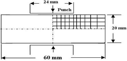
To illustrate the effectiveness of the ALE method in dynamic analysis, an example of punch indentation process solved by this approach is presented here. This example shows the robustness of this formulation in handling contact boundary conditions and in preventing mesh distortion. Both static and dynamic analyses are presented to show the significance of dynamic effects. Figure 3 shows the geometry and initial mesh of the
material. The material is assumed to be an elastic-plastic linear-hardening material with a Young’s modulus of 200 GPa, a Poisson’s ratio of 0.3, an initial yield stress of 250 MPa and a hardening parameter of 1.0 GPa.
Figure 3: Geometry and initial mesh for punch indentation
Figure 4 shows the evolution of the deformed shape obtained using the developed ALE formulation in static case. The figure shows that the contact condition between the punch and the workpiece is accurately satisfied. This was easily achieved by setting the degrees of freedom of the nodes directly under the punch to be Lagrangian in the vertical direction (to satisfy the boundary constraint) and Eulerian in the horizontal direction (to maintain the nodes under the punch). In this way, no special contact algorithm was needed to handle the contact conditions. In addition, using the designed mesh motion scheme, the ALE maintained a homogeneous mesh throughout the deformation history.
Figure 4: Evolution of the deformed shape during the punch indentation
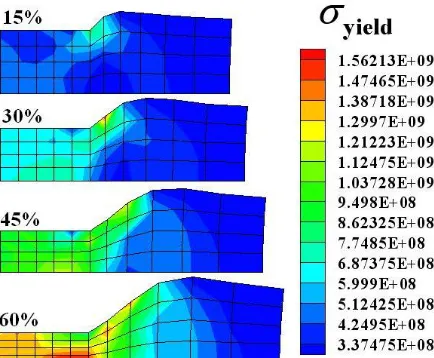
regularity and allows for an accurate description of the boundary motion. The evolution of the plastic areas starts from the right corner of the tool.
To investigate the dynamic effects, several punch velocities are simulated. Figure 6 shows the comparison between the final deformed shapes for various velocities. The dynamic effects are negligible for velocities under 2 m/s, but as the punch moves down at a faster rate, the plastic deformation is further localized because there is a shorter time for the plastic wave to propagate in the bulk of material. In other words, the final shape of the workpiece is clearly dependent on the punch velocity.
Figure 5: Evolution of the yield stress field during the deformation process
Figure 6: Deformed shape and equivalent plastic strain at different punch velocities
This type of problems is difficult to handle with a pure Lagrangian computation because several remeshing steps
are needed to overcome severe element distortions which are common to Lagrangian analysis. In addition, a contact algorithm may be needed to represent the motion of the die. Using the ALE method and its mesh motion scheme, the punch motion is simulated by directly applying appropriate velocity boundary conditions, and mesh distortion is avoided, resulting in a considerable computational saving.
The punch indentation problem has been repeatedly solved in the ALE literature, thus it is appropriate to compare the results with other references. It is apparent from Fig. 6. that the final length of the specimen (L) and its maximum height (H) are the two dimensions that are significantly affected by the punch speed. Therefore, they may be used as indicators for the forming of the specimen under dynamic loading.
TABLE 1
COMPARISON OF RESULTS FOR PUNCH INDENTATION
Reference _H(mm) Final _L(mm) Final Huerta A. and Gasadei F. [12]
Bayoumi H.N. and Gadala M.S. [13] Current work
11.0 11.0 11.5
36.5 43.0 37.75
Table (1) compares the values of these parameters for the case of punch speed of 60 m/s and after a punch advancement equivalent to 60% of initial height. It is observed that while the maximum height are almost the same for all cases, the specimen length is between the two other values reported, being closer to the value given in reference [13]. Furthermore, the distribution of yield stress and plastic strains presented in figures 5 and 6 are similar to those reported in the references.
8. CONCLUSIONS
9. REFERENCES
[1] M.S. Gadala, "Recent trends in ALE formulation and its applications in solid mechanics," Appl. Mech. Engrg. vol. 193, pp. 4247-4275, 2004.
[2] Benson DJ., "An efficient, accurate, simple ALE method for nonlinear finite element programs," Comput. Meth. Appl.Mech. Eng. Vol. 72, pp. 305–350, 1989.
[3] Haber RB., "A mixed Eulerian-Lagrangian displacement model for large-deformation analysis in solid mechanics," Comput. Meth. Appl. Mech. Eng. Vol. 43, pp. 277–292, 1984.
[4] Hue´tink J, Vreede PT, van der Lugt J, "Progress in mixed Eulerian-Lagrangian finite element simulation of forming processes", Int. J. Numer. Meth. Eng. Vol. 30, pp. 1441–1457,
1990.
[5] Kennedy JM, Belytschko TB, "Theory and application of a finite element method for arbitrary Lagrangian-Eulerian fluids and structures, " Nuc. Eng. Des. Vol. 68, pp. 129–146, 1981. [6] Schreurs PJG, Veldpaus FE, Brekelmans WAM, "Simulation of
forming processes using the arbitrary Eulerian- Lagrangian formulation," Comput. Meth. Appl. Mech. Eng. Vol. 58, pp. 19– 36, 1986.
[7] T.J.R. Hughes, W.K. Liu, T.K. Zimmermann, "Lagrangian-Eulerian finite element formulation for incompressible viscous flows," Comput. Methods Appl. Mech. Engrg. Vol. 29, pp. 329-349, 1981.
[8] J. Wang, M.S. Gadala, "formulation and survey of ALE method in nonlinear solid mechanics," Finite Element Anal. Des. Vol. 24, pp. 253-269 , 1997.
[9] Gadala, M.S. and Wang, J., "Apractical procedure for mesh motion in ALE method," Eng. With Computers, Vol. 14, pp. 223-234 , 1998.
[10] M.S. Gadala, M.R. Movahhedy, J. Wang, "On the mesh motion for ALE modeling of metal forming processes," Finite Elements in Analysis and Design, Vol. 38, pp. 435-459, 2002.
[11] R. Haber, M.S. Shepard, J.F. Abel, R.H. Gallagher, D.P. Greenberg, "A general two-dimentional, graphical finite element preprocessor utilizing discrete transfinite mapping," Int. J. Numer. Methods Engrg. Vol. 17, pp. 1015-1044, 1981.
[12] A. Huerta, F. Casadei, "New ALE applications in non-linear fast-transient solid dynamics, " Engineering Computations, Vol. 11, pp. 317-345, 1994.