journal homepage: http://jac.ut.ac.ir
Inverse eigenvalue problem for matrices whose graph is
a banana tree
M. Babaei Zarch
∗1, S. A. Shahzadeh Fazeli
†2and S. M. Karbassi
‡31,2,3
Department of Computer Science, Yazd University, Yazd, Iran. 2Parallel Processing Laboratory, Yazd University, Yazd, Iran.
ABSTRACT ARTICLE INFO
In this paper, we consider an inverse eigenvalue problem (IEP) for constructing a special kind of acyclic ces. The problem involves the reconstruction of matri-ces whose graph is a banana tree. This is performed by using the minimal and maximal eigenvalues of all lead-ing principal submatrices of the required matrix. The necessary and sufficient conditions for the solvability of the problem is derived. An algorithm to construct the solution is provided.
Article history:
Received 11, April 2018
Received in revised form 8, Au-gust 2018
Accepted 26 October 2018 Available online 30, December 2018
Keyword: Inverse eigenvalue problem; banana tree; leading principal minors; eigenvalue; graph of a matrix.
AMS subject Classification: 05C78.
1
Introduction
An inverse eigenvalue problem (IEP) concerns the reconstruction of a matrix from pre-scribed spectral data. In [3] detailed characterization of inverse eigenvalue problems is mentioned. Special types of inverse eigenvalue problems have attracted attention of many authors. Inverse eigenvalue problems for graphs have been studied in [4,7,8,10,12,13].
†Corresponding author: S. A. Shahzadeh Fazeli. Email: [email protected]
The inverse eigenvalue problem of a graph is to determine the possible spectra among real symmetric matrices whose pattern of nonzero off- diagonal entries is described by a graph. In the last fifteen years a number of papers on this problem have appeared. In this paper, we investigate an IEP, namely IEPB(c,s) (inverse eigenvalue problem for matrices whose graph is a banana tree). Similar problems were studied in [9,10,14]. For solving the problem, the recurrence relations among leading principal minors is used. Some ap-plications of the acyclic matrix discussed in this paper are in chemistry, energy and graph theory [1,5].
The paper is organized as follows. In Section 2, we give a brief outline of some preliminary concepts and clarify the notations used in the paper. In Section 3, we discuss the analysis of IEPB(c,s) and present an algorithm. In Section 4, we report numerical examples to illustrate the solutions of IEPB(c,s). In Section 5 conclusion is presented.
2
Preliminaries
Let Gbe a simple undirected graph (without loops and multiple edges) on n vertices. A real symmetric matrixA= (aij) is said to have a graph Gprovided aij 6= 0 if and only if
vertices iand j are adjacent in G.
Given an n ×n symmetric matrix A, the graph of A, denoted by G(A), has vertex set
V(G) = {1,2,3, . . . , n} and edge set E = {ij : i 6= j, aij 6= 0}. For graph G with n
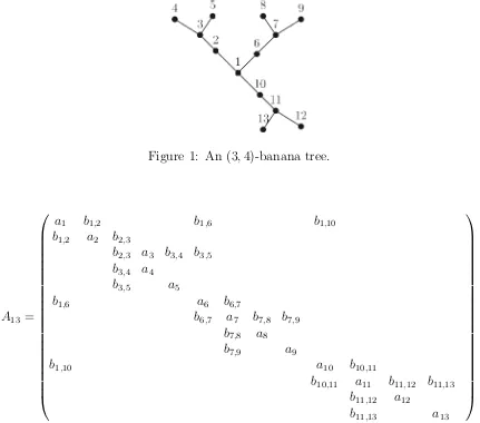
vertices, we denote by S(G) the set of all real symmetric matrices whose graph is G. A matrix whose graph is a tree is called an acyclic matrix. Some simple examples of acyclic matrices are the matrices whose graphs are paths,m-centipedes, brooms or banana tree. Definition 2.1. An (c, s)-banana tree, as defined by Chen et al.(1997), is a graph ob-tained by connecting one leaf of each of c copies of an s−star graph with a single root vertex that is distinct from all the stars.
Properties of banana trees have been studied in [2]. The vertices of an (c, s)-banana tree with c≥1, s≥3, labeled as follws:
The root vertex is labeled by 1, the vertices of distance 1 from the root vertex as the intermediate vertices is labeled by (i− 1)s + 2, the center of every (Ss) is labeled by
(i−1)s+ 3 and leaves of the center is labeled byj = (i−1)s+ 4, . . . , is+ 1, i= 1,2, . . . , c.
(Figure1).
Figure 1: An (3,4)-banana tree.
A13=
a1 b1,2 b1,6 b1,10
b1,2 a2 b2,3
b2,3 a3 b3,4 b3,5
b3,4 a4
b3,5 a5
b1,6 a6 b6,7
b6,7 a7 b7,8 b7,9
b7,8 a8
b7,9 a9
b1,10 a10 b10,11
b10,11 a11 b11,12 b11,13
b11,12 a12
b11,13 a13
where all theb’s are positive.
The following known results will be necessary for solving the problem in this paper. Lemma 2.2. [11] Let P(λ) be a monic polynomial of degree n with all real zeroes. Ifλ1 and λn are, respectively, the minimal and the maximal zero of P(λ), then
i. If x < λ1 , we have that (−1)nP(x)>0. ii. If x > λn , we have that P(x)>0.
Lemma 2.3. [6] (Cauchy’s interlacing theorem) Let λ1 ≤λ2 ≤. . .≤λn be the
eigenval-ues of an n×n real symmetric matrix A and µ1 ≤µ2 ≤. . .≤µn−1 be the eigenvalues of an (n−1)×(n−1) principal submatrix B of A, then
3
Problem statement and the solution
3.1
Problem statement
Given 2n−1 real numbers λ(1j),j = 1,2, . . . , n and λ(jj),j = 2, . . . , n, find an×n matrix
An ∈ S(B(c, s)) such that λ
(j)
1 and λ (j)
j are the minimal and maximal eigenvalues of Aj,
the leading principal submatrix ofA, respectively. This is referred toIEPB(c,s)problem. In the next subsection we discuss the solution of IEPB(c,s).
3.2
The solution of IEPB(c,s)
In the following, we investigate the relation between successive leading principal minors of λIn−An. Lemma 3.1 The sequence {Pj(λ) = det(λIj −Aj)}nj=1 of characteristic polynomials of Aj satisfies the following recurrence relations:
i. P1(λ) = (λ−a1)
ii. Pj(λ) = (λ−aj)Pj−1(λ)−b21,jdet(Bλj) j = (i−1)s+ 2, i= 1,2, . . . , c
iii. Pj(λ) = (λ−aj)Pj−1(λ)−b2(j−1),jPj−2(λ) j = (i−1)s+ 3, i= 1,2, . . . , c
iv. Pj(λ) = (λ−aj)Pj−1(λ)−b2(i−1)s+3,j P(i−1)s+2(λ)
Qj−1
k=(i−1)s+4(λ−ak)
j = (i−1)s+ 4, . . . , is+ 1, i= 1,2, . . . , c,
with the convention thatBjλis the submarix rows and columns 2,3, . . . , n−1 of the matrix
λIn−An, p0(λ) = 1 and Qj
−1
k=(i−1)s+4(λ−ak) = 1 when j = (i−1)s+ 4.
Proof. It is easy to verify by expanding the determinant.
Since λ(1j) and λ(jj) are eigenvalues of Aj, we have
(
Pj(λ(1j)) = 0
Pj(λ
(j)
j ) = 0.
(1)
Thus, solving the IEPB(c,s) is equivalent to solving the above system of equations for
j = 1,2, . . . , n. Observe that from the Cauchy’s interlacing property, the minimal and the maximal eigenvalue, λ(1j) and λ(jj), respectively, of each leading principal submatrix
Aj, j = 1,2, . . . , n, of the matrix A∈S(B(c, s)) satisfy the relations:
λ(1n) ≤λ(1n−1) ≤. . .≤λ1(2) ≤λ(1)1 ≤λ(2)2 ≤. . .≤λ(nn) (2) and
λ(1j) ≤ai ≤λ
(j)
j i= 1,2, . . . , j, j= 1,2, , . . . , n. (3)
Lemma 3.2. Let λ(1j) and λj(j) be the minimal and maximal eigenvalues of Aj for j =
Proof. Let Pj−1(λ (j)
1 ) and Pj−1(λ (j)
j ) be nonzero for j = (i −1)s + 2, i = 1,2, . . . , c,
replacing relation (ii) from Lemma 3.2 in equations (1), we obtain
Pj(λ
(j)
1 ) =ajPj−1(λ (j)
1 ) +b21,jdet(B λ(1j) j )−λ
(j)
1 Pj−1(λ (j) 1 ) = 0
Pj(λ
(j)
j ) =ajPj−1(λ (j)
j ) +b21,jdet(B λ(jj) j )−λ
(j)
j Pj−1(λ (j)
j ) = 0.
(4)
Which can be regarded as a linear system of equations inaj and b21,j. LetD1,j denote the
determinant of the system of equations (4), then
D1,j =Pj−1(λ (j)
1 )det(B
λ(jj)
j )−Pj−1(λ (j)
j )det(B λ(1j)
j ). (5)
Since b1,j’s are nonzero, from the relation (ii) of Lemma 3.2 we obtain the following:
det(Bjλ) = 1
b2 1,j
((λ−aj)Pj−1(λ)−Pj(λ)).
By replacing det(Bλ
(j) 1
j ) and det(B λ(jj)
j ) in D1,j and simplifying, we obtain
D1,j =
1
b2 1,j
Pj−1(λ (j)
j )Pj−1(λ (j) 1 )(λ
(j)
j −λ
(j)
1 )−Pj−1(λ (j) 1 )Pj(λ
(j)
j ) +Pj−1(λ (j)
j )Pj(λ
(j) 1 )].
Since Pj(λ
(j)
1 ) and Pj(λ
(j)
j ) are equal to zero and λ
(j)
1 and λ (j)
j are not roots of Pj−1(λ) then
D1,j =
1
b2 1,j
[Pj−1(λ(jj))Pj−1(λ(1j))(λ (j)
j −λ
(j) 1 )]6= 0.
Conversely, let D1,j 6= 0, if λ
(j) 1 =λ
(j−1)
1 then we have
det(Bλ
(j) 1
j ) = 0,
and this implies that D1,j = 0. But this contradicts our hypothesis that D1,j 6= 0. Hence
λ1(j) < λ(1j−1). Similarly, λj(j−−11) < λ(jj).
Lemma 3.3. Let A be a matrix of an (c, s)-banana tree and λ(1j), λ(jj) be the minimal and the maximal eigenvalue of the leading principal submatrix Aj of A, j = 2, . . . , n. If
λ1((i−1)s+2) < λ1((i−1)s+1) and λ(((i−i−1)1)ss+1+1) < λ(((i−i−1)1)ss+2+2), then we have
λ1(j) < λ(1j−1) , λj(j−−11) < λ(jj) (6)
and
λ1(j)< ak < λj(j) k = 1,2, . . . , j, (7)
Proof. Fori= 1,2, . . . , c, if j = (i−1)s+ 3, by Lemma 3.2 we have
P(i−1)s+3(λ) = (λ−a(i−1)s+3)P(i−1)s+2(λ)−b2(i−1)s+2,(i−1)s+3P(i−1)s+1(λ). (8)
If λ((1i−1)s+3) =λ((1i−1)s+2), by equation (8) we have
P(i−1)s+3(λ
((i−1)s+3)
1 ) =−b
2
(i−1)s+2,(i−1)s+3P(i−1)s+1(λ
((i−1)s+2)
1 ).
Sinceλ((1i−1)s+2) < λ1((i−1)s+1)thusP(i−1)s+1(λ
((i−1)s+2)
1 )6= 0 henceP(i−1)s+3(λ
((i−1)s+3) 1 )6= 0, but this is a contradiction, then we obtain λ((1i−1)s+3) < λ1((i−1)s+2). Similary, we have
λ(((ii−−1)1)ss+2+2) < λ(((ii−−1)1)ss+3+3).
Now we assume λ((1i−1)s+3) =a(i−1)s+3. Again, by equation (8) we have
P(i−1)s+3(λ
((i−1)s+3)
1 ) =−b
2
(i−1)s+2,(i−1)s+3P(i−1)s+1(λ
((i−1)s+3)
1 ).
Since λ1((i−1)s+3) < λ((1i−1)s+2) < λ1((i−1)s+1), we have P(i−1)s+1(λ
((i−1)s+3)
1 ) 6= 0 hence
P(i−1)s+3(λ
((i−1)s+3)
1 )6= 0 but this is a contradiction, then we obtainλ
((i−1)s+3)
1 < a(i−1)s+3. Similary, we havea(i−1)s+3 < λ
((i−1)s+3)
(i−1)s+3 , hence λ
((i−1)s+3)
1 < a(i−1)s+3 < λ
((i−1)s+3) (i−1)s+3 . If j = (i−1)s+ 4, by Lemma 3.2 we have
P(i−1)s+4(λ) = (λ−a(i−1)s+4)P(i−1)s+3(λ)−b2(i−1)s+3,(i−1)s+4 P(i−1)s+2(λ). (9)
If λ((1i−1)s+4) =λ((1i−1)s+3), by equation (9) we have
P(i−1)s+4(λ
((i−1)s+4)
1 ) = −b
2
(i−1)s+3,(i−1)s+4 P(i−1)s+2(λ
((i−1)s+3)
1 ).
Since λ((1i−1)s+3) < λ1((i−1)s+2) it means that λ1((i−1)s+3) is not a root of P(i−1)s+2(λ), then we obtain P(i−1)s+4(λ
((i−1)s+4)
1 ) 6= 0, this is a contradiction and λ
((i−1)s+4) 1 < λ
((i−1)s+3)
1 .
Similary, we haveλ(((i−i−1)1)ss+3+3) < λ(((i−i−1)1)ss+4+4). If λ((1i−1)s+4) =a(i−1)s+4 orλ
((i−1)s+4)
(i−1)s+4 =a(i−1)s+4 then by equation (9) we have
P(i−1)s+4(a(i−1)s+4) = −b2(i−1)s+3,(i−1)s+4 P(i−1)s+2(a(i−1)s+4).
Since λ1((i−1)s+4) < λ((1i−1)s+3)< λ1((i−1)s+2) then P(i−1)s+4(a(i−1)s+4)6= 0, which is a contra-diction. From (3) we have λ1((i−1)s+4)< a(i−1)s+4 < λ
((i−1)s+4) (i−1)s+4 .
Assume that (6), (7) hold for j = (i−1)s+ 5, . . . , isnow if j =is+ 1 by Lemma 3.2 we have
Pis+1(λ) = (λ−ais+1)Pis(λ)−b2(i−1)s+3, is+1 P(i−1)s+2(λ)
is
Y
k=(i−1)s+4
If λ(1is+1) =λ(1is), by equation (10) we have
Pis+1(λ (is+1)
1 ) =−b 2
(i−1)s+3, is+1 P(i−1)s+2(λ (is) 1 )
is
Y
k=(i−1)s+4
(λ(1is)−ak).
BecauseP(i−1)s+2(λ (is)
1 )6= 0 andλ (is)
1 < ak < λ
(is)
is , k = (i−1)s+4, . . . , is, then
Qis
k=(i−1)s+4(λ (is) 1 −
ak)6= 0 and we obtain Pis+1(λis1+1)6= 0. This is a contradiction andλ (is+1) 1 < λ
(is)
1 . Simi-lary, we have λ(isis)< λ(isis+1+1).
If λ(1is+1) =ais+1 orλ (is+1)
is+1 =ais+1 then by equation (10) we have
Pis+1(ais+1) =−b2(i−1)s+3, is+1 P(i−1)s+2(ais+1)
is
Y
k=(i−1)s+4
(ais+1−ak).
From the above verified results, we know
λ1(is+1) < λ(1is) < . . . < λ1((i−1)s+2) < . . . < λ(((i−i−1)1)ss+2+2) < . . . < λis(is) < λ(isis+1+1),
then P(i−1)s+2(ais+1) 6= 0 and we get Pis+1(ais+1) 6= 0. This is a contradiction and from (3) we have λ(1is+1) < ais+1 < λ
(is+1)
is+1 .
Theorem 3.4. The IEPB(c,s) has a unique solution if and only if
λ(1n)< λ(1n−1) < . . . < λ1(2) < λ(1)1 < λ(2)2 < . . . < λ(nn). (11)
Proof. First we assume that λ(1j) and λj(j) for all j = 1,2, . . . , n satisfying (11), thus
P1(λ (1)
1 ) = 0⇒a1 =λ (1) 1 .
For i = 1,2, . . . , c, if j = (i−1)s+ 2, by Lemma 3.2 we have D1,j 6= 0, by solving the
system (4) we obtain
aj =
λ(1j)Pj−1(λ (j)
1 )det(B
λ(jj) j )−λ
(j)
j Pj−1(λ (j)
j )det(B λ(1j) j )
D1,j
,
b21j = (λ (j)
j −λ
(j)
1 )Pj−1(λ (j)
1 )Pj−1(λ (j)
j )
D1,j
.
From equation (5) we have
(−1)j−1D1,j = (−1)j−1Pj−1(λ (j)
1 )det(B
λ(jj)
j ) + (−1) j−2
Pj−1(λ (j)
j )det(B λ(1j) j ).
From Lemma 2 and (11) we get (−1)j−1P
j−1(λ (j)
1 )>0,det(B
λ(jj)
j )>0,Pj−1(λ (j)
j )>0 and
(−1)j−2det(Bλ(1j)
b21,j = (−1)
j−1(λ(j)
j −λ
(j)
1 )Pj−1(λ(1j))Pj−1(λ(jj))
(−1)j−1P
j−1(λ(1j))det(B
λ(jj)
j ) + (−1)j−2Pj−1(λ(jj))det(B λ(1j) j )
>0.
Forj = (i−1)s+ 3 the existence ofAj is equivalent to show that the system of equations
(
Pj(λ
(j)
1 ) = ajPj−1(λ (j)
1 ) +b2(j−1),jPj−2(λ (j) 1 )−λ
(j)
1 Pj−1(λ (j) 1 ) = 0
Pj(λ
(j)
j ) =ajPj−1(λ (j)
j ) +b2(j−1),jPj−2(λ
(j)
j )−λ
(j)
j Pj−1(λ (j)
j ) = 0,
(12)
has solutions aj and b2(j−1),j. The determinant of the coefficients matrix of the above
system is
D(j−1),j =Pj−1(λ (j)
1 )Pj−2(λ (j)
j )−Pj−1(λ (j)
j )Pj−2(λ (j) 1 ).
If D(j−1),j 6= 0 then the system will have a unique solution. From Lemma 2 and (11)
we get (−1)j−1D
(j−1),j > 0, it is clear that D(j−1),j 6= 0 and the unique solutions of the
system (12) are:
aj =
λ(1j)Pj−1(λ (j)
1 )Pj−2(λ (j)
j )−λ
(j)
j Pj−1(λ (j)
j )Pj−2(λ (j) 1 )
D(j−1),j
,
b2(j−1),j =
(λ(jj)−λ1(j))Pj−1(λ(1j))Pj−1(λ(jj))
D(j−1),j
.
Again, from Lemma 2 and (11) we have (−1)j−1P
j−1(λ (j)
1 ) >0 and Pj−1(λ (j)
j )> 0, then
it is evident that:
b2(j−1),j = (−1)
j−1(λ(j)
j −λ
(j)
1 )Pj−1(λ (j)
1 )Pj−1(λ (j)
j )
(−1)j−1P
j−1(λ (j)
1 )Pj−2(λ (j)
j ) + (−1)j−2Pj−1(λ (j)
j )Pj−2(λ (j) 1 )
>0.
Finally, forj = (i−1)s+ 4, . . . , is+ 1, using the last recurrence relation from Lemma 3.2 in equations 1 we have
(
ajPj−1(λ (j)
1 ) +b2((i−1)s+3),jP(i−1)s+2(λ
(j) 1 )
Qj−1
k=(i−1)s+4(λ (j)
1 −ak)−λ
(j)
1 Pj−1(λ (j) 1 ) = 0
ajPj−1(λ (j)
j ) +b2((i−1)s+3),jP(i−1)s+2(λ (j)
j )
Qj−1
k=(i−1)s+4(λ (j)
j −ak)−λ
(j)
j Pj−1(λ (j)
j ) = 0.
(13) The determinant of the coefficients matrix of the system (13) is
D(i−1)s+3, j =
Pj−1(λ (j)
1 )P(i−1)s+2(λ (j)
j )
Qj−1
k=(i−1)s+4(λ (j)
j −ak)
−
Pj−1(λ (j)
j )P(i−1)s+2(λ (j) 1 )
Qj−1
k=(i−1)s+4(λ (j) 1 −ak)
.
(14)
From (14 ) we have
(−1)j−1D
(i−1)s+3, j =
(−1)j−1P
j−1(λ (j)
1 ) P(i−1)s+2(λ (j)
j )
Qj−1
k=(i−1)s+4(λ (j)
j −ak)
+
Pj−1(λ (j)
j )
(−1)(i−1)s+2P
(i−1)s+2(λ (j)
1 ) (−1)j
−(i−1)s−4Qj−1
k=(i−1)s+4(λ (j) 1 −ak)
.
By Lemma 2 and (11) we get (−1)j−1P
j−1(λ (j)
1 )>0,Pj−1(λ (j)
j )>0, (−1)(i
−1)s+2P
(i−1)s+2(λ (j) 1 )> 0 and P(i−1)s+2(λ
(j)
j )> 0. Also, by Lemma 3.2, we have (−1)j−(i−1)s−4
Qj−1
k=(i−1)s+4(λ (j) 1 −
ak)>0 and
Qj−1
k=(i−1)s+4(λ (j)
j −ak)>0.Hence, (−1)j−1D(i−1)s+3), j >0 andD(i−1)s+3, j 6= 0.
It follows that the linear sysyem equations (13) has a unique solution foraj andb2(i−1)s+3, j.
aj =
Aj −Bj
D(i−1)s+3, j
,
b2(i−1)s+3, j = (λ (j)
j −λ
(j)
1 )Pj−1(λ (j)
1 )Pj−1(λ (j)
j )
D(i−1)s+3, j
,
where Aj and Bj are given by
Aj =λ
(j)
1 Pj−1(λ (j)
1 )P(i−1)s+2(λ (j)
j ) j−1 Y
k=(i−1)s+4
(λ(jj)−ak),
Bj =λ
(j)
j Pj−1(λ (j)
j )P(i−1)s+2(λ (j) 1 )
j−1 Y
k=(i−1)s+4
(λ(1j)−ak).
We can write b2
(i−1)s+3, j as:
b2(i−1)s+3, j = (λ (j)
j −λ
(j) 1 )
(−1)j−1P
j−1(λ (j)
1 )Pj−1(λ (j)
j )
(−1)j−1D
(i−1)s+3, j
.
From Lemma 2 and (11) we have (−1)j−1Pj−1(λ (j)
1 ) >0 and Pj−1(λ (j)
j ) > 0. Also, from
the above verified results, we know (−1)j−1D
(i−1)s+3, j >0, hence b2(i−1)s+3, j >0.
Conversely, suppose the IEPB(c,s) has a unique solution then from Lemma 3.2 and Lemma 3.2 we can obtain (11) thus the proof is completed.
Algorithm 1. (To solve problem IEPB(c,s))
Input: c, s, λ(1)1 , λ(2)1 , λ(2)2 , . . . , λ1(n), λ(nn), where n=cs+ 1.
Output: A∈S(B(c, s)).
a1 =λ (1) 1 .
Forj = 2 to n
if j ∈(i−1)s+ 2 f or i= 1,2, . . . , c Then
aj =
λ(1j)Pj−1(λ(1j))det(B
λ(j) j j )−λ
(j)
j Pj−1(λ(jj))det(B
λ(j)
1
j )
D1,j
b1,j =
r
(λ(jj)−λ1(j))Pj−1(λ (j)
1 )Pj−1(λ(jj))
D1,j
elseif j ∈(i−1)s+ 3 f or i= 1,2, . . . , c then
aj =
λ1(j)Pj−1(λ1(j))Pj−2(λ(jj))−λj(j)Pj−1(λj(j))Pj−2(λ(1j))
D(j−1),j
b(j−1),j =
r
(λ(jj)−λ(1j))Pj−1(λ(1j))Pj−1(λ(jj))
D(j−1),j
else
f or j = (i−1)s+ 4 to is+ 1, i= 1,2, . . . , c do aj =
Aj−Bj
D(i−1)s+3, j
b(i−1)s+3, j =
r
(λ(jj)−λ(1j))Pj−1(λ(1j))Pj−1(λ(jj))
D(i−1)s+3, j
EndIf EndFor
4
Numerical examples
Algorithm 1is tested for various examples by matlab software. In this section we report some of examples. Example 4.1For given 17 real numbers
−7,−6.1,−5,−3.6,−2.5,−1,−0.5,1.5, 2, 2.5, 3, 4, 5.3, 6, 7, 8, 9.2,
rearrange and label them as λ(1j), j = 1,2, . . . ,9 and λ(jj), j = 2, . . . ,9, and find a matrix 9×9∈S(B(2,4)) such thatλ1(j) andλ(jj) are the minimal and maximal eigenvalues of Aj,
j = 1,2, . . .9.
We rearrange the given numbers. The following numbers:
satisfy the sufficient condition (11). By applyingAlgorithm 1, we get the unique solution
A9 =
2.0000 0.5000 0 0 0 4.6952 0 0 0 0.5000 2.0000 1.4142 0 0 0 0 0 0 0 1.4142 0.3333 1.6101 3.0587 0 0 0 0 0 0 1.6101 3.0029 0 0 0 0 0 0 0 3.0587 0 2.3925 0 0 0 0 4.6952 0 0 0 0 0.3752 3.6226 0 0
0 0 0 0 0 3.6226 0.9421 5.0534 4.4313 0 0 0 0 0 0 5.0534 1.1223 0 0 0 0 0 0 0 4.4313 0 2.2202
.
From the matrixA9 we recomputed the eigenvalues ofAj, and obtained
σ(A1) ={2.0000}
σ(A2) ={1.5000,2.5000}
σ(A3) ={−0.5000,1.8333,3.0000}
σ(A4) ={−1.0000,1.7143,2.6219,4.0000}
σ(A5) ={−2.5000,1.5649,2.4890,2.8749,5.3000}
σ(A6) ={−3.6000,−2.4916,2.0448,2.8688,5.2820,6.0000}
σ(A7) ={−5.0000,−2.4970,1.2356,2.1448,2.8698,5.2929,7.0000}
σ(A8) ={−6.1000,−2.5108,−2.1528,2.0401,2.8686,4.7171,5.3061,8.0000}
σ(A9) ={−7.0000,−2.6646,−2.4642,1.7361,2.0463,2.8688,5.2344,5.4318,9.2000}.
The underlined eigenvalues are in consonance with the minimal and maximal eigenvalues. Example 4.2. For given 11 real numbers
−8,−6,−3,−1, 1, 2, 5, 6, 8, 11, 13,
rearrange and label them as λ(1j), j = 1,2, . . . ,6 and λ(jj), j = 2, . . . ,6, and find a matrix 6×6∈S(B(1,5)) such thatλ1(j) andλ(jj) are the minimal and maximal eigenvalues of Aj,
j = 1,2, . . .6.
We rearrange the given numbers. The following numbers:
−8<−6−1<1<2<5<6<8<11<13,
satisfy the sufficient condition (11). By applyingAlgorithm 1, we get the unique solution
A6 =
2.0000 1.7321 0 0 0 0 1.7321 4.0000 2.5820 0 0 0
0 2.5820 0.6667 4.4117 6.5160 6.1730 0 0 4.4117 4.4146 0 0 0 0 6.5160 0 4.3427 0 0 0 6.1730 0 0 4.3356
.
From the matrixA6 we recomputed the eigenvalues ofAj, and obtained
σ(A2) ={1.0000,5.0000}
σ(A3) ={−1.0000,1.6667,6.0000}
σ(A4) ={−3.0000,1.2100,4.8713,8.0000}
σ(A5) ={−6.0000,1.0811,4.3918,4.9511,11.0000}
σ(A6) ={−8.0000,1.0521,4.3389,4.3999,4.9686,13.0000}.
The underlined eigenvalues are in consonance with the minimal and maximal eigenvalues.
5
Conclusions
In this paper, we have solved the IEP for construction of matrices whose graphs are banana trees. This is performed by using the minimal and maximal eigenvalues of all leading principal submatrices of the required matrix. The results obtained in this paper provide an efficient method for constructing such matrices. The problem IEPB(c,s) is important in the sense that it partially describes inverse eigenvalue problem while it constructs matrices from partial information of prescribed eigenvalues. Such partially described problems may occur in computations involving a complex physical system that is difficult to obtain in its entire spectrum. It would be interesting to consider such IEPs for other acyclic matrices as well.
References
[1] Asmiati, Locating chromatic number of banana tree, International Mathematical Forum 12 (2017) 39-45.
[2] Chen, W.C., Lu, H. I., and Yeh, Y. N., Operations of interlaced trees and graceful trees,Math 21(1997).
[3] Chu, M. T., and Golub, G. H., Inverse Eigenvalue Problems: Theory, Algorithms and Application, Oxford University Press, New York, (2005).
[4] Duarte, A.L., Construction of acyclic matrices from spectral data, Linear Algebra and its Applica-tions 113(1989) 173-182.
[5] Gutman, I., and Triantallou, I., Dependence of graph energy on nullity: A case study, Communica-tions in Mathematical and in Computer Chemistry 76(2016).
[6] Hogben, L., Spectral graph theory and the inverse eigenvalue problem of a graph, Electronic Journal of Linear Algebra 14(2005), 12-31.
[7] Monfared, K. H., and Shader B.L., Construction of matrices with a given graph and prescribed interlaced spectral data, Linear Algebra and its Applications 438(2013) 4348-4358.
[8] Nair, R., and Shader B.L., Acyclic matrices with a small number of distinct eigenvalues, Linear Algebra and its Applications 438(2013) 4075-4089.
[10] Peng, J., Hu, X., and Zhang, L., Two inverse eigenvalue problems for a special kind of matrices, Linear Algebra and its Applications 416 (2006) 336-347.
[11] Pickmann, H., Egana, J., and Soto, R.L., Extremal inverse eigenvalue problem for bordered diagonal matrices, Linear Algebra Applications 427 (2007).
[12] Sen, M., and Sharma, D., Generalized inverse eigenvalue problem for matrices whose graph is a path, Linear Algebra and its Applications 446 (2014) 224-236.
[13] Sharma, D., and Sen, M., Inverse eigenvalue problems for acyclic matrices whose graph is a dense centipede De Gruyter 6 (2018 )77-92