Pareto design of fuzzy tracking control based on particle swarm optimization algorithm for a walking robot in the lateral plane on slope

AUT J. Model. Simul., 50(2) (2018) 157-164 DOI: 10.22060/miscj.2018.14327.5103

Pareto design of fuzzy tracking control based on particle swarm optimization algorithm

for a walking robot in the lateral plane on slope

M.J. Mahmoodabadi1*_{, M. Taher-Khorsandi}2

1 _{Department of Mechanical Engineering, Sirjan University of Technology, Sirjan, Iran}

2 _{Department of Mechanical Engineering, University of Texas at San Antonio, San Antonio, USA}

ABSTRACT: Many researchers have controlled and analyzed biped robots that walk in the sagittal plane. These robots require the capability of walking merely laterally when they are faced with the obstacles such as a wall. In this field of study, both nonlinearity of the dynamic equations and also having a tracking system cause an effective control has to be utilized to address these problems. Therefore, this paper presents a nonlinear fuzzy tracking control for the walking robots that step in the lateral plane on a slopes. When fuzzy control is utilized to track the desired trajectories of the joints, there has to be a trade-off between tracking errors and control efforts. Consequently, a particle swarm optimization algorithm is used to obtain the Pareto front of these non-commensurable objective functions to determine the fuzzy control parameters. In this paper, normalized summation of angle errors and normalized summation of control efforts are considered as the objective functions. These objective functions have to be minimized simultaneously. A vector which contains the control parameters is considered as the vector of selective parameters with positive constant values. The obtained Pareto front by the proposed multi-objective algorithm is compared with three prominent algorithms, modified NSGAII, Sigma method and MATLAB Toolbox MOGA. The result dramatizes the superiority of innovative particle swarm optimization over the algorithms.

Review History: Received: 15 April 2018 Revised: 4 October 2018 Accepted: 14 October 2018 Available Online: 19 October 2018

Keywords: Walking Robot Fuzzy Tracking Control Particle Swarm Optimization Multi-objective Optimization

1- Introduction

The challenging walking robot field has attracted the interest of many researchers for several decades. The dynamic of this sort of robot is extremely nonlinear and difficult to control since researchers confront with a heavy nonlinearity in the dynamic equations which must track the desired trajectory. Lately, fuzzy control has been utilized by researchers as an effective control to satisfy criteria for nonlinearity of dynamic equation and tracking system. Liu et al. [1] illustrated that the fuzzy control could be utilized to control the walking robots. Li et al. [2] considered a robot walking in the sagittal plane in its desired ZMP and utilized a fuzzy motion control based on reinforcement learning and Lagrange polynomial interpolation for gait synthesis of walking robots. The most appropriate stability criterion is Zero Moment Point (ZMP). This criterion does take dynamic forces, as well as static forces, into consideration. Goswami et al. [3] computed ZMP by an approximation-based method and they optimized walking parameters such as step-length, bending-height, etc. Some studies introduced the concept of combined trajectory paths, Naseradin mousavi et al. [4] illustrated that hip height plays an important role in both the stability and optimum actuator torques of the joints. All the above-mentioned works have studied walking robots that walk in the sagittal plane, but they did not study walking in the lateral plane. Ito et al. [5] proposed a static balance control based on the feedback of ZMP positions and extended these methods to the walking in-place lateral stepping motion; however, they did not study the walking of the robot in that plane.

Taher Khorsandi et al. [6] introduced the motion of the

walking robot in the lateral plane and linearized the dynamical equations of the robot in the trajectory and utilized linear quadratic tracking control to control them. Their work would be developed by the present study. They linearized the dynamical equation to control the robots; however, in this study a nonlinear fuzzy tracking control is used to control them and linearization would be relaxed. They considered a flat surface while in this paper, the robot walks on slope. Furthermore, an innovative optimization method is utilized to optimize the control parameters.

The parameters of fuzzy tracking control have to be determined and they are usually identified by trial-and-error process. One proper way to choose these factors is using an evolutionary algorithm such as particle swarm optimization, genetic algorithm and etc. Shook et al. [7] used genetic algorithm to optimize fuzzy logic controllers which were designed to manage two 20 kN magnetorheological dampers for mitigation of seismic loads. Shayeghi et al. [8] proposed a multi-stage fuzzy controller for solution of the load frequency control which operated under deregulation and also the membership functions were designed automatically by particle swarm optimization (PSO). Bingul [9] controlled a 2-DOF planer robot by fuzzy logic controller, and particle swarm optimization was utilized to tune fuzzy parameters. A PID controller was also tuned by particle swarm optimization to contrast with the fuzzy controller. Therefore, an innovative particle swarm optimization presented in this paper is utilized to eliminate the boring and repetitive trial-and-error process and to find the fuzzy parameters.

It was developed through simulation of simplified social systems, and has been found to be robust in solving nonlinear optimization problems [11]. The PSO technique can generate a high quality solution with short calculation time and a more stable convergence characteristic compared to other evolutionary methods [12,13]. In this paper, for increasing the convergence of the population and to avoid local minima, PSO is merged with convergence and divergence operators. In the recent years, several approaches have been proposed to extend the PSO algorithm to deal with multi-objective optimization problems. For instance, dynamic neighborhood PSO [14], dominated tree [15], Sigma method [16], and vector evaluated PSO [17] have been proposed to solve the multi-objective optimization problems.

This research paper develops considerably the authors’ previous study [6] in the aspect of proposing the fuzzy tracking control optimized by multi-objective particle swarm optimization as an effectual controller for a walking robot that walks merely on the lateral plane of a slope. As a noteworthy development, optimal fuzzy tracking control based upon particle swarm optimization is proposed here to control effectively the walking of the biped robot in the lateral plane of a slope.

2- The model of the walking robot

A three link planar model in the lateral plane is used to model the robot [6]. The first link is anchored to the ground surface while the third link moves freely along lateral plane and the second link represents the head, arms and trunk. Each link is defined by four characteristics, that are mass, length, inertia and the center of gravity. The variable joints for this robot are regarded as θ₁,

θ

₂ and

θ

₃. The numerical values of the related parameters are exactly considered same as those in [18]. The dynamical equations of the robot’s motion can be derived by using the Newton-Euler or the Lagrange-Euler formalisms as those in [6].

3- Fuzzy tracking control of walking robot

The proposed fuzzy tracking control is based on the closed-loop fuzzy system. The stages of the control method was designed and constructed step by step as follows. To control the system, the state variable vector is chosen as

[

x x x x x x1, , , , ,2 3 4 5 6

]

= θ θ θ θ θ θ1, , , , ,1 2 2 3 3. The errors could be defined as follows.

(

)

(

)

1,2,3 1,2,3

p dp p

q dq q

E p

E q

θ θ

θ θ

= − =

=  −  = (1) The new error indexes parameters would be introduced as:

( )

p dp p 1,2,3 Ep

dp p dp p

E

Index θ θ p

θ θ θ θ

−

= = =

+ +

( )

q dq q 1,2,3 Eq

dq q dq q

E

Index θ θ q

θ θ θ θ

−

= = =

+ +

 

   

(2)

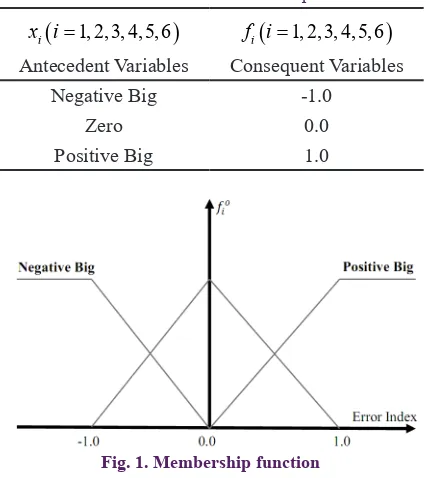
Then, a membership function is constructed by Fig. 1 illustrated by Table 1. In the Fig. 1, the inference result

o i

f of the consequent variable f_i should be calculated by the product-sum gravity method [19] via the following formulation.

(

)

(

)

(

)

3 1 3 1

i i E

o i

i E _i

E i

y Index

f Index

Index µ µ =

=

=

∑

∑

(3)

where _yi _{is the center of an output membership function and} i

µ is an input membership function.

Finally, the control efforts are obtained by the following equation.

1 1 1 2 2

u w f w f= +

2 3 3 4 4

u =w f w f+ (4)

3 5 5 6 6

u =w f +w f

In this equation, w w w w w1, , , , , 2 3 4 5 and w6 are weight constants

and these parameters are usually identified by trial-and-error process. One proper way to choose these factors is using evolutionary algorithms. Therefore, an innovative particle swarm optimization presented in this paper is utilized to eliminate the boring and repetitive trial-and-error process and to find fuzzy parameters w ii

(

=1,2,3,4,5,6

)

.

4- Single objective optimization algorithm 4- 1- Particle swarm optimization

Particle swam optimization is a population-based evolutionary algorithm and is similar to other population based evolutionary algorithms. PSO is motivated by the simulation of social behavior instead of survival of the fittest [10]. Although originally adopted for balancing weights in neural networks [20], PSO soon became a very popular global optimizer, mainly in problems in which the decision variables are real numbers [21].

In PSO, each candidate solution is associated with a velocity. The candidate solutions are called particles and the position of each particle is changed according to its own experience and that of its neighbors (velocity). It is expected that the particles will move towards better solution areas. Mathematically, the particles are manipulated according to the following equations,

1 1

i i i

x ( t→ + =) x ( t ) v ( t→ +→ + ), (5)

1 1 2 2

1 pbesti gbest

i i i i

v ( t→ + =) W v ( t ) C r ( x→ + → −x ( t )) C r ( x→ + → −x ( t )),→ (6) where xi(t)

→

and vi(t)

→

denote the position and velocity of Fig. 1. Membership function

Table 1. Rule modules for each input item.

(

)

1,2,3,4,5,6

i

x i=

Antecedent Variables

(

1,2,3,4,5,6

)

i

f i=

Consequent Variables

Negative Big -1.0

Zero 0.0

particle i, at time step t. r1,r2∈[01,]are random values. C1

is the cognitive learning factor and represents the attraction that a particle has toward its own success. C₂ is the social learning factor and represents the attraction that a particle has toward the success of the entire swarm. W is the inertia weight which is employed to control the impact of the previous history of velocities on the current velocity of a given particle. The personal best position of the particle i is

i

pbest

x

→

, and xgbest

→

is the position of the best particle of the entire swarm. Inertia weight is used to balance the global and local search ability.

The characteristics of the inertia weight are similar to those of the temperature parameter in the simulated annealing algorithm [12]. A large inertia weight facilitates a global search while a small inertia weight facilitates a local search. By changing the inertia weight dynamically, the search ability is dynamically adjusted. Experimental results indicated that the linearly decreasing inertia weight over the iterations improve the performance of PSO [21]. With a large value of

1

C and a small value of C₂, particles are allowed to move around their personal best position (xpbesti

→

). With a small value of C₁ and a large value of

2

C , particles converge to the best particle of the entire swarm (xgbest

→

). From the results, it was observed that best solutions were determined when C₁ is linearly decreased and C₂ is linearly increased over the iterations [22]. Hence, in this paper, the following linear formulation for inertia weight and learning factors are used.

(

)

1 1 2 t ,

W W W W

maximumiteration

 

= − − _{× }

  (7)

(

)

1 1i 1i 1f t ,

C C C C

maximumiteration

 

= − − _{× }

  (8)

(

)

2 2i 2i 2f t ,

C C C C

maximumiteration

 

= − − _{× }

  (9) where W1 and W2 are the initial and final values of the inertia

weight, respectively. C_1i and C_2i are the initial values of the learning factors C1 and C2, respectively. C1f and C2f are the

final values of the learning factors C₁ and C₂, respectively. t is the current iteration number and maximumiteration is the maximum number of allowable iterations.

4- 2- Convergence operator

A novel convergence formula that contains four parent particles has been proposed in [23,24]. Let 0,1ρ∈

[ ]

be a random number. If ρ ≤P_Convergence (P_Convergence is convergence probability), then, one of the following operators shall be performed to generate the new particle position x ti

(

+1

)

from the old particle position x ti

( )

:

If fitness x t_i

( )

is smaller than fitness x t_j

( )

and fitness

( )

k

x t then:

(

1

)

1 gbest

_{( )}

(

2

( )

( )

( )

)

i gbest i j k

i

x

x t x x t x t x t

x t

σ  

+ = + _ _ − −

 



    

 (10)

If fitness x t_j

( )

smaller than fitness x t_i

( )

and fitness x t_k

( )

then:

(

1

)

2 gbest

_{( )}

(

2

( )

( )

( )

)

i gbest j i k

i

x

x t x x t x t x t

x t

σ  

+ = + _ _ − −

 



    

 (11)

If fitness x t_k

( )

is smaller than fitness x t_j

( )

and fitness

( )

i

x t then:

(

1

)

3 gbest

_{( )}

(

2

( )

( )

( )

)

i gbest k j i

i

x

x t x x t x t x t

x t

σ  

+ = + _ _ − −

 



    

 (12)

where particles x t_j

( )

and x t_k

( )

are selected from swarm by uniformly selection method. σ1, σ2, and σ3 are random

numbers selected from

[ ]

0,1 and x_gbestis the position of the best particle of the entire swarm. After calculating the convergence phase, the superior member between x t_i

( )

and x ti

(

+1

)

should be selected. If ρ≥PConvergence, then no

convergence operation is performed for x t_i

( )

. 4- 3- Divergence Operator

This operator, that was proposed in [23,24], provides a possible leap on some chosen particles . Let 0,1ϑ∈

[ ]

be a random number. If ϑ≤P_Divergence, (P_Divergence is divergence probability) and particle x t_i

( )

was not enhanced by convergence operator, then the following divergence operator is performed to generate a new particle.

(

1

)

(

( )

,

)

.

i i D

x t + =Normrand x t S (13)

( )

(

)

,i D

Normrand x t S generates random numbers from the normal distribution with mean parameter x t_i

( )

and standard deviation parameter S_D (S_D is a positive constant). If

Divergence P

ϑ≥ or particle x t_i

( )

was enhanced by convergence operator, no divergence operation is performed.

4- 4- Hybrid of PSO, Convergence, and Divergence Operators It is now possible to present a novel PSO which is improved by utilizing the convergence and divergence operators to update the particle positions. Initially, particles forming the population are randomly generated. Then, convergence and divergence probabilities, the inertia weight and the learning factors are selected. In each iteration, after calculation of the fitness values of all particles, x_pbestiand x_gbestare determined. Then, for each particle a random number ρ∈

[ ]

0,1 would be allocated. If a particle has ρ ≤PC, a new particle will

be produced by the convergence operator. For each particle that is not chosen for convergence operation another random number ϑ 0,1∈

[ ]

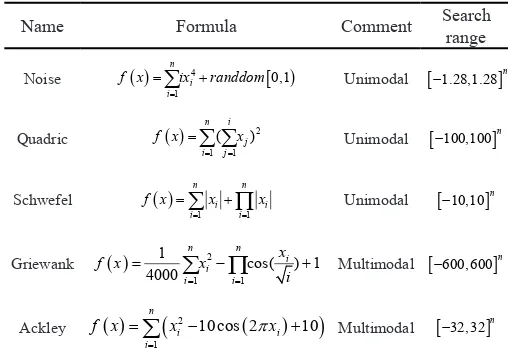
would be allocated. If ϑ ≤P_D then the divergence operator generates a new particle. Other particles that are not selected for convergence or divergence operation will be enhanced by PSO. This cycle should be repeated until the user-defined stopping criterion is satisfied [23,24].

Table 2. Optimization benchmark test functions Name Formula Comment Search _range

Noise ( ) 4 [ )

1 0,1

n i i

f x ix randdom

=

=∑ + Unimodal [₋1.28,1.28]n

Quadric ( ) 2

1 1

( )

n i j i j

f x x

= =

=

∑ ∑

_{Unimodal [} 100,100_]n

−

Schwefel ( )

1 1

n n

i i

i i

f x x x

= =

=∑ +∏ Unimodal [₋10,10]n

Griewank ( ) 2

1 1

1 _{cos( ) 1}

4000

n n

i i

i i

x

f x x

i

= =

=

∑ ∏

− + Multimodal [ 600,600]n

−

Ackley ( )

(

2 ( )

)

1

10cos 2 10 n

i i

i

f x x πx

=

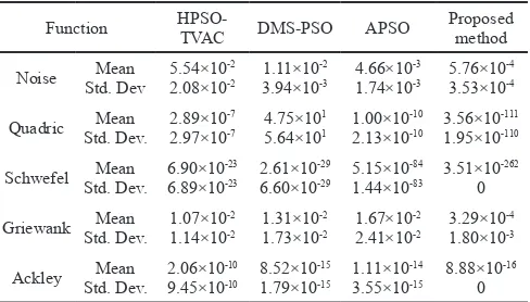
4- 5- Evaluation of single objective optimization algorithm To evaluate the accuracy of the proposed method, three renowned PSO algorithms are used for comparison, (HPSO-TVAC [22], DMS-PSO [25], and APSO [26]). Moreover, five nonlinear benchmark functions introduced in Table 2 are performed. These test functions should be minimized. In all the tests, the inertia weight W is linearly decreased from W₁=0.9 to W₂ =0.4, C₁ is linearly decreased from

1i 2.5

C = to C₁f =0.5 while C2 is linearly increased from

2i 0.5

C = to C₂f =2.5 over time. The related variables used in

convergence and divergence operators are: P_Convergence =0.02

and PDivergence=0.02. Furthermore, the term v ti

( )

is limited

to the range

[

−vave,+vave

]

which vave=xmax₂−xmin. While the velocity violates this range, it will be multiplied by a random number between

[ ]

0,1.

The mean and standard deviation fitness of the best particle for thirty runs are summarized in Table 3. The population size, maximum iteration and dimension are set at 20, 10000 and 30, respectively. It can be observed from this table that the incorporation of the convergence and the divergence operators can greatly change the performance of PSO. From the results given in Table 3, it can be seen that the proposed method outperforms other three algorithms for different complex functions. Obviously, the technique of combination of PSO, convergence and divergence operators improves PSO and make the swarm easily escape from the local minima and converge to the global minimum, robustly. 5- Multi-objective optimization algorithm

Moore and Chapman proposed the first extension of the PSO strategy for solving multi-objective problems in an unpublished manuscript in 1999 [27]. After this early attempt, a great interest to extend PSO arose among researchers, but interestingly, the next proposal was not published until 2002. Nevertheless, there are currently different proposals of multi-objective PSOs reported in the specialized literature [28]. 5- 1- Definitions of multi-objective optimization problem A multi-objective optimization problem is of the following form,

Minimize →f(→x):=[f₁(→x), f₂(→x),...,fk(→x)] (14)

where T

n x x x

x=[ ₁, ₂,..., ]

→

is the vector of decision variables,

k i R R

f n

i: → , =1,..., are the objective functions. To

describe the concept of optimality, some definitions should be introduced.

Definition 1. Given two vectors →_x,→_y∈Rk_{, we say that}

→ →

≤ y

x if xi yi

→ →

≤ for i=1,...,n and that →x _dominates →y (denoted by →x→y) if →x≤→y _and →x≠→y [29].

Definition 2. A vector of decision variables →_{x∈χ ⊂R}n

is non-dominated with respect toχ, if there does not exist another →_x′∈χ _{such that}→_f(→_x′_)→_f(→_x) [29].

Definition 3. A vector of decision variables _x→∗_∈F⊂Rn _(F

is the feasible region) is Pareto-optimal if it is non-dominated with respect to F [29].

Definition 4. The Pareto optimal set _p∗_{is defined by [29]:}

{ }

p∗₌ →x F | x is Pareto optimal_∈ →

(15)

Definition 5. The Pareto front pF∗

is defined by [29]:

{ ( ) k| }

pF∗₌ → →f x _∈R x p→_∈ ∗

(16) Thus, determination of the Pareto optimal set from the set F of all the decision variable vectors is desired [29].

5- 2- Multi-objective CDPSO

When solving single-objective optimization problems by PSO approach,xgbest

→

is used as a leader to update particles position. However, in the case of multi-objective optimization problems, each particle might have a set of different leaders (each non-dominated solution could be selected as a leader) which only one of them can be selected in order to update its position. In this paper, we describe a leader selection technique that is based on the density measures. For this purpose, a neighborhood radius R_neighborhood is defined for leaders. Two leaders are neighbors if their Euclidean distance (measured in the objective domain) is less than R_neighborhood. Using this definition, the number of neighbors of each leader is calculated in the objective function domain. The particle which has fewer neighbors is preferred as leader. However, after several iterations, the leader position and its density will change. Thus, leader selection operation should be repeated and a new leader must be identified. Therefore, the maximum iteration is divided into several equal periods, and each period has the same iterationT. The relationship of maximum iteration, number of periods and T satisfies the following equation.

maximum iteration number of periods = ×T (17) In each period, the leader selection operation could be done and the non-dominated solution which has fewer neighbors is preferred as leader. Also, in the start of each iteration of a period, if a particle dominates the leader, then this particle will be considered as the new leader. This algorithm is named periodic objective optimization. The proposed multi-objective method allows us to independently select inertia weight and learning factors in each period. The following equations are suggested to select the inertia weight and learning factors in each period.

(

)

1 2 1 _Tt t_T1

W W= + W W− _ − fix_ − __

 

  (18)

(

)

1 1i 1f 1i _Tt t_T1

C C= + C −C _ − fix_ − __

 

  (19)

(

)

2 2i 2f 2i _Tt t_T1

C =C + C −C _ −fix_ − __

 

  (20) Table 3. Comparison results on accuracy of algorithms

Function HPSO-_TVAC DMS-PSO APSO Proposed _method

Noise _{Std. Dev}Mean 5.54×10_2.08×10-2-2 1.11×10 -2

3.94×10-3 4.66×10

-3

1.74×10-3 5.76×10

-4

3.53×10-4

Quadric _{Std. Dev.}Mean 2.89×10_2.97×10-7-7 4.75×10 1

5.64×101 1.00×10

-10

2.13×10-10 3.56×10 -111

1.95×10-110

Schwefel _{Std. Dev.}Mean 6.90×10_6.89×10-23-23 2.61×10 -29

6.60×10-29 5.15×10 -84

1.44×10-83 3.51×10 -262

0

Griewank _{Std. Dev.}Mean 1.07×10_1.14×10-2-2 1.31×10 -2

1.73×10-2 1.67×10

-2

2.41×10-2 3.29×10

-4

1.80×10-3

Ackley _{Std. Dev.}Mean 2.06×10_9.45×10-10-10 8.52×10 -15

1.79×10-15 1.11×10 -14

3.55×10-15 8.88×10 -16

W₁ and W₂ are the boundary values of the inertia weight in each period, respectively. C_1i, C_1f, C2i and C2f are the

initial and final values of the cognitive and social learning factors in each period, respectively. t is the current iteration number and T is the number of iterations in a period.

1 T

t fix_ − _

  is a function that rounds T1

t−

 

 

  to the nearest integer

in the direction of zero.

In the multi-objective optimization problems, the set of leaders is usually stored in a place different from the swarm that is called archive. However, if all non-dominated solutions are retained in the archive, the size of the archive increases very quickly. This is an important issue because the archive has to be updated in each iteration. Thus, this update may become very expensive computationally. Therefore, archive tends to be bounded, which makes the using of an additional criterion necessary in order to decide which non-dominated solutions should be kept. In this paper, an adaptive εelimination

technique is used to prune the archive. In this approach, each particle in the archive has an elimination radius equal

to εelimination , and if Euclidean distance (in the objective

function space) between two particles is less than εelimination

, one of them will be omitted. Here, the following equation is introduced to determine the value of ε_elimination that is named adaptive εelimination :

elimination _{maximumiteration}iteration

ε

ζ

=

× , (21) where ζ is a positive constant and iteration is the current iteration number, and maximumiteration is the maximum number of allowable iterations [23,24].

6- Pareto design of the proposed fuzzy tracking control In fuzzy tracking control, the heuristic fuzzy parameters

(

1,2,3,4,5,6

)

i

w i= are required to be chosen properly. Therefore, the proposed multi-objective particle swarm optimization introduced in the previous sections is used to determine the proper parameters and to eliminate the tedious and repetitive trial-and-error process.

The performance of a controlled closed loop system is usually evaluated by a variety of goals [30,31]. In this paper, normalized summation of angles errors and normalized summation of control efforts are considered as the objective functions. These objective functions have to be minimized simultaneously.

The vector [w w w w w w₁, , , , , _{2 3 4 5 6}] is the vector of selective parameters of fuzzy control, and all the elements of the vector are positive constants. The normalized summation of angles errors and normalized summation of control efforts are functions of this vector. This means that by selecting various values for the selective parameters, we can make changes in the normalized summation of angles errors and normalized summation of control efforts. Clearly, this is an optimization problem with two objective functions (normalized summation of angles errors and normalized summation of control efforts) and six decision variables (w w w w w w₁, , , , , _{2 3 4 5 6}). The regions of the selective parameters are given by

1 3 5

100≤w w w, , ≤1000

2 4 6

10≤w w w, , ≤100. (22) The parameters of proposed multi-objective algorithm are chosen as it follows. In each period, the inertia weight W is linearly decreased from W₁=0.9 to W₂ =0.4, C1 is linearly

decreased from C1i =2.5 to C1f =0.5, and C2 is linearly

increased from C₂i =0.5 to C2f =2.5 over time. The related

variables used in the convergence and divergence operators are: PConvergence=0.1, PDivergence=0.1, and D max₂min

x x S ₌ − .

The term v ti

( )

is limited to the range

[

−vave,+vave

]

in

which

2

max min ave x x

v ₌ − . While the velocity violates this range,

it will be multiplied by a random number between

[ ]

0,1.

Furthermore, the positive constant for ε_elimination is given by

300

ζ = and the neighborhood radius for leader selection is as Rneighborhood=0.04. The number of iterations in the

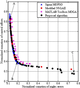
period T is 7; the swarm size and the maximum iteration are 50 and 100, respectively. The Pareto front of this multi-objective problem is shown in Fig. 2. Also, the feasibility and the efficiency of the proposed multi-objective algorithm is assessed in comparison with Sigma method [16], modified NSGAII [32] and MATLAB (R2010a) Toolbox MOGA. Although the performances of these algorithms are competitively good over this problem, the most interesting result is that the proposed algorithm has more uniformity and diversity.

In Fig. 2, points A and C stand for the best normalized summation of angles errors and normalized summation of control efforts, respectively. It is clear from this figure that all the optimum design points in the Pareto front are non-dominated and could be chosen by a designer as optimum

0.1 0.2 0.3 0.4 0.5 0.6 0.7 0.8

0.2 0.3 0.4 0.5 0.6 0.7 0.8 0.9 1

Normalized sumation of angles errors

N

or

m

al

iz

ed s

um

at

ion of

c

ont

rol

e

ffor

ts

Sigma MOPSO Modified NSGAII MATLAB Toolbox MOGA Proposed algorithm A

B

C

Fig. 2. The obtained Pareto fronts by using Sigma method [16], modified NSGAII [32], MATLAB (R2010a) Toolbox MOGA and the proposed algorithm for optimal control design of the

walking robot

Table 4. Objective functions and their associated design variables for the optimum points in Fig. 2

C B

A Optimum design point

1 7.58 10_× −

1 1.93 10_× −

1 1.22 10_× −

Normalized summation of angles errors

1 2.75 10_× −

1

3.96 10_× −

1 8.29 10_× −

Normalized summation of control efforts

2 9.34 10× 2

9.71 10× 2

9.98 10× Design variable w1

1

7.59 10× 1

9.99 10× 1

9.66 10× Design variable w₂

2

2.55 10× 2

1.84 10× 2

8.51 10× Design variable w₃

1

3.96 10× 1

5.47 10× 1

9.89 10× Design variable w₄

2

1.07 10× 2

9.67 10× 2

9.75 10× Design variable w5

1

1.04 10× 1

8.83 10× 1

fuzzy tracking controllers. It is also clear that choosing a better value for any objective function in the Pareto front would cause a worse value for another objective. the corresponding values of those objective functions show an undesirable situation in comparison with the Pareto front. This implies that if any other set of decision variables is chosen, the corresponding values of the pair of those objective functions will locate a point inferior to that Pareto front. Such inferior area in the space of the two objectives is located in fact on the

top right side of Fig. 2.

Clearly, there are some important optimal design facts between these two objective functions which have been discovered by the Pareto optimum design approach. Such important design facts could not have been found without the use of multi-objective Pareto optimization process. From Fig. 2, point B demonstrates such important optimal design fact. Point B could be the trade-off optimum choice when considering minimum values of both the normalized summation of angles

0 0.5 1 1.5 2 2.5 3 3.5 4 -100

-80 -60 -40 -20 0 20

Time (s)

C

on

tro

l E

ffo

rt u3

(N

.m

)

Optimum design point A Optimum design point B Optimum design point C

Fig. 8. Control effort u3 for the optimum design points A, B, and C shown in the Pareto front

0 0.5 1 1.5 2 2.5 3 3.5 4 -100

-80 -60 -40 -20 0 20

Time (s)

C

on

tro

l E

ffo

rt u2

(N

.m

)

Optimum design point A Optimum design point B Optimum design point C

Fig. 7. Control effort u₂ of the optimum design points A, B, and C shown in the Pareto front

0 0.5 1 1.5 2 2.5 3 3.5 4 -350

-300 -250 -200 -150 -100 -50 0 50

Time (s)

C

on

tro

E

ffo

rt u1

(N

.m

)

Optimum design point A Optimum design point B Optimum design point C

Fig. 6. Control effort u₁ for the optimum design points A, B, and C shown in the Pareto front

0 0.5 1 1.5 2 2.5 3 3.5 4 2

2.2 2.4 2.6 2.8 3 3.2 3.4

Time (s)

θ3

(ra

d)

Optimum design point A Optimum design point B Optimum design point C Desired trajectory

Fig. 5. Tracking trajectory θ3 for the optimum design points A, B, and C shown in the Pareto front

0 0.5 1 1.5 2 2.5 3 3.5 4 0.02

0.04 0.06 0.08 0.1 0.12 0.14 0.16 0.18 0.2 0.22

Time (s)

θ (ra2

d)

Optimum design point A Optimum design point B Optimum design point C Desired trajectory

Fig. 4. Tracking trajectory θ2 for the optimum design points A, B, and C shown in the Pareto front

0 0.5 1 1.5 2 2.5 3 3.5 4 -0.2

-0.18 -0.16 -0.14 -0.12 -0.1 -0.08 -0.06 -0.04 -0.02 0

Time (s)

θ1

(ra

d)

Optimum design point A Optimum design point B Optimum design point C Desired trajectory

Fig. 3. Tracking trajectory θ₁ for the optimum design points A, B, and C shown in the Pareto front

3.4 3.45 3.5 3.55 3.6 -0.135

errors and normalized summation of control efforts. Design variables and objective functions corresponding to the optimum design points A, B, and C are illustrated in Table 4. The real tracking trajectory of the optimum design points A, B, and C are shown in Figs. 3 to 5. The control effort of the optimum design points A, B, and C are also shown in Figs. 6 to 8.

7- Conclusion

This paper presented fuzzy tracking control for a walking robot that stepped purely in the lateral plane of a slope. Fuzzy control was utilized as an effective control to satisfy criteria for nonlinearity of dynamic equation and tracking system. An innovative multi-objective PSO algorithm was used to obtain the Pareto front of the non-commensurable objective functions in the design of fuzzy tracking controller. In the multi-objective optimization method, firstly, PSO was combined with convergence and divergence operators to modify converging process and also to skip every possible local optimum. Then, the periodic multi-objective optimization helped particles explore more areas in the solution space. Two conflicting objective functions, namely the normalized summation of angles errors and normalized summation of control efforts, were utilized for optimal control design. The Pareto front of innovative PSO was compared with the Pareto front of three renowned algorithms, namely modified NSGAII, Sigma method and MATLAB Toolbox MOGA. The Pareto front of innovative PSO was much more scattered than the other three and the points spread along adjacent axes. Therefore, the designer has the ample opportunity to select the finest point. Three points of Pareto front obtained from the innovative PSO were selected and the related design variables were used to illustrate the time responses of the system states. The result illustrated that the first selected point had minimum normalized summation of angles errors and maximum normalized summation of control efforts. However, the third point was opposite to the first one. It had maximum normalized summation of angles errors and minimum normalized summation of control efforts. The second well-chosen point could be the trade-off optimum choice.

Reference

[1] Z. Liu, Y. Zhang, Y.J.I.T.o.S. Wang, Man,, P.C. Cybernetics, A type-2 fuzzy switching control system for biped robots, 37(6) (2007) 1202-1213.

[2] T.-H.S. Li, Y.-T. Su, S.-W. Lai, J.-J.J.I.T.o.S. Hu, Man,, P.B. Cybernetics, Walking motion generation, synthesis, and control for biped robot by using PGRL, LPI, and fuzzy logic, 41(3) (2011) 736-748.

[3] G. Dip, V. Prahlad, P.D.J.R. Kien, Genetic algorithm-based optimal bipedal walking gait synthesis considering tradeoff between stability margin and speed, 27(3) (2009) 355-365.

[4] P.N. Mousavi, C. Nataraj, A. Bagheri, M.A.J.A.M.M. Entezari, Mathematical simulation of combined trajectory paths of a seven link biped robot, 32(7) (2008) 1445-1462.

[5] S. Ito, S. Amano, M. Sasaki, P. Kulvanitt, In-place lateral stepping motion of biped robot adapting to slope change, in: 2007 IEEE International Conference on Systems, Man and Cybernetics, IEEE, 2007, pp. 1274-1279.

[6] M.T. Khorsandi, B. Miripour-Fard, A. Bagheri, Optimal tracking control of a biped robot walking in the lateral plane, in: 2011 International Symposium on Innovations in Intelligent Systems and Applications, IEEE, 2011, pp. 560-564.

[7] D.A. Shook, P.N. Roschke, P.-Y. Lin, C.-H.J.E.s. Loh, GA-optimized fuzzy logic control of a large-scale building for seismic loads, 30(2) (2008) 436-449.

[8] H. Shayeghi, A. Jalili, H.J.E.C. Shayanfar, Management, Multi-stage fuzzy load frequency control using PSO, 49(10) (2008) 2570-2580.

[9] Z. Bingül, O.J.E.S.w.A. Karahan, A Fuzzy Logic Controller tuned with PSO for 2 DOF robot trajectory control, 38(1) (2011) 1017-1031.

[10] R. Eberhart, J. Kennedy, Particle swarm optimization, in: Proceedings of the IEEE international conference on neural networks, Citeseer, 1995, pp. 1942-1948.

[11] P.J. Angeline, Using selection to improve particle swarm optimization, in: 1998 IEEE International Conference on Evolutionary Computation Proceedings. IEEE World Congress on Computational Intelligence (Cat. No. 98TH8360), IEEE, 1998, pp. 84-89.

[12] R.C. Eberhart, Y. Shi, Comparison between genetic algorithms and particle swarm optimization, in: International conference on evolutionary programming, Springer, 1998, pp. 611-616.

[13] H. Yoshida, K. Kawata, Y. Fukuyama, S. Takayama, Y.J.I.T.o.p.s. Nakanishi, A particle swarm optimization for reactive power and voltage control considering voltage security assessment, 15(4) (2000) 1232-1239. [14] X. Hu, R. Eberhart, Multiobjective optimization using

dynamic neighborhood particle swarm optimization, in: Proceedings of the 2002 Congress on Evolutionary Computation. CEC’02 (Cat. No. 02TH8600), Ieee, 2002, pp. 1677-1681.

[15] J.E. Fieldsend, S. Singh, A multi-objective algorithm based upon particle swarm optimisation, an efficient data structure and turbulence, (2002).

[16] S. Mostaghim, J. Teich, Strategies for finding good local guides in multi-objective particle swarm optimization (MOPSO), in: Proceedings of the 2003 IEEE Swarm Intelligence Symposium. SIS’03 (Cat. No. 03EX706), IEEE, 2003, pp. 26-33.

[17] K.E. Parsopoulos, D.K. Tasoulis, M.N. Vrahatis, Multiobjective optimization using parallel vector evaluated particle swarm optimization, in: Proceedings of the IASTED international conference on artificial intelligence and applications, Acta Press, 2004, pp. 823-828.

[18] D.A. Winter, Biomechanics and motor control of human movement, John Wiley & Sons, 2009.

[19] L.-X. Wang, L.-X. Wang, A course in fuzzy systems and control, Prentice Hall PTR Upper Saddle River, NJ, 1997.

[20] R. Eberhart, P. Simpson, R. Dobbins, Computational intelligence PC tools, Academic Press Professional, Inc., 1996.

Swarm Intelligence, John Wiley \&\#38; Sons, Inc., 2006.

[22] A. Ratnaweera, S.K. Halgamuge, H.C.J.I.T.o.e.c. Watson, Self-organizing hierarchical particle swarm optimizer with time-varying acceleration coefficients, 8(3) (2004) 240-255.

[23] M.J. Mahmoodabadi, A. Bagheri, S.A. Mostaghim, M.J.M. Bisheban, C. Modelling, Simulation of stability using Java application for Pareto design of controllers based on a new multi-objective particle swarm optimization, 54(5-6) (2011) 1584-1607.

[24] M. Mahmoodabadi, A. Bagheri, N. Nariman-Zadeh, A.J.E.O. Jamali, A new optimization algorithm based on a combination of particle swarm optimization, convergence and divergence operators for single-objective and multi-objective problems, 44(10) (2012) 1167-1186.

[25] J.-J. Liang, P.N. Suganthan, Dynamic multi-swarm particle swarm optimizer, in: Proceedings 2005 IEEE Swarm Intelligence Symposium, 2005. SIS 2005., IEEE, 2005, pp. 124-129.

[26] Z.-H. Zhan, J. Zhang, Y. Li, H.S.-H.J.I.T.o.S. Chung, Man,, P.B. Cybernetics, Adaptive particle swarm optimization, 39(6) (2009) 1362-1381.

[27] J.J. Durillo, J. García-Nieto, A.J. Nebro, C.A.C. Coello, F. Luna, E. Alba, Multi-objective particle swarm optimizers: An experimental comparison, in: International conference on evolutionary multi-criterion optimization, Springer, 2009, pp. 495-509.

[28] M. Reyes-Sierra, C.C.J.I.j.o.c.i.r. Coello, Multi-objective particle swarm optimizers: A survey of the state-of-the-art, 2(3) (2006) 287-308.

[29] K. Deb, S. Agrawal, A. Pratap, T. Meyarivan, A fast elitist non-dominated sorting genetic algorithm for multi-objective optimization: NSGA-II, in: International conference on parallel problem solving from nature, Springer, 2000, pp. 849-858.

[30] R.J.J.o.p.c. Toscano, A simple robust PI/PID controller design via numerical optimization approach, 15(1) (2005) 81-88.

[31] F. Golnaraghi, B.C. Kuo, Automatic Control Systems, Wiley Publishing, 2009.

[32] K. Atashkari, N. Nariman-Zadeh, M. Gölcü, A. Khalkhali, A.J.E.C. Jamali, Management, Modelling and multi-objective optimization of a variable valve-timing spark-ignition engine using polynomial neural networks and evolutionary algorithms, 48(3) (2007) 1029-1041.

Pleasecitethisarticleusing: