Volume 19 - Article 31 | Pages 1205–1216

Demographic Researcha free, expedited, online journal of peer-reviewed research and commentary

in the population sciences published by the Max Planck Institute for Demographic Research Konrad-Zuse Str. 1, D-18057 Rostock·GERMANY www.demographic-research.org

DEMOGRAPHIC RESEARCH

VOLUME 19, ARTICLE 31, PAGES 1205-1216

PUBLISHED 11 JULY 2008

http://www.demographic-research.org/Volumes/Vol19/31/ DOI: 10.4054/DemRes.2008.19.31

Reflexion

Biological and sociological interpretations of

age-adjustment in studies of higher order birth

rates

Mette Gerster

Niels Keiding

c

°2008 Gerster & Keiding.

1 Introduction 1206

1.1 Several possible time origins 1208

2 Britta Hoem’s idea 1208

2.1 The two models 1208

2.2 How do the two models correspond? 1209

3 A simulation study 1210

3.1 The scenario 1211

3.2 Results 1213

3.3 Conclusion based on the simulation study 1213

4 Conclusion 1213

5 Acknowledgements 1214

References 1215

reflexion

Biological and sociological interpretations of age-adjustment in

studies of higher order birth rates

Mette Gerster1

Niels Keiding2

Abstract

Several studies of the effect of education on second or third birth rates (e.g Hoem et al. 2001) have used the concept ofrelative age at previous birth(Hoem 1996). B. Hoem’s idea was to focus on the social meaning of age at previous birth by redefining it accord-ing to the woman’s educational attainment. We broaden the discussion by consideraccord-ing other interpretations of the explanatory power of the age at previous birth, particularly via known trends in biological fecundity. A mathematical analysis of the approach reveals side effects that have not been taken sufficiently into account. Our recommendation is not to use the relative age approach without supplementing it with the more traditional approach which includes the actual age at previous birth.

1. Introduction

In recent years, several studies of the effect of education on second or third birth rates (Hoem et al. 2001; Oláh 2003; Kreyenfeld 2002; Köppen 2006) have used the concept ofrelative age at second (or first) birthwhich was originally introduced by Britta Hoem (1996).

The idea is that when comparing the third (second) birth rate between mothers with different education levels but the same age at second (first) birth, one does not take into account the different “social meanings” of the woman’s age at her previous birth. Hoem (1996) suggested that in order to take this problem into account one could include the age relative to the educational level of the mother at her previous birth instead of her actual (biological) age at previous birth. She made the point that"it is important to account for the very different distributions of age at second birth that women have at different educational levels, otherwise incorrect conclusions may be drawn from the analysis".

With this note we wish to clarify from a more formal (i.e. mathematical) point of view what is going on in regression models where this suggestion is employed. But first of all, let us put forward some arguments why it is important to take age into account when modeling the effect of education on fertility3_.

There are obvious biological reasons why age should be taken into account when mod-eling fertility, because age can be seen as a proxy for the woman’s biological fecundity which indeed becomes smaller with age. However, as well as a biological component, fertility also has an important behavioural component. This perspective is emphasized in Hoem’s approach, as we will argue later on.

Kreyenfeld (2002) made the point that some of the effect of education on fertility might be transmitted through a later age at previous birth because women who have a higher education become mothers later than other women. She also noted that “given that the positive effect of women’s educational attainment was primarily transmitted through a late age at first birth, it should disappear if one holds the age at first birth constant”. Köppen (2006) argued similarly that “education influences fertility alsoindirectly”. This was in fact what Hoem (1996) was aiming at: that age at previous birth is anintermediary variable between education and the birth rate that we are modeling.

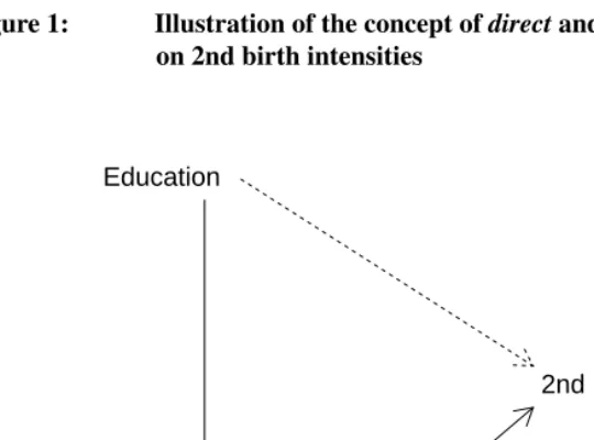
An illustration is shown in Figure 1. The broken arrow represents the so-calleddirect effectof education on fertility whereas the two solid arrows represent theindirect effectof education on fertility, i.e. the effect that ismediatedthrough the woman’s age at previous

3_{In the remainder of this paper we will focus on the effect of education and age at first birth on the second}

birth. The sum (in the linear case) of the direct and the indirect effect is referred to as the total effect4_.

The tradition in the epidemiological literature is that an intermediate variable (such as age at first birth in our example) should not be taken into account (see eg. Chapters 8 and 21 of Rothman and Greenland (1998) and Chapter 12 of Diggle et al. (2001)) since thisblocksthe part of the effect of the variable of interest which is mediated through the intermediate variable. Therefore, conditioning on the intermediate variable will result in an estimate of only the direct effect and not the total effect.

In the example where the outcome is the second-birth intensity, this corresponds to the indirect effect of education being blocked if age at previous birth is included in a regression model. Hence, the scenario indicated by Kreyenfeld corresponds to the direct effect of education on fertility being0.

Figure 1: Illustration of the concept ofdirectandindirecteffect of education on 2nd birth intensities

Education

2nd birth intensity

Age at 1st birth

4_{A diagram like the one shown in Figure 1 is referred to as adirected acyclic graph (DAG). See eg. Chapter}

1.1 Several possible time origins

Let us return to the possibilities of how to take age into account: in this kind of studies we are operating with several time origins. First, there is the time since previous birth,

t. Next, there is the already mentioned age at previous birth,a0, and finally, there is the

woman’s current age,a. These three variables are linked through the identity:a−t=a0

and in the linear case it is therefore impossible to identify the effect of each one of them. A further time dimension that could be taken into account is time since finishing education, see Kantorová (2004).

In demographic studies on the effect of education on higher order birth rates the tra-dition has been to usetas the basic time variable and include age represented by either

a0 or by therelative age at previous birthas suggested by Hoem (1996). However, for

similar reasons as those mentioned above, it is not possible to identify the linear effect of botht,a0and the relative age and also in this case a choice must be made.

2. Britta Hoem’s idea

Britta Hoem’s alternative suggestion on how to include age was based on the fact that the age at previous birth can differ considerably between women with different educational attainments (possibly due to a later entry into motherhood for highly educated women). This is exactly the mechanism that makes age at first birth intermediate between education and second birth, cf. Figure 1.

In the following, we will describe the idea introduced by Britta Hoem in mathematical terms and discuss the different interpretations that arise due to the different approaches.

2.1 The two models

For illustrative purposes we assume a very simple model in which the (logarithm of the) second-birth intensity for theith woman,λi, is independent of t. We assume that the intensity depends on education,ui, which can take the two valuesui= 0(low education) andui= 1(high education). Furthermore, we assume that age at first birth,ai, enters the model as a continuous covariate and that there are no other covariates in the model:

logλi=α+β·ui+γ·ai, i= 1, . . . , n. (1)

Now, according to Britta Hoem’s suggestion, we standardize the age variable within each educational group to obtain the relative age at first birth: Letmjbe the median age at first birth in educational groupj,j= 0,1. Therelative agecan then be written as:

ri=

½

ai−m1 ifui= 1

ai−m0 ifui= 0

and in this context Britta Hoem’s suggestion corresponds to replacing Model (1) with the model

logλi= ˜α+ ˜β·ui+ ˜γ·ri, i= 1, . . . , n. (2)

Here,exp( ˜β)is the rate ratio of a woman in educational group 1 compared to a woman in educational group 0 for a givenrelative ageat first birth. For example, ifri=rj= 0, we are comparing two women who arem1 andm0years old at first birth, respectively.

In any case, we are comparing women where the one with a high education ism1−m0

years older at first birth than the one with a low education.

This approach puts focus on thesocial meaningof age at first birth as stated by Britta Hoem.

2.2 How do the two models correspond?

In the simple (linear) mathematical setting in which we have described Britta Hoem’s idea, it can easily be shown5 _{that Model (2) is in fact just a reparametrization of Model}

(1). This simply means that if we know the parametersα,βandγin Model (1) and the median ages in the two educational groups, then we can directly calculate the parameters in Model (2) and vice versa. The formulas forβ˜andγ˜are the following:

˜

β=β+γ·(m1−m0),

˜ γ=γ.

Hence, the effect of increasing the relative age with one year is the same as the effect of increasing the absolute age with one year (γ = ˜γ). On the other hand, the effect of education changes from Model 1 to Model 2. For example, it can be seen that whenever there is a negative effect of age at first birth (γ <0), a positive effect of education (β >0) and an older age at second birth in the group with the highest education compared to the group with the lower education (m1> m0) we getβ >β˜, i.e. the effect of education will

be smaller in Model (2) than in Model (1).

The important thing is that no matter for what reason we see a positive effect of edu-cation in Model (1) (the reason could for instance be selection but it could also be an income effect), the effect of education will be smaller when relative age is included in-stead of absolute age as long as the abovemathematicalconditions (β > 0,γ <0 and

m1> m0) are present. Also note, that the difference betweenβandβ˜becomes larger the

larger the difference between the median ages in the two groups.

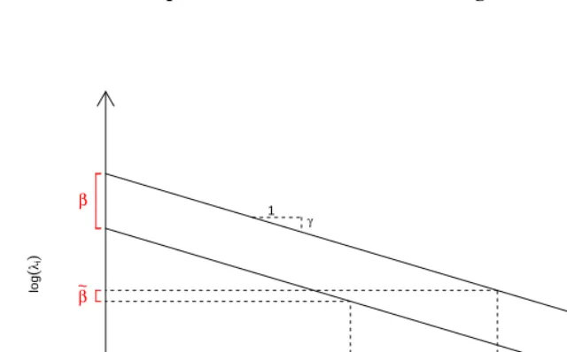
Illustration Figure 2 shows an illustration of how one can calculate the education pa-rameter,β˜, in Model (2) directly from the parameters in Model (1). The graph in Figure 2 shows the above mentioned case whereβ >0,γ <0andm1> m0. The horizontal axis

displays the age at first birth and the vertical axis thelog-intensity obtained from Model 1. Hence, the upper line corresponds to thelog-intensity for the highly educated (ui= 1), whereas the lower line corresponds to thelog-intensity for women with low education (ui = 0) as a function of age at first birth. The vertical distance between the two lines is thusβand the slope of both lines isγ. Now, assume that womanihas a low education,

ui = 0, and that womanjhas a high education,uj = 1, and that they both have an age at first birth corresponding to the median age in the two education groups,m0andm1,

respectively. Note that these two women are excactly those that we are comparing when using Model (2).

Theirlog-intensities according to Model (1) are as follows:

logλi =α+γ·m0,

logλj =α+β+γ·m1.

This gives alog-rate ratio when comparing the two women of

log µ

λj

λi

¶

= logλj−logλi=β+γ·(m1−m0) = ˜β.

It can be immediately read off from the vertical axis of the graph in Figure 2. Hence, in this simple linear case it is not even necessary to fit Model (2) in order to find the effect of education from it.

3. A simulation study

Figure 2: Graph showing how the parameter for education,β˜, from the model including relative age at first birth can be found from the parameters of the model including absolute age at first birth

age at first birth

log

(

λi

)

ui=1

ui=0

m0 m1

β

β

~

1 γ

the one model corresponds to the parameters from the other. However, the conclusion remains the same, which we will show by employing a simulation study.

3.1 The scenario

a standard error of4)6_{. The second birth intensity is assumed to be}

log(λi|(ai, ui)) = log(1/3)−0.1·max(ai−25,0),

i.e. there is a constant intensity of having the second child of1/3for women who give birth to their first child before the age of25, after this age the log-intensity decreases with0.1per additional year of age at first birth7_{. Note that there is no direct effect of}

education on the second birth intensity,β = 0. The negative effect of age on the second birth intensity could be thought of as a biological effect.

In terms of the DAG in Figure 1 this corresponds to an arrow from education to age at first birth and an arrow from age at first birth to second birth but no arrow from education to the second birth. Hence, the only effect of education on the second birth intensity is the indirect effect, i.e. the effect that is mediated through age at first birth. This means that when a model for the second-birth intensity is fitted including age at first birth and education as covariates there should be no effect of education.

We simulate this scenario 1000times with1000women in each sample. For each run we fit two Cox models8_{: one with age at first birth entering as a grouped variable}

(defined according to the observed quintiles in each run)9_{and one where the same is done}

apart from age at first birth being replaced by relative age at first birth10_{. In both cases,}

education enters the model as a categorical variable. If age at first birth exceeds40the woman is not included in the analysis of second birth. If the sum of age at first birth and the second waiting time exceeds40the second waiting time enters as a censored observation in the Cox model. The latter case corresponds to women who have one child by the age of40.

6_{We samplea}

ias15 +Wi, whereWiis drawn from aΓ-distribution with shape parameter4and scale

parameter2in the caseui = 0(corresponding to a theoretical median age at first birth of≈22.3) and

from aΓ-distribution with shape parameter4and scale parameter3in the caseui= 1(corresponding to

a theoretical median age at first birth of≈26.0).

7_{This effect of age at first birth is also rather simplified, however, it fits quite well with the marginal effect}

of age at first birth found by Gerster et al. (2007).

8_{For details on the Cox model see e.g. Therneau and Grambsch (2000).}

9_{Note that the Cox model where age enters as a grouped variable does not fit the data as we have simulated}

them. However, it fits well with how theses studies are often carried out.

10_{Hence, when fitting the Cox models we are pretending not to know the "true" underlying mechanism on}

3.2 Results

The results are as follows:

• The median age at first birth in observations withui = 0is on average (over the 1000 runs) 22.3 years whereas the corresponding number for observations with

ui= 1is25.8years.

• From the Cox model with absolute age at first birth entering as a categorical vari-able:

– The average effect of education over the1000runs isβˆ=−0.011.

– The number of times that the hypothesis of no effect of education is rejected11

at the 5%level is5.4%of the1000runs (which is approximately what we would expect).

• From the Cox model with relative age at first birth entering as a categorical variable: – The average effect of education over the1000runs is−0.135.

– The number of times that the hypothesis of no effect of education is rejected at the5%level is52%out of the1000runs.

3.3 Conclusion based on the simulation study

This simulation study was constructed to demonstrate how the effect of education changes when replacing Model (1) with Model (2) in the case where the effect of age at first birth on the second birth intensity is not linear throughout the reproductive age span (but still negative after a certain age). The data were simulated from a model in which there was no effect of education on the second birth but a negative effect on the age at first birth in the sense that women with a high education were approximately3.5years older at the time of first birth than other women. When age at first birth was controlled for in the model for the second birth intensity there was no effect of education, but when it was controlled for in terms of relative age there was a negative effect of education which was significantly different from0in approximately half of the runs.

4. Conclusion

Hoem (1996) focused on the conceptual content in taking into account the age at previous birth, arguing that the social meaning might be emphasized by including the relative age at birth of the previous child instead of the absolute age at birth of the previous child. Employing Britta Hoem’s suggestion indeed changes the interpretation of the education effect towards a more social perspective because the comparison is no longer between two women of the same biological age but between two women of the same relative (social)

age as we have discussed above. This can be a valid focus to have in mind in these kind of studies.

Furthermore, Hoem’s paper points to the fact that age at previous birth might be an intermediate variable on the pathway between education and a given higher order birth rate as illustrated in Figure 1. Also this point is very relevant since some studies have shown a postponement pattern among women with a higher education, cf. eg. Lappegård and Rønsen (2005).

However, there are implications of using this approach that should be kept in mind, and our recommendation would be not to use Hoem’s approach without supplementing it with the more traditional approach. This is due to the fact that, as we have shown in the above, in the case when there is a negative effect of age at first birth on the second birth intensity and the only effect of education is the one mediated through age at previous birth (possibly due to the mentioned postponement mechanism), the negative age effect will show up as a negative effect of education in the model including relative age, and this will be the case solely due to the fact that the comparison is between women of a different age.

Also, there is another issue that we have completely ignored so far: in many studies the available data on education are updated eg. each year throughout the study period, in which case education can (and should) be included as a time-varying covariate. But then it is not clear how relative age at first birth should be defined12_{and the interpretation}

of the effect of a time-varying education variable when age at first birth is included as relative age in this manner becomes very unclear.

Finally, as we have discussed with the DAG in Figure 1 as point of reference, the education influences the age at first birth, but there might well be substantive basis for an arrow pointing in the opposite direction as well, i.e. there are feedback mechanisms between education and fertility which are not considered. This gives rise to the question which has also been raised by eg. Kravdal (2001, 2007) that focusing on one parity tran-sition when studying the effect of education on fertility might be a too simple approach.

5. Acknowledgements

We are grateful to Jan M. Hoem for several discussions on this topic and to Esben Budtz-Jørgensen for a useful suggestion regarding Figure 2. Furthermore, we would like to thank two anomymous reviewers for valuable comments on an earlier draft of the paper.

References

Diggle, P. J., Liang, K.-Y., and Zeger, S. L. (2001).Analysis of Longitudinal Data. Oxford Statistical Science Series. Oxford Univerity Press, Oxford. second edition.

Gerster, M., Keiding, N., Knudsen, L., and Strandberg-Larsen, K. (2007). Education and second birth rates in Denmark, 1981-1994.Demographic Research, 17:181–210. Hoem, B. (1996). The social meaning of the age at second birth for third-birth fertility:

A methodological note on the need to sometimes respecify an intermediate variable. Yearbook of Population Research in Finland, 33:333–339.

Hoem, J., Prskawetz, A., and Neyer, G. (2001). Autonomy or conservative adjustment? the effect of public policies and educational attainment on third births in Austria, 1975-96.Population Studies, 55(3):249–261.

Kantorová, V. (2004). Education and entry into motherhood: The Czech Republic during state socialism and the transition period (1970-1997).Demographic Research, S3:245– 274.

Köppen, K. (2006). Second births in western Germany and France. Demographic Re-search, 14:295–330.

Kravdal, Ø. (2001). The high fertility of college educated women in Norway. Demo-graphic Research, 5:187–215.

Kravdal, Ø. (2007). Effects of current education on second- and third-birth rates among Norwegian women and men born in 1964: Substantive interpretations and methodolog-ical issues.Demographic Research, 17:211–246.

Kreyenfeld, M. (2002). Time-squeeze, partner effect or self-selection? An investigation into the positive effect of women’s education on second birth risks in Western Germany. Demographic Research, 7:15–48.

Lappegård, T. and Rønsen, M. (2005). The multifaceted impact of education on entry into motherhood.European Journal of Population, 21(1):31–49.

Oláh, L. (2003). Gendering fertility: Second births in Sweden and Hungary. Population Research and Policy Review, 22(2):171–200.

Pearl, J. (2001). Direct and indirect effects. Proceedings of the Seventeenth Conference on Uncertainty in Artificial Intelligence. pages 411–420.

Rothman, K. and Greenland, S. (1998). Modern Epidemiology. Lippincott-Raven, Philadelphia. 2 edition.

Appendix

Calculations showing the connection between the models

Model 1:

logλi=α+β·ui+γ·ai, i= 1, . . . , n,

whereui∈ {0,1}andai>0. Letm1be the median age at second birth andσ12the

vari-ance of age at second birth among women withui= 1and definem0andσ20accordingly

for women withui= 0.

Model 2:

logλi= ˜α+ ˜β·ui+ ˜γ·ri, i= 1, . . . , n,

whererirepresents the so-calledrelative age at second birth13, which in this case corre-sponds tori= (ai−m1)/σ1ifui= 1andri = (ai−m0)/σ0ifui= 0.

In the following we go through the parameters in each of the two models to show how they correspond to each other.

From the two models we get that

α+β·ui+γ·ai= ˜α+ ˜β·ui+ ˜γ·ri. Plugging inui= 0,ai=m0gives

˜

α=α+γ·m0.

Puttingu1= 1andai=m1and applying the above formula forα˜gives

α+β+γ·m1=˜α+ ˜β

=α+γ·m0+ ˜β

⇓

˜

β =β+γ·(m1−m0).

Finally, plugging inui= 0andri = 1(⇒ai =σ0+m0), this implies that

α+γ·(σ0+m0) =˜α+ ˜γ

=α+γm0+ ˜γ

⇒ γ˜=γ·σ0.

13_{In the above calculations the definition of relative age is allowed to depend on the possibly different standard}

errors,σ0 andσ1, in the age distributions within the two educational groups. However, since this has no