Numerical solution of the forced Duffing equations using Legendre
multiwavelets
Ramin Najafi∗
Department of Mathematics,
Maku Branch, Islamic Azad University, Maku, Iran.
E-mail: r−[email protected]
Behzad Nemati Saray Faculty of Mathematics,
Institute for Advanced Studies in Basic Sciences, Zanjan, Iran.
E-mail: [email protected]
Abstract A numerical technique based on the collocation method using Legendre multiwavelets are presented for the solution of forced Duffing equation. The operational matrix of integration for Legendre multiwavelets is presented and is utilized to reduce the solution of Duffing equation to the solution of linear algebraic equations. Illustra-tive examples are included to demonstrate the validity and applicability of the new technique.
Keywords. Forced Duffing equations, Multiwavelet, Operational matrix of integration, Collocation method.
2010 Mathematics Subject Classification. 65M70, 65T60, 49J20.
1. Introduction
In this paper, we consider the following forced Duffing equation [4]
u′′(t) +σu′(t) +f(t, u) = 0, 0< t <1, σ∈R−0, (1.1)
with integral boundary conditions
µ1u(0)−µ2u′(0) =
∫1
0 h1(s)u(s)ds,
µ3u(1)−µ4u′(1) =
∫1
0 h2(s)u(s)ds,
(1.2)
wheref : [0,1]×R→R andµi are nonnegative constant.
The Duffing equation is a well known nonlinear equation of applied science which is used as a powerful tools to discuss some important practical phenomena such as orbit extraction, nonuniformity caused by an infinite domain, nonlinear mechanical oscillators, ets. An important application of the Duffing equation is in the field of the prediction of diseases. The numerical solutions of the forced Duffing equations with two-point boundary conditions have been widely investigated [18,21,24]. How-ever, there are few references on the forced Duffing equation with integral boundary conditions [19].
Received: 12 December 2016 ; Accepted: 28 February 2017.
∗Corresponding author.
The existence and uniqueness of the solution of the forced Duffing equation with integral boundary conditions are presented by means of a constructive method [6]. Dehghan presented some effective methods for solving problems with nonlocal condi-tions [12–17].
Wavelets theory is a relatively new and emerging area in mathematical research. It has been applied in a wide range of engineering disciplines; in particular, wavelets are very successfully used in signal analysis for waveform representation and segmen-tations, time-frequency analysis and fast algorithms for easy implementation [8,9].
Wavelets permit the accurate representation of a variety of functions and operators. Moreover wavelets establish a connection with fast numerical algorithms [5]. Publi-cations on integral equation methods have shown a marked preference for orthogonal wavelets [22].
Different variations of wavelet bases (orthogonal, biorthogonal, multiwavelets) have been presented and the design of the corresponding wavelet and scaling functions has been addressed [7,10,11,20]. Multiwavelets are generated by more than one scaling function [1,20]. Multiwavelets have some advantages in comparison to single wavelets. For example, such features as short support, orthogonality, symmetry and vanishing moments are known to be important in signal processing and numerical methods. A single wavelets cannot possess all these properties at the same time. On the other hand, a multiwavelets system can have all of them simultaneously [25]. This suggests that multiwavelets could perform better in various applications.
In this paper, we use Legendre (Alpert) multiwavelets for solving forced Duffing equation with integral boundary conditions. These multiwavelets constructed in [1] and also considered in [2] and [3]. Our method consists of reducing forced Duffing equation equation to a set of algebraic equations by expanding unknown function as Legendre multiwavelets with unknown coefficients. The properties of these multi-wavelets are then utilized to evaluate the unknown coefficients.
The paper is organized as follows: Section 2 is devoted to the basic formulation of the Legendre multiwavelets required for our subsequent development. In Section 3 the proposed method is used to approximate the Duffing equation. In Section 4, we report our numerical finding and demonstrate the accuracy of the proposed numerical scheme by considering numerical examples. Section 5, ends this paper with a brief conclusion
2. Legendre multiwavelets systems
2.1. Multiresolution analysis. For functions ϕm ∈ L2(R), m = 0, . . . , r, let a reference subspace or sample space V0 be generated as the L2-closure of the linear span of the integer translates ofϕm, namely:
V0=closL2⟨ϕm(.−k) :k∈Z⟩, m= 0, . . . , r,
and consider other subspace
Vj=closL2
⟨
ϕmj,k:k∈Z⟩, j∈Z, m= 0, . . . , r,
whereϕm j,k=ϕ
Definition 1. Functionsϕm∈L2(R), is said to generate a multiresolution analysis (MRA) if they generate a nested sequence of closed subspacesVj that satisfy
i) · · · ⊂V−1⊂V0⊂V1⊂ · · ·,
ii) closL2(∪j∈ZVj
)
=L2(R),
iii) ∩j∈ZVj = 0,
iv) f(x)∈Vj⇐⇒f(x+ 2−j)∈Vj ⇐⇒f(2x)∈Vj+1,
v) {ϕm(.−k)}k∈Z, form a Riesz basis ofV0.
(2.1)
Ifϕm generate an MRA, then ϕm are called scaling functions. In case the different
integer translate ofϕmare orthogonal (with respect to the standard inner product<
f, g >=∫−∞∞ f(x)g(x)dxfor two functions inL2(R)), denoted byϕm(.−k)⊥ϕm˜(.−k˜)
form̸= ˜m, k̸= ˜k, the scaling functions are called an orthogonal scaling functions. As the subspaces Vj are nested, there exist complementary orthogonal subspaces
Wj such that
Vj+1=Vj
⊕
Wj, j∈Z,
where⊕denotes orthogonal sums.
This give rise to an orthogonal decomposition ofL2(R), namely:
L2(R) =⊕
j∈Z
Wj.
Definition 2. Functions ψm∈L2(R) are called wavelets, if they generate the com-plementary orthogonal subspacesWj of an MRA, i.e.,
Wj =closL2 < ψj,km, k∈Z >, j∈Z, m= 0, . . . , r,
whereψm
j,k=ψm(2jx−k),j, k∈Z.
Obviously, ψmj,k⊥ψm˜˜
j,˜k for j ̸= ˜j, m ̸= ˜m and k ̸= ˜k if < 2 j/2ψm
j,k,2 ˜ j/2ψm˜
˜j,˜k >=
δj,˜jδk,˜kδm,m˜ thenψmare called orthonormal wavelets.
Now we define Legendre scaling functions and its corresponding multiwavelets ac-cording to the above MRA.
2.2. Construction of Scaling Functions. Legendre multiwavelets system with multiplicityrconsist of rscaling functions andrwavelets. The r-th order Legendre scaling functions are the set ofr+ 1 functionsϕ0(x), ..., ϕr(x) whereϕi(x) is a
polyno-mial ofi-th order and allϕ’s form orthonormal basis, that is [2,24], fori= 0,1, ..., r,
ϕi(x) =
i
∑
k=0
aikxk, fori= 0,1, ..., r. (2.2)
The coefficientsaikare chosen so that
∫ 1
0
ϕi(x)ϕk(x)dx=δi,k, fori, k= 0,1, ..., r, (2.3)
where
δi,k=
{
The scaling functionsϕi(x) foriis even, odd have symmetry, anti-symmetry prop-erties, respectively. The two scale relations for Legendre scaling functions of orderr, are in the form [2]:
ϕi(x) =
r
∑
j=0
pi,jϕj(2x) + r
∑
j=0
pi,r+j+1ϕj(2x−1), i= 0,1, . . . , r. (2.4)
The coefficients{p}are determined uniquely by substituting the equations (2.2) into (2.4). We would like to mention two remarks on the two-scale relations.
1. sinceϕi(x) is ai-thorder polynomial, the right hand side of (2.4) has at most
i-thorder scaling functions. Therefore,pi,j=pi,r+j+1= 0 for i < j.
2. The two-scale relations for the Legendre scaling function of the ordernwhich is lower thanris a subset of the firstntwo-scale relations forϕi fori= 0,1, ..., nform r-thorder two scale relations.
2.3. Construction of Wavelets. The two-scale relations for ther-th order Legendre multiwavelets are in the form [2]:
ψi(x) =
r
∑
j=0
qi,jϕj(2x) + r
∑
j=0
qi,r+j+1ϕj(2x−1). (2.5)
As we have 2(r+ 1)2 unknown coefficients {q} in (2.5), use the following 2r(r+ 1) vanishing moment conditions (2.6) and 2(r+ 1) orthonormal conditions (2.7) to determine them.
1. Vanishing moments
∫ 1
0
ψi(x)xj= 0, fori= 0,1, ..., r j= 0,1, ..., i+r. (2.6)
2. Orthonormality
∫ 1
0
ψi(x)ψj(x) =δi,j, f or i, j= 0,1, ..., r. (2.7)
For example the cubic Legendre scaling functions consist of the four functions in (2.8).
ϕ0(x) = 1, 0≤x <1,
ϕ1(x) =√3(2x−1), 0≤x <1, ϕ2(x) =√5(6x2−6x+ 1), 0≤x <1,
ϕ3(x) =√7(20x3−30x2+ 12x−1), 0≤x <1.
(2.8)
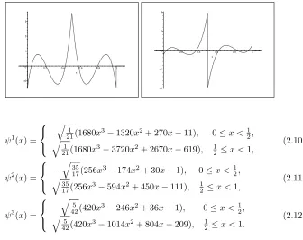
The closed form solution to the cubic Legendre multiwaveletsψ0(x),ψ1(x),ψ2(x) andψ3(x) are in (2.9)-(2.12) which are determined using the condition (2.6) and (2.7). Figures 1 and 2 show the plots of cubic Legendre multiwavelets.
ψ0(x) =
−√15 17(224x
3−216x2+ 56x−3), 0≤x < 1 2,
√
15 17(224x
3−456x2+ 296x−61), 1
2 ≤x <1,
Figure 1. The plots of cubic Legendre multiwaveletsψ0 (left), andψ1 (right).
–2 –1 0 1
0.2 0.4 0.6 0.8 1 x
–2 –1 1 2
0.2 0.4 0.6 0.8 1 x
Figure 2. The plots of cubic Legendre multiwaveletsψ2 (left), andψ3 (right).
–1 0 1 2 3
0.2 0.4 0.6 0.8 1 x
–4 –2 0 2 4
0.2 0.4 0.6 0.8 1 x
ψ1(x) =
√
1 21(1680x
3−1320x2+ 270x−11), 0≤x < 1 2,
√
1 21(1680x
3−3720x2+ 2670x−619), 1
2 ≤x <1,
(2.10)
ψ2(x) =
−√35 17(256x
3−174x2+ 30x−1), 0≤x < 1 2,
√
35 17(256x
3−594x2+ 450x−111), 1
2 ≤x <1,
(2.11)
ψ3(x) =
√
5 42(420x
3−246x2+ 36x−1), 0≤x < 1 2,
√
5 42(420x
3−1014x2+ 804x−209), 1
2 ≤x <1.
(2.12)
2.4. Function Approximation. It can be verified that Vj ⊕Wj =Vj+1, thus we can writeVj=V0⊕(⊕ij=0−1Wi) and we have two kind of basis sets forJ ∈N
ΦJ(x) =
[
ϕ0J,0(x), ..., ϕrJ,0(x),| · · ·, ϕ0J,(2J−1)(x), ..., ϕ r
J,(2J−1)(x)
]T
, (2.13)
ΨJ(x) =
[
ϕ00,0(x), ..., ϕr0,0(x),|ψ00,0(x), . . . , ψ0r,0(x)|, (2.14)
. . .|ψJ0−1,0(x), . . . , ψrJ−1,0(x)|, . . . , ψJ0−1,2J−1−1(x), . . . , ψJr−1,2J−1−1(x)
]T
Now any functionf(x) on [0,1] can be approximated using scaling functions as
f(x) = 2∑J−1
k=0 r
∑
m=0
cJ,kϕmJ,k(x) =C TΦ
J(x), (2.15)
and the corresponding wavelet functions as
f(x) =
r
∑
m=0
cm0,0ϕ
m 0,0(x) +
J∑−1
j=0 2j−1
∑
k=0
dmj,kψj,km(x)
=DTΨJ(x), (2.16)
where
cmJ,k=
∫ 1
0
f(x)ϕmJ,k(x)dx, (2.17)
dmj,k=
∫ 1
0
f(x)ψj,km(x)dx, (2.18)
andDand Care (n×1) vectors withn= (r+ 1)2J given by
D=
[
c00,0, ..., cr0,0|d00,0, ..., dr0,0|...|d0J−1,0, ..., drJ−1,0|, ..., d0J−1,2J−1−1, ...drJ−1,2J−1−1
]T
,
(2.19)
C=
[
c0J,0, ..., crJ,0|...|c0J,2J−1, ..., crJ,2J−1
]T
. (2.20)
2.5. The Operational Matrix of Integral. The integral of vectors ΨJ(x) and
ΦJ(x) can be expressed as
∫ x
0
ΨJ(t)dt=IψΨJ(x), (2.21)
∫ x
0
ΦJ(t)dt=IϕΦJ(x), (2.22)
where Iψ and Iϕ are (n×n) operational matrices of integral for Legendre scaling
functions and multiwavelets. The matrixIψ can be obtained by the following process.
Let
a0= 1, ai =
√ a2
i−1+ 2, fori= 1,2, . . . , r,
bi=
1 ai−1ai
, fori= 1,2, . . . , r,
Ar=
0 b1 0
0 b2 0
0 b3 0
. .. . .. . .. 0 br−2 0
0 br−1 0
r×r
Br=
1 2J
1 · · · 0 ..
. ...
0 · · · 0
r×r
,
Mr=
1 2J+1
(
Ar−ATr + 2JBr
) .
Now it can be shown that
Iϕ=
Mr Br · · · Br
. .. . .. ... Mr Br
0 Mr
n,n
,
whereIϕ is the operational matrix of Legendre scaling functions.
The matrixIψ can be obtained by considering
ΨJ =GΦJ+1, (2.23)
whereGis a (n×n) matrix, which can be calculated as follows. Equations (2.4) give
Φj =PjΦj+1, (2.24)
where Pj, j = 1,2, ..., J is a (r2j−1, r2j) and members of Pj are the coefficient at
(2.4).
From (2.5) we have
Ψj =QjΦj+1, (2.25)
where Qj, j = 1,2, ..., J is a (r2j−1, r2j) and members of Qj are the coefficient at
(2.5).
Using expressions (2.23), (2.24) and (2.25) we get
G=
P1×P2×...×PJ
Q1×P2×...×PJ
.. .
QJ−2×PJ−1× ×PJ
QJ−1×PJ
QJ
n×n
. (2.26)
Using expressions (2.21) (2.22) and (2.23) we have
∫ x
0
ΨJ(t)dt=G
∫ x
0
ΦJ+1(t)dt=GIϕΦJ+1(x) =GIϕG−1ΨJ(x). (2.27)
Comparing Eqs. (2.21) and (2.27) we get
3. Description of Numerical Method
In this section, we solve forcing Duffing equation of the form in (1.1), by using Legendre multiwavelets.
For this purpose, we first assume
z(t) =f(t, u(t)), . (3.1)
Using Eq. (2.16) we get
z(t) =ZTΨJ(t), (3.2)
whereZ is a (n×1) unknown vector defined similarly toDin (2.19). Let
u′′(t) =UTΨJ(t), (3.3)
by integrating from both sides of Eq.(3.3) and by using (2.21) we get
u′(t)−u′(0) =UT ∫ t
0
ΨJ(x)dx=UTIψΨJ(t), (3.4)
now we put
u′(0) =α,
thus
u′(t) =UTIΨΨJ(t) +α. (3.5)
Again by integrating from both sides of Eq. (3.5) we have
u(t)−u(0) =UTIψ2ΨJ(t) +αt. (3.6)
Suppose
u(0) =β,
so we get
u(t) =UTIψ2ΨJ(t) +αt+β. (3.7)
Using Eq. (2.19) we get
α= ΛΨJ(t). (3.8)
where Λ is a (n×1) vector as
Λ = [α,0, . . . ,0]T.
Using Eqs. (3.2)−(3.8), in Eq. (1,1), we get
UTΨJ(t) +σUTIΨΨJ(t) +σΛΨJ(t) +ZTΨJ(t) = 0,
or (
UT +σUTIΨ+σΛ +ZT
)
ΨJ(t) = 0.
So we get
UT +σUTIΨ+σΛ +ZT = 0. (3.9)
Using Eqs.(3.2) and (3.7) in Eq. (3.1) we have
Collocating Eq. (3.10) innpointsti=i/(n−1), i= 0,· · ·, n−1 we get
f(t, UTIψ2ΨJ(ti) +αti+β) =ZTΨJ(ti). (3.11)
The functionsh1(s) andh2(s) in Eq. (1.2), using Eq. (2.16) may be approximated as
h1(s) =H1TΨJ(s),
h2(s) =H2TΨJ(s),
(3.12)
whereH1 andH2 are (n×1) vectors with the entries as
(H1)i=
∫1
0 h1(s)(ΨJ)i(s)ds, (H2)i=
∫1
0 h2(s)(ΨJ)i(s)ds.
Applying Eqs. (3.5), (3.7) and (3.12) in Eq. (1.2) we get
µ1(UTIψ2ΨJ(0)+β)−µ2(UTIΨΨJ(0)+α)−UTIψ2
(∫ 1
0
ΨJ(s)ΨTJ(s)ds
) H1T
+αH1T
∫ 1
0
sΨJ(s)ds+βH1T
∫ 1
0
ΨJ(s)ds= 0, (3.13)
and
µ3(UTIψ2ΨJ(1)+α+β)−µ4(UTIΨΨJ(1)+α)−UTIψ2
(∫ 1
0
ΨJ(s)ΨTJ(s)ds
) H2T
+αH2T
∫ 1
0
sΨJ(s)ds+βH2T
∫ 1
0
ΨJ(s)ds= 0. (3.14)
The second and the third integral terms in Eqs. (3.13) and (3.14), regarding Eq. (2.6) can be calculated as
V1=
∫1
0 sΨ(s)ds= [ 1 2,
√ 3
6 ,0, . . . ,0] T,
V2=
∫1
0 Ψ(s)ds= [1,0, . . . ,0] T.
(3.15)
Using Eq.(2.7) in Eqs. (3.13) and (3.14) we get
µ1(UTIψ2ΨJ(0) +β)−µ2(UTIΨΨJ(0) +α)−UTIψ2H T 1 +αH
T
1V1+βH1TV2= 0, (3.16)
µ3(UTIψ2ΨJ(1)+α+β)−µ4(UTIΨΨJ(1)+α)−UTIψ2H T 2+αH
T
2V1+βH2TV2= 0. (3.17)
Equation (3.9),(3.11), (3.16) and (3.17) give a system of algebraic equations with (2n+ 2) equations and unknowns, which can be solved to find Uk and Zk, k =
Figure 3. Absolute errors forr= 4, J= 2 (left), andr= 3, J= 2 (right).
–1e–05 –8e–06 –6e–06 –4e–06 –2e–06 0 2e–06
0.2 0.4 0.6 0.8 1
x
–0.0002 –0.00015 –0.0001 –5e–05 0 5e–05 0.0001
0.2 0.4 x 0.6 0.8 1
4. Example
In this section we give some computational results of numerical experiments with methods based on preceding section, to support our theoretical discussion. The non-linear systems obtained by the collocation method are solved by the Newton method.
Example 1. Consider the following forced Duffing equation [19]:
{
u′′(t) +u′(t) +t(1−t)u3=f(t), 0< t <1,
u(0)− 2
π2u′(0) =−
∫1
0 u(s)ds, u(1) + 1
π2u′(1) =−
∫1
0 su(s)ds,
where
f(t) =πcos(πt)−sin(πt)(π2+ (−1 +t) sin(πt)2).
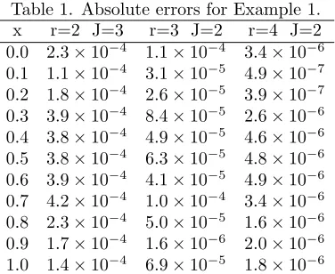
The exact solution is u(x) = sin(πt). Table 1 and Figure 3 represents the absolute values errors obtained in solving this test example with different values ofrandJ.
Table 1. Absolute errors for Example 1.
x r=2 J=3 r=3 J=2 r=4 J=2
Figure 4. Absolute errors forr= 4, J= 2 (left), andr= 4, J= 3 (right).
0 1e–05 2e–05 3e–05
0.2 0.4 0.6 0.8 1
x
–1.2e–06 –1e–06 –8e–07 –6e–07 –4e–07 –2e–07
0 0.2 0.4 0.6 0.8 1
x
Example 2. Consider the following forced Duffing equation:
u′′(t)−u′(t) +tu2=f(t), 0< t <1,
2
3πu(0) +u′(0) =−
∫1 0 sin(
πs
2)u(s)ds, 2
π2u(1) +u′(1) =
∫1
0(s+ 2)u(s)ds, wheref(t) =πsin(πt)−π2cos(πt) +tcos(πt)2. The exact solution is given by
u(x) = cos(πt).
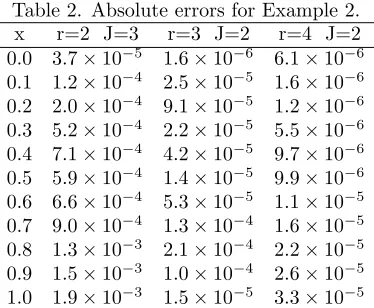
Table 2 and Figure 4 present the absolute errors for different values ofrandJ, using the present method.
Table 2. Absolute errors for Example 2.
x r=2 J=3 r=3 J=2 r=4 J=2
0.0 3.7×10⁻⁵ 1.6×10⁻⁶ 6.1×10⁻⁶ 0.1 1.2×10⁻⁴ 2.5×10⁻⁵ 1.6×10⁻⁶ 0.2 2.0×10⁻⁴ 9.1×10⁻⁵ 1.2×10⁻⁶ 0.3 5.2×10⁻⁴ 2.2×10⁻⁵ 5.5×10⁻⁶ 0.4 7.1×10⁻⁴ 4.2×10⁻⁵ 9.7×10⁻⁶ 0.5 5.9×10⁻⁴ 1.4×10⁻⁵ 9.9×10⁻⁶ 0.6 6.6×10⁻⁴ 5.3×10⁻⁵ 1.1×10⁻⁵ 0.7 9.0×10⁻⁴ 1.3×10⁻⁴ 1.6×10⁻⁵ 0.8 1.3×10⁻³ 2.1×10⁻⁴ 2.2×10⁻⁵ 0.9 1.5×10⁻³ 1.0×10⁻⁴ 2.6×10⁻⁵ 1.0 1.9×10⁻³ 1.5×10⁻⁵ 3.3×10⁻⁵
Example 3. Consider the following forced Duffing equation:
u′′(t)−2u′(t) +t2u2=f(t), 0< t <1,
u(0) +94π3u′(0) =−
∫1
0 ssin(πs)u(s)ds, u(1)− 1
2π2u′(1) =−
∫1
0(2s−1)u(s)ds, where
Figure 5. Absolute errors forr= 4, J= 2 (left), andr= 4, J= 3 (right).
–0.0003 –0.0002 –0.0001 0 0.0001 0.0002 0.0003
0.2 0.4 x 0.6 0.8 1
–1.5e–05 –1e–05 –5e–06 0 5e–06 1e–05 1.5e–05 2e–05
0.2 0.4 0.6 0.8 1
x
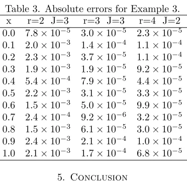
The exact solution is u(x) = sin(2πt). The absolute errors are obtained in Table 3 and Figure 5, using the presented method, for different values ofrandJ.
Table 3. Absolute errors for Example 3.
x r=2 J=3 r=3 J=3 r=4 J=2
0.0 7.8×10⁻⁵ 3.0×10⁻⁵ 2.3×10⁻⁵ 0.1 2.0×10⁻³ 1.4×10⁻⁴ 1.1×10⁻⁴ 0.2 2.3×10⁻³ 3.7×10⁻⁵ 1.1×10⁻⁴ 0.3 1.9×10⁻³ 1.9×10⁻⁵ 9.2×10⁻⁵ 0.4 5.4×10⁻⁴ 7.9×10⁻⁵ 4.4×10⁻⁵ 0.5 2.2×10⁻³ 3.1×10⁻⁵ 3.3×10⁻⁵ 0.6 1.5×10⁻³ 5.0×10⁻⁵ 9.9×10⁻⁵ 0.7 2.4×10⁻⁴ 9.2×10⁻⁶ 3.2×10⁻⁵ 0.8 1.5×10⁻³ 6.1×10⁻⁵ 3.0×10⁻⁵ 0.9 2.4×10⁻³ 2.1×10⁻⁴ 1.0×10⁻⁴ 1.0 2.1×10⁻³ 1.7×10⁻⁴ 6.8×10⁻⁵
5. Conclusion
In this article, we presented a numerical scheme for solving the forced Duffing equation with integral boundary conditions. The Legendre multiwavelets [1–3] on interval [0, 1] are employed to solve this equation. The obtained results show that this approach can solve the problem effectively.
References
[1] B. Alpert, G. Beylkin, R. Coifman, and V. Rokhlin,Wavelet-Like Bases for the Fast Solution
of Second-Kind Integral Equations, SIAM J. Sci. Comput.,14(1993), 159–184.
[2] B. Alpert, G. Beylkin, D. Gines, and L. Vozovoi, Adaptive Solution of Partial Differential
Equations in Multiwavelet Bases, J. Comput. Phys.,182(2002), 149–190.
[3] A. Averbuch, M. Israeli, and L. Vozovoi,Solution of Time Dependent Diffusion Equations with
Variable Coefficients using Multiwavelets, J. Comput. Phys.,150(1999), 394–424.
[4] S. Balaji,A new approach for solving Duffing equations involving both integral and non-integral
[5] G. Beylkin, R. Coifman, and V. Rokhlin,Fast wavelet transforms and numerical algorithms I,
Commun. Pur. Appl. Math.,44(1991), 141–83.
[6] A. Boucherif,Second order boundary value problems with integral boundary condition, Nonlinear
Anal. Theor,70(2009), 364–371.
[7] A. Cohen, I. Daubechies, and J. C. Feauveau, Biorthogonal bases of compactly supported
wavelets, Commun. Pur. Appl. Math.,45(1992), 485–560.
[8] C. K. Chui,Wavelets: A Mathematical Tool for Signal Analysis, Philadelphia, PA: SIAM, 1997.
[9] C. K. Chui,An Introduction to Wavelets, Boston: Academic 1992.
[10] I. Daubechies,Orthonormal bases of compactly supported wavelets, Commun. Pur. Appl. Math.,
41(1998), 909–996.
[11] I. Daubechies,Ten Lectures on Wavelets, CBMS-NSF Lecture Notes nr. 61, SIAM, 1992.
[12] M. Dehghan,Fully implicit finite differences methods for two-dimensional diffusion with a
non-local boundary condition, J. Comput. Appl. Math.,106(1999), 255–269.
[13] M. Dehghan, Implicit locally one-dimensional methods for two-dimensional diffusion with a
non-local boundary condition, Appl. Math. Comput.,49(1999), 331–349.
[14] M. Dehghan,Crank-Nicolson finite difference method for two-dimensional diffusion with an
integral condition, Appl. Math. Comput.,124(2001), 17–27.
[15] M. Dehghan,A new ADI technique for two-dimensional parabolic equation with an integral
condition, Comput. Math. Appl.,43(2002), 1477–1488.
[16] M. Dehghan,Numerical solution of a non-local boundary value problem with Neumann’s
bound-ary conditions, Commun. Numer. Meth. En.,19(2003), 1–12.
[17] M. Dehghan and M. Lakestani,The Use of cubic B-spline scaling functions for solving the
one-dimensional hyperbolic equation with a nonlocal conservation condition, Numer. Meth. Part. D.
E.,23(2007), 1277–1289.
[18] M. El-kady, and E. M. E. Elbarbary, A Chebyshev expansion method for solving nonlinear
optimal control problems, Appl. Math. Comput.,129(2002), 171–182.
[19] F. Geng and M. Cui,New method based on the HPM and RKHSM for solving forced Duffing
equations with integral boundary conditions, J. Comput. Appl. Math.,233(2009), 165–172.
[20] L. Herv´e,Multi-resolution analysis of multiplicity: Applications to dyadic interpolation, Appl.
Comput. Harmonic Anal.,1(1994), 299-315.
[21] M. Lakestani, M. Razzaghi, and M. Dehghan, Numerical solution of the controlled Duffing
oscillator by semi-orthogonal spline wavelets, Phys. Scr.,74(2006), 362–366.
[22] R. D. Nevels, J. C. Goswami, and H. Tehrani,Semi-orthogonal versus orthogonal wavelet basis
sets for solving integral equations, IEEE T. Antenn. Propag.,45(1997), 1332–1339.
[23] M. Shamsi and M. Razzaghi,Solution of Hallen’s integral equation using multiwavelets, Comput.
Phys. Commun.,168(2005), 187–197.
[24] M. Shamsi and M. Razzaghi, Numerical solution of the controlled Duffing oscillator by the
interpolating scaling functions, J. Electromagnet. Waves.,18(2004), 691–705.
[25] G. Strang and V. Strela,Short wavelets and matrix dilation equations, IEEE T. Signal Proces.,