in the population sciences published by the Max Planck Institute for Demographic Research Konrad-Zuse Str. 1, D-18057 Rostock · GERMANY www.demographic-research.org
DEMOGRAPHIC RESEARCH
VOLUME 9, ARTICLE 1, PAGES 1-24
PUBLISHED 29 AUGUST 2003
www.demographic-research.org/Volumes/Vol9/1/
DOI: 10.4054/DemRes.2003.9.1
Research Article
Estimating multistate transition rates
from population distributions
Robert Schoen
Stefan H. Jonsson
1 Introduction 2
2 The iterative proportional fitting method 2
3 The relative state attraction method 4 3.1 The conceptual foundation 4 3.2 Determining the adjustment factors 5
4 Evaluating the RSA method 7
4.1 Evaluations of hypothetical changes in rates 7 4.1.1 Models with two living states 7 4.1.2 Models with four living states 10 4.2 Evaluations of estimates using actual data for the
standard rates
13
5 A substantive application 15
6 Summary and conclusions 17
7 Acknowledgements 18
Notes 19
References 20
Appendix A 22
Research Article
Estimating multistate transition rates from population distributions
Robert Schoen 1
Stefan H. Jonsson2
Abstract
The ability to estimate interstate transition rates (or probabilities) from population distributions has many potential applications in demography. Iterative Proportional Fitting (IPF) has been used for such estimation, but lacks a meaningful behavioral foundation. Here a new approach, Relative State Attraction (RSA), is advanced. It assumes that states have a greater (or lesser) ability to attract individuals, and that rates respond accordingly. The RSA estimation procedure is developed and applied to model and actual data where the underlying rates are known. Results show that RSA provides accurate estimates under a wide range of conditions, typically yielding values quite similar to those produced by IPF. Both methods are then applied to U.S. data to provide new estimates of interregional migration between the years 1980 and 1990.
1 Department of Sociology, Pennsylvania State University, University Park, PA 16802, USA.
E-mail: [email protected]
2 Icelandic Center for Social Research and Analysis and Department of Sociology, Pennsylvania State
1. Introduction
There are many circumstances where an investigator knows the size and distribution of a multistate population at two fairly close points in time and seeks the transition rates—or the transition probabilities—that characterize the population’s behavior over that time interval. For example, census (or survey) figures can provide population counts, at two time points, by marital status, labor force status, or place of residence. It would be very useful if those population counts could be employed to determine the prevailing risks of marriage and divorce, job entry and exit, or interregional migration.
It is well known, however, that knowledge of two population stocks alone is insufficient to uniquely determine the transition rates or probabilities that transform the first population into the second. With n living states, one typically has a set of n equations with n2 unknown rates, hence an infinite number of solutions. The problem of finding optimal solutions has attracted a good deal of attention, but the appropriateness of proposed solutions to demographic analysis is less than clear. Here we review the leading methodological approach to the problem1, advance a new, behaviorally based approach, compare both techniques using hypothetical and actual data, and apply them to a problem of substantive interest.
2. The iterative proportional fitting method
The principal technique for adjusting the elements of an array to satisfy specified row and column totals is known as iterative proportional fitting (IPF). In different publications, IPF (or an equivalent procedure) has been referred to by a number of names, including the Deming-Stephan procedure, the DSF procedure (after Deming, Stephan, and Furness), bi-(or multi-) proportional adjustment, and the RAS method. Bishop, Fienberg and Holland (1975) and Willekens (1982) discuss its development and statistical properties. The earliest application appears to be that of Kruithof (1937), who examined network size needs for different levels of telephone traffic. IPF has been widely used in transportation science to estimate spatial interaction flows, and has been generalized for estimating input-output models.
d*ij = dij fi gj (1)
which has the desired row and column totals. The adjusted elements and the unique factors can be found by (i) successively multiplying each matrix element of a given row by a factor so that those row elements sum to the desired total, and following that procedure for every row, (ii) successively multiplying each (adjusted) element of a given column by a factor so that the column elements sum to the desired total, and following that procedure for every column, and (iii) continuing the process until both row and column totals equal the desired quantities. While the algebraic solution is complex even for matrices with only 2 rows and 2 columns, the IPF procedure has a unique solution and can easily be programmed for matrices of any size.
Iterative proportional fitting has a number of desirable properties. It is equivalent to entropy maximization, where entropy reflects the amount of randomness (or lack of structure) in the data (Willekens 1999). Essentially, the maximum entropy solution finds the pattern of flows achievable in the greatest number of ways (Halli and Rao 1992:190). Entropy maximization is particularly appropriate when the probability model underlying the data is not known, and yields estimates equivalent to those made by maximum likelihood (Batty and Mackie 1972; Bishop, Fienberg and Holland 1975: Ch. 3 and 5). Willekens (1982) showed that IPF is equivalent to estimating an array by log linear modeling, where higher order interactions in the model are ignored. The IPF procedure can be applied to any state space, and readily accommodates “structural zeroes” (i.e. values that must be zero because a transfer between those states is not possible).
Despite its strengths, one can question the appropriateness of IPF for demographic analysis. Iterative proportional fitting has no simple demographic interpretation, while demography has always emphasized the order and pattern that characterizes aggregate behavior, and has found numerous behavioral regularities that transcend time and place. What is called for is a behaviorally interpretable procedure, and we now turn to the specification of such an approach.
3. The relative state attraction method
3.1. The conceptual foundation
When there are n living states in the model, n constraints are imposed by the beginning and ending population stocks. As each state provides one constraint, we can think of changes in the extent to which a state “attracts” (or “repels”) people. If a state’s power to attract people increases, then it is plausible to expect an increase in rates of transfer into the state and a decrease in rates of transfer out. For example, if marriage loses some of its ability to attract, one might expect fewer marriages and more divorces. Similarly, if Region A enjoys economic prosperity and increases its ability to attract people, it should draw inmigrants and discourage outmigrants. While somewhat simplistic, the notion of attraction/repulsion provides a plausible and interpretable basis for adjusting rates of transfer when population distributions and a referent set of rates are available.
To explain the Relative State Attraction (RSA) approach, let mij(x,u) be some given base (or standard) rate of transfer from state i to state j between ages x and x+u. We introduce a set of state-and-age-specific adjustment factors, ki(x,u) to reflect the changes in attraction/repulsion from the base rate conditions, and a set of adjusted rate mij*(x,u) that satisfy
mij*(x,u) = mij(x,u) kj(x,u)/ki(x,u) (2)
Each adjusted rate reflects changes in the power of attraction of both its origin and destination states. The rate of transfer from state i to state j increases as state j exerts more attraction and decreases as state i exerts more attraction. Through the factors ki and kj, the adjusted rates mij* are influenced by behavior in all states.
From the symmetry of the attraction factors for states i and j, equation (2) implies
or that an increase in one rate is exactly offset by a decrease in the other. The relationship in equation (3) characterizes every pair of living states in the model, and is independent of the number of states being considered. For example, if divorce rates rise, it is reasonable to expect a fall in marriage rates. Similarly, if the rate of migration from A to B increases, it is plausible that the rate of migration from B to A declines. Such patterns have often been observed, although exceptions are not uncommon.
With only n system constraints on n2 rates, any estimation method must restrict the range of possible behavioral changes. The RSA method does not accurately capture all possible behavioral patterns; no solution can do that. The strength of the RSA method is that it provides is a simple, intuitive, and readily communicable notion that translates the n available constraints into n2 adjustment factors in a way that yields a reasonable pattern of behavioral change. It is applicable to any state space, and easily accommodates structural zeroes (as zero rates remain zero). In practice it is straightforward to apply. When standard rates and a chronological sequence of population distributions are available, RSA (like IPF) can generate a time trajectory of rates.
Furthermore, RSA opens up new analytical possibilities. Because its underlying assumption is readily interpretable, scenarios can be expressed in terms of changes in state attraction/repulsion. One can start with an initial population and set of rates, and assume that the attraction/repulsion associated with each state changes over time in a given way. For example, it could be assumed that urban areas steadily exert more attraction for those in rural areas, or that the attraction/repulsion (pull/push) factors motivating migration between urban and rural areas vary cyclically over time. Those assumed changes in attraction/repulsion can be used to generate a trajectory of future rates, whose implications can be found by conventional projection techniques. No comparable procedure is possible with IPF because the assumptions underlying IPF cannot readily be expressed in ways with straightforward behavioral implications.
3.2. Determining the adjustment factors
The RSA method involves adjusting given behavioral rates, and our procedure uses “flow” equations involving rates that connect the initial and final populations. Let vector l(t) with ith element li(t) be the observed initial population vector that provides the number of persons in each state at exact time t, let vector l(t+u) with ith element li(t+u) be the observed population vector at exact time t + u, and let L(t,u) with ith element Li(x,u) be the vector of person-years lived by state between times t and t+u. The L vectors are considered calculable from the known l vectors2.
to state j. The ith diagonal element of M can be written as i i j mij, where the summation index j ranges over all living states other than i; i is the fertility rate in state i; and i is the death (or “loss”) rate in state i. As defined, M can reflect the demographic behavior of any multistate population (cf. Schoen 1988; Ch. 4).
We require that the matrix M*(t,u) of adjusted rates satisfy the interstate flow equation
l(t+u) = l(t) + M*(T)(t,u) L(t,u) (4)
where the superscript (T) indicates the matrix transpose. The ijth element of M*(t,u), i≠j, is mij*(t,u) = mij(t,u) kj(t,u) / ki(t,u). The ith diagonal element of M*(t,u) is mii*(t,u) = i ki(t,u) - i/ki(t,u) - j mij*(t,u). In this formulation, a state’s mortality and fertility are assumed to respond only to changes in its own power of attraction, with greater attraction raising fertility and lowering mortality. Thus the state i fertility rate is multiplied by the adjustment factor for state i and the state i mortality rate is divided by that factor. In effect, the “dead” state and the “preborn” state are assumed to have constant adjustment factors equal to 1. That both avoids the need for introducing additional unknowns and is consistent with the idea that a state’s greater power of attraction increases entrants and decreases exits.3 Substantively the assumption is plausible, though it does not always hold.
Solving equation (4) means using its n scalar equations to find the n adjustment factors ki(t,u) {or the ratios ki(t,u)/ kj(t,u) }. Algebraically, those equations are nonlinear and give rise to complicated expressions for the ki. Even the general two living state model yields a complicated cubic solution. To indicate the nature of the mechanisms involved, Appendix A gives the quadratic solutions for two restricted n=2 models. Moreover, Appendix A.2 shows that there is a unique realistic solution for a two state model with no mortality or fertility (or for a two state model where mortality and fertility are determined by the procedure described in note 3).
4. Evaluating the RSA method
We examine the RSA method, and compare it with the IPF approach, in two ways. First we consider hypothetical multistate life table contexts where observed age-specific rate schedules are shifted proportionately at all ages. Second, we estimate transfer rates using real data when the actual transfer rates are known. RSA is a new and untested method, but these comparisons are also the first time that the IPF method has been systematically evaluated with respect to known rates in a demographic application.
4.1. Evaluations of hypothetical changes in rates
The venerable demographic technique of indirect standardization is based on the idea that there is an underlying regularity in the pattern of demographic behavior over age. In that spirit, we produce a simulated set of age curves of rates by shifting the observed rates proportionately, up or down, at all ages. We then examine how the RSA and IPF methods respond, age by age. The imposed proportional pattern of change is quite distinct from the assumptions underlying both estimation approaches.
4.1.1. Models with two living states
Figure 1: Actual, estimated, and standardized marriage rates from two-living state (married/unmarried) model based on rates for Sweden, female cohort born 1930-1934
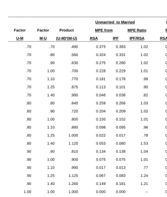
Table 1: Mean proportional errors of RSA and IPF rate estimates in the context of a two-state (married/unmarried) life table model based on the experience of Swedish females born 1930-34
Unmarried to Married Married to Unmarried
Factor Factor Product MPE from MPE Ratio MPE from MPE Ratio
U-M M-U (U-M)*(M-U) RSA IPF IPF/RSA RSA IPF IPF/RSA
.70 .70 .490 0.375 0.383 1.02 0.181 0.188 1.04
.70 .80 .560 0.324 0.331 1.02 0.146 0.154 1.06
.70 .90 .630 0.275 0.280 1.02 0.113 0.123 1.09
.70 1.00 .700 0.228 0.229 1.01 0.082 0.093 1.14
.70 1.10 .770 0.181 0.178 .99 0.067 0.080 1.19
.70 1.25 .875 0.113 0.101 .90 0.048 0.063 1.31
.70 1.40 .980 0.046 0.038 .82 0.036 0.053 1.48
.80 .80 .640 0.259 0.266 1.03 0.122 0.129 1.05
.80 .90 .720 0.204 0.209 1.02 0.087 0.095 1.09
.80 1.00 .800 0.150 0.152 1.01 0.054 0.063 1.18
.80 1.10 .880 0.098 0.095 .96 0.037 0.048 1.29
.80 1.25 1.000 0.022 0.017 .78 0.023 0.035 1.54
.80 1.40 1.120 0.053 0.080 1.53 0.065 0.049 .76
.90 .90 .810 0.134 0.138 1.04 0.062 0.066 1.07
.90 1.00 .900 0.075 0.075 1.01 0.026 0.032 1.22
.90 1.10 .990 0.017 0.013 .77 0.011 0.018 1.64
.90 1.25 1.125 0.067 0.083 1.24 0.055 0.045 .83
.90 1.40 1.260 0.149 0.181 1.21 0.100 0.088 .88
1.00 1.00 1.000 0.000 0.000 -- 0.000 0.000
--1.00 1.10 1.100 0.063 0.069 1.10 0.035 0.034 .97
1.00 1.25 1.250 0.155 0.174 1.12 0.086 0.083 .97
1.00 1.40 1.400 0.245 0.281 1.15 0.133 0.128 .96
1.10 1.10 1.210 0.142 0.149 1.05 0.063 0.071 1.12
1.10 1.25 1.375 0.241 0.263 1.09 0.116 0.122 1.06
1.10 1.40 1.540 0.338 0.379 1.12 0.166 0.171 1.03
1.25 1.25 1.563 0.368 0.395 1.07 0.160 0.187 1.17
1.25 1.40 1.750 0.476 0.525 1.10 0.213 0.241 1.13
Table 1 shows the overall errors found when every value of FUM was combined with every equal or higher value of FMU. The measure of accuracy used is the Mean Proportional Error (MPE) where the proportional error is
PE = ( Actual - Estimated) / Actual (5)
Since the principal marriage ages are approximately 15-39, the MPE values shown in Table 1 reflect the average of the absolute values of the proportional errors for those ages. The IPF/RSA ratio of MPE values is also shown, with a ratio over 1 indicating that the IPF method has a larger error, and a ratio under 1 indicating that the RSA method has a larger error.
Table 1 shows that RSA and IPF yielded fairly similar error levels, though RSA usually did a bit better. When the product of FUM and FMU was close to one, the MPE was small, e.g less than 2% when FUM was .90 and FMU was 1.10. At the extremes, shown in panels A and C of Figure 1, the MPE was from near 40% to over 60%. As is true for indirect standardization, the results are thus standard dependent. Standards that yield offsetting changes in the rates produce good results for both methods, though all of the standards used led to reasonable marriage patterns over age. It is not surprising that the RSA estimates go increasingly off as the underlying state attraction assumption increasingly departs from the actual circumstances. What is surprising is that the IPF estimates go off in very much the same way, even though its underlying assumptions are quite different.
4.1.2. Models with four living states
Table 2: Mean Proportional Errors of RSA and IPF Rate Estimates in the Context of a Four State Marital Status Life Table Based on the Experience of United States Females in the Year 1995.
All Marriage Rates
Divorce
Rate Single to Married Married to Divorced Divorced to Married
Factor Factor Product MPE from
MPE
Ratio MPE from
MPE
Ratio MPE from
MPE Ratio
U-M M-V (U-M)*(M-V) RSA IPF IPF/RSA RSA IPF IPF/RSA RSA IPF IPF/RSA
.70 .70 .490 0.007 0.007 1.01 0.181 0.181 1.00 0.397 0.396 1.00
.70 .80 .560 0.007 0.007 1.00 0.152 0.153 1.00 0.336 0.336 1.00
.70 .90 .630 0.006 0.006 .99 0.125 0.126 1.00 0.278 0.278 1.00
.70 1.00 .700 0.006 0.006 .97 0.099 0.100 1.01 0.221 0.223 1.01
.70 1.10 .770 0.005 0.005 .95 0.074 0.076 1.02 0.167 0.170 1.02
.70 1.25 .875 0.005 0.005 .92 0.039 0.041 1.05 0.089 0.094 1.05
.70 1.40 .980 0.005 0.004 .88 0.005 0.009 1.66 0.015 0.021 1.46
.80 .80 .640 0.004 0.004 1.01 0.122 0.121 1.00 0.269 0.268 1.00
.80 .90 .720 0.004 0.004 .99 0.092 0.093 1.00 0.206 0.206 1.00
.80 1.00 .800 0.004 0.004 .97 0.064 0.065 1.01 0.144 0.146 1.01
.80 1.10 .880 0.003 0.003 .94 0.038 0.039 1.04 0.085 0.088 1.03
.80 1.25 1.000 0.003 0.002 .88 0.001 0.003 5.30 0.001 0.006 11.16
.80 1.40 1.120 0.002 0.002 .86 0.037 0.033 .91 0.081 0.073 .91
.90 .90 .810 0.002 0.002 1.02 0.061 0.061 1.00 0.137 0.136 1.00
.90 1.00 .900 0.002 0.002 .97 0.031 0.032 1.02 0.071 0.072 1.01
.90 1.10 .990 0.001 0.001 .90 0.003 0.004 1.47 0.007 0.010 1.35
.90 1.25 1.125 0.001 0.001 .84 0.038 0.035 .94 0.084 0.079 .94
.90 1.40 1.260 0.001 0.001 .96 0.076 0.073 .95 0.172 0.163 .95
1.00 1.00 1.000 0.000 0.000 -- 0.000 0.000 -- 0.000 0.000
--1.00 1.10 1.100 0.000 0.000 1.31 0.030 0.029 .97 0.068 0.066 .97
1.00 1.25 1.250 0.001 0.001 1.35 0.073 0.071 .97 0.165 0.160 .97
1.00 1.40 1.400 0.001 0.002 1.39 0.114 0.110 .97 0.259 0.250 .97
1.10 1.10 1.210 0.002 0.002 1.02 0.062 0.062 1.00 0.140 0.139 .99
1.10 1.25 1.375 0.002 0.002 1.09 0.107 0.105 .98 0.244 0.239 .98
1.10 1.40 1.540 0.003 0.003 1.14 0.150 0.146 .97 0.342 0.334 .97
1.25 1.25 1.563 0.004 0.004 1.02 0.156 0.155 .99 0.356 0.353 .99
1.25 1.40 1.750 0.004 0.005 1.06 0.202 0.198 .98 0.463 0.455 .98
Figure 2 shows the three rates of interest when the factors FUM and FMV are (.7, .7), (.7, 1.4), and (1.4, 1.4). Once again, when the product of the factors is close to one (as in panel B), both methods closely reproduce the actual rates. Estimates of msm are consistently good (under 1%) for both methods, because the Never Married state has no entrants, and thus there are no complications from a transfer rate from Presently Married to Never Married. Estimates of mmv and mvm are increasingly in error as the product of the factors departs from one, though again the two methods generate similar estimates and produce a reasonable pattern over age. When the factors are both below one or both above one (Panels A and C of Figure 2), the mmv estimates are between the standard and actual values, while the mvm estimates are a bit further away from the actual than the standard. Nonetheless, for most factor combinations, the error level is not bad considering the limited input data.
4.2. Evaluations of estimates using actual data for the standard rates
Table 3 shows standard, actual, and RSA and IPF estimates of msm, mmv, and mvm for United States Females, 1995, when the standard is based on observed values for United States Females, 1988. While not far apart in time, the marriage and divorce rates of those two years showed quite different patterns. In 1995, marriage, divorce, and remarriage rates were much lower at young ages but somewhat higher at older ages than they were in 1988. Thus the 1988 standard implies reinforcing, not offsetting, changes in the rates, and affords a demanding test of the RSA approach.
Table 3: Standard (year 1988), actual (year 1995), and estimated rates for U.S. females, using the relative state attraction (RSA) and iterative proportional fitting (IPF) approaches
Single to Married Age Standard Actual RSA IPF
Married to Divorce Standard Actual RSA IPF
Divorced to Married Standard Actual RSA IPF
18 .05701 .02722 .02727 .02728 19 .07184 .05353 .05361 .05368
.10390 .05579 .08814 .08423 .12581 .05593 .09958 .09307
.57823 .03682 .78180 .68688 .54149 .07387 .81975 .69553 20 .10124 .07127 .07135 .07134
21 .12319 .08164 .08173 .08174 22 .13446 .09772 .09780 .09779 23 .12419 .10803 .10805 .10803 24 .10574 .11321 .11322 .11321
.06814 .04766 .07076 .07122 .07107 .04080 .06704 .06582 .06563 .04588 .06991 .07099 .06369 .04347 .06635 .06715 .05863 .04478 .06093 .06155
.50253 .13350 .47543 .48313 .52848 .21473 .58260 .56459 .52997 .17490 .48020 .49464 .53343 .23492 .49972 .50932 .47975 .27526 .45219 .45930 25 .15988 .13640 .13640 .13640
26 .14562 .12927 .12912 .12912 27 .12802 .12540 .12528 .12526 28 .10573 .13309 .13276 .13273 29 .09245 .10172 .10171 .10169
.04692 .04141 .04434 .04406 .04302 .03899 .04285 .04283 .03804 .03804 .04325 .04367 .03567 .03845 .04415 .04486 .03300 .03798 .03762 .03795
.26695 .25661 .28659 .28363 .26159 .22564 .26278 .26268 .23829 .15729 .20423 .20826 .24390 .14234 .18895 .19497 .19695 .17164 .16910 .17165 30 .06657 .08609 .08287 .08279
35 .04198 .05313 .05218 .05170 40 .02084 .03241 .03172 .03076 45 .01186 .01657 .01643 .01556 50 .00732 .01148 .01081 .00942
.02670 .03160 .02788 .02843 .02230 .02582 .02300 .02323 .01900 .02161 .01965 .01989 .01300 .01523 .01257 .01271 .00780 .01041 .00835 .00864
.13770 .15208 .12698 .13100 .09030 .10170 .08599 .08702 .06690 .07196 .06338 .06407 .04640 .05856 .04723 .04746 .03030 .03479 .02720 .02739
Table 4: Selected summary measures from actual 1988, actual 1995, and estimated 1995 female marital status life tables for the United States.
Measure Actual RSA Estimated IPF Estimated
1988 1995 1995 1995
1. PROPORTION EVER MARRYING OF THOSE
SURVIVING TO AGE 15 .879 .887 .886 .884
2. MEAN AGE AT FIRST MARRIAGE 25.1 26.6 26.6 26.6
3. NUMBER OF MARRIAGES PER PERSON
MARRYING 1.51 1.46 1.45 1.46
4. PROPORTION OF MARRIAGES ENDING IN
DIVORCE .432 .425 .415 .419
5. MEAN AGE AT DIVORCE 34.4 37.3 35.5 35.6
6. AVERAGE DURATION OF A MARRIAGE 24.8 25.7 25.8 25.8
7. REMARRIAGES OF WIDOWED
PERSONS/WIDOWHOODS .063 .048 .057 .056
8. REMARRIAGES OF DIVORCED
PERSONS/DIVORCES .723 .687 .695 .695
5. A substantive application
To show how the RSA method can be applied to produce useful results, we estimate rates of interregional migration in the United States for the period 1980-1990. Such rates are not known at present, although rates for the period 1985-90 have been calculated from a retrospective question in the 1990 Census that asked place of residence in 1985. Appendix B describes how 1980 and 1990 Census figures, and life table values for the 1989-91 period, were used to calculate multiregional life tables for the U.S., 1980-90. Four regions were recognized: North-east, Mid-west, South, and West.
Figure 3 compares RSA estimated age-specific female rates into and out of the Mid-west for 1980-90 with analogous rates for 1985-90. There are clear differences between the two, with the entire decade having lower rates of migration into the Mid-west from every other region, and higher rates of migration out of the Mid-west to every other region. That pattern is found in all age groups. Expressing that pattern in terms of RSA assumptions, the Mid-west region exerted more attraction during 1985-90 than it did over the 1980-90 decade.
Table 5: Selected measures from multiregional life tables for United States females, 1980-90 (RSA and IPF estimates) and 1985-90 (actual)
RSA 1980-90 IPF 1980-90 1985-90
A. Number of Moves Per Person
.676 .676 .674
Entrants Exits Net Change
1980-90 1985-90 1980-90 1985-90 1980-90 1985-90
B. Inter-Regional Moves RSA IPF RSA IPF RSA IPF
1. North-east 10,085 10,080 9,681 13,277 13,280 13,841 -3,192 -3,200 -4,160 2. Mid-west 13,967 13,965 15,063 19,029 19,026 17,590 -5,062 -5,061 -2,527 3. South 27,756 27,762 27,465 20,516 20,515 20,579 7,240 7,247 6,886 4. West 15,779 15,782 15,159 14,765 14,768 15,358 1,014 1,014 -199 Total 67,587 67,589 67,368 67,587 67,589 67,368 0 0 0
Note: See Appendix B for calculation details
6. Summary and conclusions
We have developed, evaluated, and applied a new method, based on relative state attraction, that estimates interstate transfer rates from cross-sectional population distributions and an assumed set of standard rates. The RSA method performs as well as the leading alternative, iterative proportional fitting. Unlike IPF, however, RSA has a clear and plausible substantive interpretation and can be used to examine the implications of hypothesized changes in the power of attraction of different states.
A basic characteristic of the RSA method is that the product of the transfer rates between two states (i.e. the product mij mji) is the same in both the assumed standard and the resultant estimates. Hence, relative to the standard chosen, if the rates of transfer from one state (say i) to the other (j) increase, then the rates in the opposite direction are assumed to decrease. The effects of such constraints on the estimates were examined in the context of two-state and four-state models using stylized changes in the standard rates, and in a four state model where estimates were made based on rates observed in a nearby year. The results showed that RSA yields excellent estimates when there are large, compensating changes in interstate rates. When the rates between two states move in the same direction, the estimates are more in error, but nonetheless preserve the age pattern of behavior in the rates and generally yield age-aggregated summary measures close to actual levels.
encouraging, however, because it suggests that one comes to a very similar result regardless of whether the problem is approached from a heuristic, more demographic, perspective or from the viewpoint of statistical estimation.
There are many circumstances where it is useful to estimate behavioral rates when only a standard pattern and two cross-sectional population distributions are known. The procedures developed here show how that can be done in a way that is easy to justify in nontechnical terms, that can be calculated in a straightforward fashion, and that gives results that typically approximate maximum likelihood estimates.
7. Acknowledgements
Notes
1. The present topic has tangential relationships to two other lines of research that are not pursued here. One is estimations from sequential cross sections in the decrement only context (see Schmertmann 2002). The other is estimating fertility and mortality from age distributions via inverse projection (cf. Lee 1985; Oeppen 1993).
2. There are many ways to go from population distribution (l) vectors to person-year (L) vectors. The simplest is the linear assumption, used in the calculations presented here, where
L(t,u) = (u/2)[ l(t) + l(t+u)] (E.1)
An alternative is to estimate the mean duration into the interval at which each type of transfer takes place, i.e. estimate the multistate version of Chiang’s a. That can be done from a number of sources, including adjacent transfer rates (see Schoen 1988: Chapter 4 for a discussion of these and other techniques).
References
Batty, M. and S. Mackie. 1972. The calibration of gravity, entropy and related models of spatial interaction. Environment and Planning 4:205-33.
Bishop, Y.M., S.E. Fienberg, and P.W. Holland. 1975. Discrete Multivariate Analysis:
Theory and Practice. Cambridge MA: MIT Press.
Chilton, R. and R. Poet. 1973. An entropy maximizing approach to the recovery of detailed migration patterns from aggregate census data. Environment and Planning 5:135-46.
Deming, W.E. and F.E. Stephan. 1940. On a least squares adjustment of a sampled frequency table when the expected marginal totals are known. Annals of
Mathematical Statistics 11:427-44.
Furness, K.P. 1965. Time function iteration. Traffic Engineering and Control 7:458-60. Halli,S.S. and K.V. Rao. 1992. Advanced Techniques of Population Analysis. New York:
Plenum.
Kruithof, J. 1937. Calculation of telephone traffic. De Ingenieur 52:E15-E25.
Lee, R.D. 1985. Inverse projection and back projection: A critical appraisal, and comparative results for England, 1539 to 1871. Population Studies 39:233-48. McFarland, D.D. 1975. Models of marriage formation and fertility. Social Forces 54:66-83. Moffitt, R. 1993. Identification and estimation of dynamic models with a time series of
repeated cross-sections. Journal of Econometrics 59:99-123.
Moffitt, R. and M. Rendall. 1995. Cohort trends in the lifetime distribution of female family headship in the United States, 1968-1985. Demography 32:407-24.
Nair, P.S. 1985. Estimation of period-specific gross migration flows from limited data: Bi-proportional adjustment approach. Demography 22:133-42.
Oeppen, J. 1993. Back projection and inverse projection: Members of a wider class of constrained projection models. Population Studies 47:245-67.
Philipov, D. 1978. Migration and settlement in Bulgaria. Environment and Planning A 10:593-617.
Ruggles, S. and M. Sobek et al. 1997. Integrated Public Use Microdata Series: Version
2.0. Minneapolis: Historical Census Projects, Univ. of Minnesota.
(www.ipums.org).
Schoen, R. 1988. Modeling Multigroup Populations. New York: Plenum.
Schoen, R. and N. Standish. 2001. The retrenchment of marriage: Results from marital status life tables for the United States, 1995. Population and Development Review 27:553-63.
Schmertmann, C.P. 2002. A simple method for estimating age-specific rates from sequential cross sections. Demography 39:287-310.
U.S. National Center for Health Statistics. 1997. U.S.Decennial Life Tables for 1989-91, vol 1, no 1. Hyattsville MD.
Willekens, F. 1982. Multidimensional population analysis with incomplete data. Pp 43-111 in K.C. Land and A. Rogers (Eds), Multidimensional Mathematical Demography. New York: Academic Press.
APPENDIX A
Equations for the adjustment factors in a hierarchical two-state model
1. A two-state hierarchical model can be described by the equations
l1(t+u) = l1(t) - L1(t,u) [ m12(t,u) k2(t,u) / k1(t,u) + m(t,u) / k1(t,u) ]
l2(t+u) = l2(t) - L2(t,u) m(t,u) / k2(t,u) + L1(t,u) m12(t,u) k2(t,u) /k1(t,u) (A.1)
ZKHUH LQGLFDWHVWKHGHDGVWDWH7KHUHDUHWUDQVIHUVIURPVWDWHWRVWDWHEXWQRELUWKV and no transfers from state 2 to state 1. The solutions for k1(t,u) and k2(t,u) are
k2(t,u) = [ l1(t) k1(t,u) - l1(t+u) k1(t,u) - L1(t,u) m(t,u) ] / [L1(t,u) m12(t,u)] (A.2)
where k1(t,u) is the positive root of the quadratic equation
0 = [k1(t,u)]2 { [l1(t) - l1(t+u)]2 + [l1(t) - l1(t+u)] [l2(t) - l2(t+u)] }
+ k1(t,u)L1(t,u) { m(t,u)[2 l1(t+u)-2 l1(t)+l2(t+u)-l2(t)] - L2(t,u) m(t,u) m12(t,u) }
+ [ L1(t,u) m(t,u) ]2 (A.3)
2. A two-state non-hierarchical model with no fertility or mortality can be described by the equations
l1(t+u) = l1(t) - Z L1(t,u) m12(t,u) + L2 (t,u) m21(t,u) / Z
l2(t+u) = l2(t) - L2(t,u) m21(t,u) / Z + Z L1(t,u) m12(t,u) (A.4)
where Z = k2(t,u) / k1(t,u). Using the first equation in (A.4) and solving the quadratic yields
Z = [1/(2 L1(t,u) m12(t,u))] [{l1(t) - l1(t+u)} ± [{l1(t) - l1(t+u)}2
+ 4 L1(t,u) m12(t,u) L2(t,u) m21(t,u)]½] (A.5)
APPENDIX B
Calculating multiregional life tables for the United States, 1980-90
The population data for the calculations were obtained from the Integrated Public Use Microdata Series (IPUMS, available at www.ipums.org/usa/doc.html; see Ruggles and Sobek et al 1997). From the 1980 and 1990 census public use microdata 5% samples, information was extracted on the age, sex, state of residence, state of birth (only U.S. born persons were included), person sampling weight, and (for 1990) state of residence in 1985. States were aggregated into 4 regions: North-east (Connecticut, Maine, Massachusetts, New Hampshire, New Jersey, New York, Pennsylvania, Rhode Island, and Vermont), Mid-west (Illinois, Indiana, Iowa, Kansas, Michigan, Minnesota, Missouri, Nebraska, North Dakota, Ohio, South Dakota, and Wisconsin), West (Alaska, Arizona, California, Colorado, Hawaii, Idaho, Montana, Nevada, New Mexico, Oregon, Utah, Washington, Wyoming), and South (the remaining states and the District of Columbia). Throughout, mortality in all regions was assumed to follow that of the U.S Life Tables for 1989-91 (U.S. National Center for Health Statistics 1997).
To prepare the multiregional life tables for 1985-90, the male and female populations were each put in 5-year age groups for ages 0-4 through 80-84 years, with ages 85 and over combined. The calculation procedure followed was essentially that described in Schoen (1988:76-79). For ages 5-9 through 80-84, retrospective proportions Rij were calculated as the ratio of (a) the number in state i in 1985 who were in state j in 1990 to (b) the sum over all regions j of those who were in state i in 1985 and in state j in 1990. Survivorship proportions Sij were calculated from the Rij by back surviving the total 1990 population to 1985, using the 1989-91 U.S. female life table. Migration at ages over 85 was assumed to be the same as at ages 80-84. State of birth was used as the previous state for persons aged 0-4 in 1990. Elements of the Markov transition probability matrices ( ) were then found as the arithmetic mean of the Sij for that and the preceding age interval. The (i,j) element of is the probability that a person in state j at the beginning of an interval is in state i at the end of the interval. The matrix of interstate transfer rates was then obtained by the linear relationship M=(2/5)[I+ ]-1[I- ], where I represents the identity matrix. The life table was calculated using a program very similar to Program IDLT in Schoen (1988:Appendix D), but with linear survivorship. The initial number of persons in each state was allocated in proportion to the reported state of birth of persons under 5 in the 1990 Census.