Volume 21 - Article 28 | Pages 843–878

(1)

in the population sciences published by the Max Planck Institute for Demographic Research Konrad-Zuse Str. 1, D-18057 Rostock · GERMANY www.demographic-research.org

DEMOGRAPHIC RESEARCH

VOLUME 21, ARTICLE 28 PAGES 843-878

PUBLISHED 08 DECEMBER 2009

http://www.demographic-research.org/Volumes/Vol21/28/ DOI: 10.4054/DemRes.2009.21.28

Descriptive Finding

Assortative matching among same-sex

and different-sex couples in the United States,

1990-2000

Christine R. Schwartz

Nikki L. Graf

This open-access work is published under the terms of the Creative Commons Attribution NonCommercial License 2.0 Germany, which permits use, reproduction & distribution in any medium for non-commercial purposes, provided the original author(s) and source are given credit.

(2)

1 Introduction 844

2 Previous research 846

3 Data and methods 847

3.1 The sample 847

3.2 Identifying same-sex couples 848

3.3 Measures 850

3.4 Statistical models 850

4 Results 853

4.1 Descriptive statistics 853

4.2 Model fit 854

4.3 Assortative matching by couple type for couples aged 20 to 34 857 4.4 Assortative matching by couple type for couples aged 20 to 49 864

5 Discussion 869

6 Acknowledgments 871

References 872

(3)

Assortative matching among same-sex and

different-sex couples in the United States, 1990-2000

Christine R. Schwartz1

Nikki L. Graf2

Abstract

Same-sex couples are less likely to be homogamous than different-sex couples on a variety of characteristics including race/ethnicity, age, and education. This study confirms results from previous studies which used 1990 U.S. census data and extends previous analyses to examine changes from 1990 to 2000. We find that same-sex male cohabitors are generally the least likely to resemble one another, followed by same-sex female cohabitors, different-sex cohabitors, and different-sex married couples. Despite estimated growth in the numbers of same-sex couples in the population and the increasing acceptance of same-sex unions, we find little evidence of diminishing differences in the resemblance of same- and different-sex couples between 1990 and 2000, with the possible exception of educational homogamy.

1_{Department of Sociology, University of Wisconsin-Madison, 1180 Observatory Drive, Madison, WI 53706.}

(4)

1. Introduction

Family change over the past half century has been marked by an increasing diversity of family forms and an increasing acceptance of nontraditional relationships (Cherlin 2004; Thornton and Young-DeMarco 2001). Cohabitation, nonmarital childbearing, interracial and interreligious relationships, and same-sex unions have all become more common (Casper and Bianchi 2002; Gates 2007; Rosenfeld 2008). Scholars have often compared emerging and nontraditional relationships to more traditional ones to better understand their characteristics. For example, a large body of research compares the characteristics of cohabitors and married couples in an effort to determine what cohabitation “is” and where it fits into the American family system (for reviews see Seltzer 2000, 2004; Smock 2000). This paper takes a similar approach to the study of same-sex coresidential unions. Despite much attention to gay and lesbian couples in the press and policy realms, there is still relatively little systematic research on similarities and differences between same- and different-sex couples. In this paper, we compare the resemblance of partners in same- and different-sex coresidential couples, or who is partnered with whom. Gay men and lesbians may choose different types of partners than heterosexuals because of differences in the characteristics of their partner markets and/or because of differences in their preferences for partners.

(5)

have more opportunities to match outside their own race/ethnic or educational group. Each of these hypotheses suggests that same-sex couples will be more likely than different sex-couples to form relationships across social boundaries. Previous research is consistent with this claim, showing that same-sex couples tend to resemble one another less than different-sex couples on a variety of characteristics (Andersson et al. 2006; Jepsen and Jepsen 2002; Kurdek and Schmitt 1987; Rosenfeld 2007; Rosenfeld and Kim 2005).

This paper examines couple resemblance among four types of coresidential couples: same-sex male unmarried couples, same-sex female unmarried couples, different-sex unmarried couples, and different-sex married couples. Using data from the 5% samples of the U.S. decennial census, we confirm results from previous studies showing less couple resemblance among same-sex couples than among different-sex couples and extend previous studies by examining changes in matching patterns from 1990 to 2000. Previous research has either examined differences in assortative matching in a single time period or cohort (Andersson et al. 2006; Jepsen and Jepsen 2002; Kurdek 2003; Kurdek and Schmitt 1987), or has focused on matching on a single characteristic (Rosenfeld and Kim 2005). We provide a more detailed account of differences in assortative matching by couple type across three dimensions— race/ethnicity, age, and education—and describe how these patterns changed between 1990 and 2000. By most estimates, the numbers of same-sex couples in the population increased over this period as same-sex and other nontraditional relationships have become more accepted (Gates 2006, 2007; Loftus 2001; Rosenfeld 2007; Thornton and Young-DeMarco 2001). Thus, we might expect differences between same- and different-sex relationships to have declined as same-sex couples have become a less select group and as same-sex relationships have become less nonnormative (Rosenfeld and Kim 2005).

(6)

2. Previous research

Previous research has found that same-sex couples tend to be less alike, or are less likely to be homogamous, than different-sex couples (Andersson et al. 2006; Jepsen and Jepsen 2002; Kurdek and Schmitt 1987; Rosenfeld and Kim 2005). Furthermore, matching patterns differ by the sex composition of the couple—same-sex male couples tend to resemble each other less than same-sex female couples (Andersson et al. 2006; Jepsen and Jepsen 2002). Recently, Jepsen and Jepsen (2002) provided the first multivariate analysis of matching patterns among same- and different-sex couples using nationally representative data. Using 1990 U.S. census data, Jepsen and Jepsen found evidence of positive assortative matching for both same- and different-sex couples on non-labor-market traits such as age, education, race, investment income, as well as for labor-market traits, including earnings and hours worked, although to a lesser extent. For most non-labor-market traits (e.g., age, race), members of different-sex married couples were the most similar, followed by members of different-sex cohabiting couples, who were in turn more similar than members of same-sex couples. By contrast, for labor-market traits (e.g., hourly earnings), members of married couples were the least similar of all couple types, highlighting the division of household and market labor between husbands and wives. Other studies have largely relied on relatively small, nonrepresentative samples, but show similar results (Kurdek 2003; Kurdek and Schmitt 1987).

(7)

3. Data and methods

3.1 The sample

We use the 5% samples of the 1990 and 2000 U.S. censuses from the Integrated Public Use Microdata Series (IPUMS) to examine assortative matching patterns among same- and different-sex couples (Ruggles et al. 2004). Beginning in 1990, the census included a category on the household roster for “unmarried partner.” We use this item in conjunction with marital status and sex to identify four types of coresidential couples: same-sex male cohabiting couples, same-sex female cohabiting couples, different-sex cohabiting couples, and different-sex married couples. We exclude same-sex couples who reported being married for reasons discussed below.

In defining our sample for 1990 and 2000, we exclude couples living in group quarters, as well as those for whom age, sex, or relationship to the householder was imputed (following Black et al. 2000:144-46) (N = 4,972,695). In addition, we drop households in which the household head reported having more than one spouse or partner and households in which the household head was excluded due to sample restrictions (N = 4,713,634).3_{The 1990 and 2000 censuses do not contain information} with which to directly identify when couples began living together or when they were first married. Therefore, our data represent a cross-section of all coresiding couples in the population at a given time, or “prevailing unions.” This means that the patterns of couple resemblance we observe are not only the result of assortative matching but are also affected by selective union dissolution and changes in partners’ characteristics after union formation. Although this is a limitation of the data, if same-sex couples (for instance) are more tolerant of differences in their partners, then we would expect same-sex couples to both be more likely to choose and remain with dissimilar partners than different-sex couples. To partially counteract the effects of selective union dissolution and to minimize cohort overlap between 1990 and 2000, however, we restrict our sample to couples in which both partners were between the ages of 20 and 34 at the

3_{We define all couple types according to their relationship to the household head; therefore, couples in which}

(8)

time of the census (N = 1,111,998 couples).4_{Because our sample of 20 to 34 year old} same-sex couples is relatively small despite the very large size of our total sample, we also estimate our models using a wider age interval as a robustness check, including all couples in which both partners are between the ages of 20 and 49 (N = 3,172,977 couples).

3.2 Identifying same-sex couples

A comprehensive review of data on same-sex couples using the 1990 census, the General Social Survey (GSS), and the National Health and Social Life Survey (NHSLS) concluded that the 1990 census, although not without its problems, is a credible source of data for empirical studies of the gay and lesbian population (Black et al. 2000). However, a change in the Census Bureau’s procedure for handling same-sex couples complicates comparisons of assortative matching by couple type between 1990 and 2000. In 1990, records in which the household head identified someone of the same sex as a “husband/wife” were most often edited so that the sex of the “husband/wife” was changed (Gates and Sell 2007). While this procedure exacerbates the undercount of same-sex couples in the U.S., analyses of these data suggest that same-sex couples in the 1990 census are very likely to be “true” same-sex couples (Black et al. 2000, 2007). By contrast, analyses of the 2000 census suggest that data on same-sex couples are highly contaminated by different-sex married couples in which the wrong sex was marked for one of the spouses (Black et al. 2007). This problem occurred because same-sex “spouses” were changed to “unmarried partners” to comply with the 1996 Defense of Marriage Act (H.R. 3396) in the 2000 census data. Black et al. (2007) estimate that over 40% of same-sex “unmarried partner” couples in the 2000 census are actually different-sex married couples in which sex was miscoded.

To obtain comparable samples of same-sex couples in 1990 and 2000, we follow Black et al.’s (2007) recommendation of excluding same-sex couples with edited marital status values. Rosenfeld and Kim (2005) also used this procedure and found that it improved the comparability of the samples. Excluding couples in which either partner’s marital status was edited reduces the overall sample size of couples aged 20 to 34 by a very small percentage (0.58% in 1990 and 1.37% in 2000), but reduces the sample of same-sex male couples by 35% and the sample of same-sex female couples

4_{We select our sample based on the ages of both partners because of the arbitrariness of selecting on one or}

the other partner’s ages in same-sex relationships. The results do not differ substantially from those presented here when we relax this restriction and use a sample of women aged 20 to 34 with different-sex

(9)

by 42% (total N for couples aged 20 to 34 = 1,101,499; N for same-sex male couples = 2,296; Nfor same-sex female couples = 2,329).5_{Doing so also means that our sample} of same-sex couples is representative of same-sex couples in the U.S. who self-identified as “unmarried partners” rather than the population of all same-sex coresidential couples.

Same-sex couples who self-identify as “unmarried partners” may have quite different patterns of assortative matching than those who identify as married. Previous research on different-sex couples has shown that as relationships move from cohabitation to marriage they are less likely to be interracial (Joyner and Kao 2005). If this pattern holds for same-sex couples, then those who self-identify as married may be more likely to be homogamous than “unmarried partner” couples. On the other hand, Carpenter and Gates (2008) find that same-sex couples who officially register their partnerships with their local or state governments are more likely to be highly educated than those who are not registered. To the extent that highly educated individuals are more likely to form relationships that cross social boundaries (Rosenfeld 2007), same-sex couples who self-identify as married may be less likely to be homogamous than “unmarried partner” couples.

If same-sex couples who report being married are systematically more or less likely to be homogamous than couples who self-identify as “unmarried partners,” then excluding same-sex couples who report being married may present a problem for our analysis if the proportion of same-sex coresidential couples who self-identify as married has grown. If this is the case, then changes (or the lack thereof) in assortative matching among same-sex couples may be due to differential selection of same-sex couples out of the “unmarried partner” category and into the “married” category. For example, same-sex couples overall may have become more likely to be homogamous between 1990 and 2000, but we may not observe this trend if homogamous couples were more likely to report being married in 2000. Thus, our findings on change over time should be interpreted with caution.

Despite our focus on unmarried same-sex coresidential couples rather than all same-sex coresidential couples, data from both 1990 and 2000 provide important information about differences in partner resemblance by couple type. In particular, if same-sex couples in more serious relationships are increasingly likely to identify as married, we might expect those who identify as “unmarried partners” to increasingly resemble different-sex cohabitors. To the extent that the resemblance of same-sex cohabiting couples remains lower than that of different-sex cohabiting couples, gay men’s and lesbians’ constrained partner markets and/or their greater tolerance of

(10)

differences in their mates may provide an explanation. It should also be noted that it is not only who is a same-sex “unmarried partner” that has changed between 1990 and 2000. We study “moving targets” when we study each of these types of relationships (Seltzer 2000). The characteristics of married, cohabiting, and same-sex cohabiting relationships have all changed over time, which is an important motivation for studying family change. For example, some predict that as cohabitation becomes the norm in societies, differences in the attitudes and behaviors of cohabitors and married couples will decline (Hamplova 2009). Similarly, as same-sex relationships become more common, differences between same-sex cohabitors and different-sex cohabitors may also decline.

3.3 Measures

We examine assortative matching by couple type on race/ethnicity, education, and age. Our race/ethnic classification is based on individuals’ self-reports on the census questionnaire. Our classification distinguishes among Hispanic whites, non-Hispanic African Americans, non-Hispanics, and those in all other race/ethnic groups. Hispanics are those who identify as persons of Hispanic/Spanish/Latino origin. In the 2000 census, the Census Bureau changed its race classification, allowing respondents to choose one or more race categories whereas previously, respondents could indicate belonging only to a single race. In an analysis of the effects of this change on race/ethnic intermarriage, Qian and Lichter (2007) find that changes in intermarriage are more comparable between 1990 and 2000 if biracial whites are classified as white. Thus, following Qian and Lichter (2007), we classify biracial whites as white in 2000. We use a four-category classification of individuals’ education based on the highest level attained: less than high school, high school (includes those with a GED), some college (includes those with associate degrees), and college or above.

3.4 Statistical models

(11)

availability or preferences over and above differences in demographic characteristics, differences in matching by couple type should still be evident after controlling for these characteristics.

In this paper, we use multinomial logit models which produce coefficients and standard errors that are equivalent to those of log-linear models but are more parsimonious (DiPrete 1990; Logan 1983; see Appendix A for a discussion of the formal relationship between the multinomial logit models used here and log-linear models). To incorporate our covariates and examine differences in assortative matching by couple type, we estimate a multinomial logit model that predicts couple type as a function of couples’ characteristics. Our baseline model assumes that couples’ background characteristics differ but that the likelihood of matching assortatively does not vary by couple type. Formally, our baseline model is:

1 ( )

log 2,..., 4

( ) j

j j j

π

α

π = + ′ =

x

β x

x (1)

where πj( )x =⎣⎡P Y

(

= jx

)

⎤⎦, Y denotes the couple type (j=1,…,4; different-sex

married, different-sex cohabiting, same-sex female, same-sex male) and x is a vector of the characteristics of both partners (race/ethnicity, education, and age) interacted with census year, which allows the association between demographic characteristics and couple type to vary over time. The x variables are defined as shown in Table 1, with the exception of age, which is classified into three categories: 20-24, 25-29, and 30-34. We do this to preserve the integrity of the relationship between log-linear and multinomial logit models. We add terms to capture differences in assortative matching by couple type as follows:

1 ( , )

log 2,..., 4

( , ) j

j j j j

π

α

π = + ′ + ′ =

x z

β x δ z

x z (2)

where the z variables are indicators of assortative matching, the δs are differences in the log odds of assortative matching between couples of type j and different-sex married couples, and all other terms are as defined above. Jepsen and Jepsen (2002) employ a similar strategy but instead of a multinomial logit model comparing all four couple types, they present binary logit models to compare assortative matching between same- and different-sex couples.

(12)

type of relationship. Rather, we view our multinomial logit model as a convenient way of summarizing differences in assortative matching by couple type while controlling for differences in couples’ characteristics.

Table 1: Characteristics of individuals aged 20 to 34 in coresidential unions by couple type, 1990-2000

Same-Sex Cohabiting

Male

Same-Sex Cohabiting Female

Different-Sex Cohabiting

Different-Sex Married

1990 2000 1990 2000 1990 2000 1990 2000

Age

Mean 28.02 28.04 28.06 27.42 26.64 26.48 28.42 28.55

SD 3.67 4.06 3.61 3.93 3.87 3.84 3.59 3.57

Race/Ethnicity (%)

White 83.9 75.5 84.7 74.7 75.2 69.5 80.9 72.1

Black 5.2 7.2 6.0 11.0 11.9 12.1 6.4 6.6

Hispanic 8.6 13.7 7.1 11.1 9.9 14.3 9.3 16.0

Other 2.4 3.6 2.3 3.2 3.0 4.1 3.3 5.3

Educational Attainment

Less than High School 4.6 6.9 4.9 6.5 15.7 12.6 10.7 10.6

High School 17.4 22.7 15.3 21.0 37.5 33.4 35.9 28.7

Some College 37.9 35.8 36.8 37.6 31.5 34.1 32.0 32.5 College and Above 40.0 34.7 43.0 34.8 15.3 20.0 21.4 28.2

Partner Resemblance

Correlation between

Partners' Ages 0.369 0.477 0.466 0.490 0.453 0.511 0.620 0.627 Race/Ethnic

Endogamy (%) 83.4 79.5 87.0 82.8 88.6 85.8 93.5 91.4 Educational

Homogamy (%) 51.2 52.9 55.1 55.4 50.4 51.8 54.1 56.7

N 2,036 2,556 1,668 2,990 117,056 161,036 1,073,330 842,326

(13)

4. Results

4.1 Descriptive statistics

Table 1 shows descriptive statistics for the variables included in our analysis by couple type and year.6_{On average, individuals in same-sex cohabiting unions are somewhat} older than those in different-sex cohabiting unions and somewhat younger than those in different-sex marriages. The race/ethnic distributions for those in same-sex male and female unions are similar, although those in same-sex female unions are somewhat more likely to be African American. What stands out most is that individuals in same-sex unions are more likely to be white than those in different-same-sex unions. Individuals in different-sex cohabiting unions are the least likely of any couple type to be white. Those in same-sex unions also tend to have higher levels of education than other couple types, a finding that is consistent with previous research (e.g., Black et al. 2000; Phua and Kaufman 1999). In 1990, about 40% of individuals in same-sex male and female cohabiting unions had completed college compared with only 15% of those in different-sex cohabiting unions and 21% of those in different-different-sex marital unions. By 2000, these differences had diminished. In 2000, less than 35% of those in same-sex male and female cohabiting unions had completed college compared with 20% of those in different-sex cohabiting unions and 28% of those in different-sex marital unions. Part of this trend may be due to an increased willingness of same-sex couples with low levels of education to identify themselves as such on government surveys and part may be due to growing numbers of these couples in the population. In either case, these findings suggest that same-sex cohabiting couples in the census have become a less educationally select group.

Table 1 also gives three simple measures of partner resemblance: the correlation between partners’ ages; the percentage of couples who share the same race/ethnicity, or are endogamous (defined using our four-category race/ethnicity classification); and the percentage of couples who share the same educational attainment, or are homogamous (defined using our four-category education classification). Table 1 shows that in 1990 and 2000 the correlation between partners’ ages is lowest for same-sex male couples and highest for different-sex married couples. The correlation between partners’ ages for same-sex female couples is similar to the correlation for different-sex cohabiting couples in both years and falls between same-sex male and different-sex married

6_{Throughout the majority of our analysis the units of observation are couples. To avoid arbitrarily describing}

(14)

couples. The finding that same-sex female couples are more likely to resemble one another on age than same-sex male couples is consistent with previous studies using data from personal advertisements, which show that preferred age differences are larger for gay men than lesbians (Hayes 1995; Over and Philips 1997).

A similar picture emerges from patterns of race/ethnic endogamy. In 1990 and 2000 same-sex male couples were the least likely to be in endogamous unions, followed by same-sex female couples, different-sex cohabitors, and lastly by different-sex married couples. By contrast, patterns of resemblance are somewhat different for educational homogamy. On this measure of matching, same-sex male couples were slightly more likely to be educationally homogamous than different-sex cohabiting couples in both 1990 and 2000. Same-sex female couples were more likely to be homogamous than both same-sex male and different-sex cohabiting couples. In fact, educational homogamy was very similar among same-sex female and different-sex married couples in both years.

Overall, these simple measures of partner resemblance indicate that same-sex male couples are less likely to resemble one another than same-sex female couples. By contrast, whether same-sex female couples or different-sex cohabitors have higher resemblance depends on the characteristic in question. Married couples generally have the highest levels of resemblance, with the exception of education for which same-sex female couples have similar levels of resemblance. These descriptive measures should be interpreted with caution, however, as they may be affected by differences in the characteristics of couples in each of these union types. For example, same-sex female couples may be more likely to be educationally homogamous simply because of their high concentration in the top two education categories. When nearly everyone falls into one or two education categories, it is very likely that individuals will form educationally homogamous unions–this is known as a concentration effect (Simkus 1984). Same-sex couples may also be more likely to be interracial/ethnic because of their high educational attainment as those with high educational attainment are more likely to form interracial unions (Rosenfeld 2007). Thus, in what follows, we control for concentration effects and the possibility that differences in homogamy are the result of differences in the demographic characteristics of those who form these unions by controlling for the marginal distributions of partners’ ages, educational attainments, and race/ethnicities.

4.2 Model fit

(15)

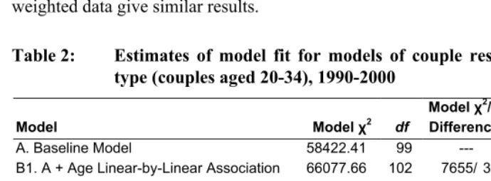
first pooling the 1990 and 2000 census data and then testing whether there is evidence of change in these relationships between years. Table 2 shows estimates of model fit for various models of couple resemblance by couple type. We compare model fit by using the likelihood ratio chi-square test and the Bayesian information criterion (BIC), an index that adjusts the χ2_{statistic for sample size.}7_{More negative BIC statistics indicate} better fitting models. Each model’s fit statistics are compared with those of the model to which new terms are added. We rely mainly on the BIC to choose models because of our very large sample size. The results shown in Table 2 are not weighted as the BIC is a function of the log-likelihood, but Wald tests and BIC statistics calculated using weighted data give similar results.

Table 2: Estimates of model fit for models of couple resemblance by couple type (couples aged 20-34), 1990-2000

Model Model χ2 _df

Model χ2_/_df

Differencea _BIC

BIC Differencea

A. Baseline Model 58422.41 99 --- -57045 ---

B1. A + Age Linear-by-Linear Association 66077.66 102 7655/ 3 -64659 -7614 B2. A + |Age Difference| 66084.04 102 7662/ 3 -64665 -7620 C1. B2 + Race/Ethnic Endogamy 69578.60 105 3495/ 3 -68118 -3453 C2. B2 + Race/Ethnic Variable Endogamy 69630.59 114 3547/ 12 -68045 -3380 D1. C1 + Educational Homogamy 69951.05 108 372/ 3 -68449 -331 D2. C1 + |Education Difference| 69928.15 108 350/ 3 -68426 -308 D3. C1 + Education Crossings Parameters 70345.32 114 767/ 9 -68759 -642 E1. D3 + Association Measures x Year 70507.48 129 162/ 15 -68713 46

Notes: a_"Model_χ2_/_df_{Difference" and "BIC Difference" refer to the difference between the model in a given row and the model to}

which terms are being added, e.g., these columns compare Model B2 to Model A and Model D3 to Model C1. All of the Model χ2

differences are statistically significant at p < 0.01. Results are not weighted. N = 1,101,499.

Model A is the baseline model shown in equation (1) above. It assumes that there are no differences in assortative matching by couple type but accounts for differences in the demographic characteristics of couples and variation in these characteristics by year. In the next series of models, we test various measures of time-invariant differences in assortative matching by couple type.8_{Models B1 and B2 test two specifications of}

7_{The BIC statistic is –}_χ2₊_df_(log_n_{) where}_χ2_{is the likelihood ratio test statistic for testing the null model} against the model of interest (model χ2_),_df_{is the model degrees of freedom (number of independent variables} in the model), and n is the number of observations in the sample (Raftery 1995).

8_{Sensitivity tests showed that the order in which these terms are added to the models does not affect the}

(16)

differences in assortative matching on age. Model B1 represents differences in assortative matching on age using a linear-by-linear association term, which is conceptually similar to a correlation coefficient (Agresti 2002:369-370). Model B2 uses the absolute value of the difference between partners’ ages, a measure similar to that used by Jepsen and Jepsen (2002).9_{A comparison of the}_χ2_{and BIC statistics and their} improvement over Model A indicates that differences in assortative matching by couple type are better described by the absolute value of the difference in partners’ ages rather than a linear-by-linear association, albeit by a very small margin.

Models C1 and C2 add various specifications of differences in assortative matching by couple type on race/ethnicity to Model B2. Model C1 represents these differences with a single dichotomous variable that equals 1 when couples match within race/ethnic groups (as defined in Table 1), or are endogamous, and 0 when couples match across race/ethnic groups. This model assumes that couple types differ in their tendency to pair across race/ethnic groups but that these differences do not vary by the race/ethnic group in question. According to this model, for example, the odds of endogamy may differ for African Americans and Hispanics, but these odds are uniformly higher or lower by couple type. Model C2 allows differences in the odds of race/ethnic endogamy to vary both by race/ethnic group and by couple type. The more negative BIC statistic for Model C1 indicates that it is adequate to describe differences in assortative matching in terms of a single parameter indicating the varying tendencies of the four types of couples to match endogamously on race/ethnicity.

Models D1 through D3 add various specifications of matching on education to Model C1. Model D1 adds a term for educational homogamy, that is, whether or not both partners are in the same education category (as defined in Table 1). Model D2 uses the absolute difference between partners’ years of schooling completed, which is again a measure similar to that used by Jepsen and Jepsen (2002). Finally, Model D3 adds terms for whether or not a couple crosses an educational boundary. This model represents the association between partners’ educational attainments as a series of barriers to partnership between educational groups (see Powers and Xie 2000:117-119 for details). Specifically, assortative matching on education is parameterized in terms of the relative odds of crossing one of three adjacent educational barriers corresponding to the four educational categories shown in Table 1. The exponentiated parameter estimates from the crossings models may be multiplied to calculate the odds of crossing

9_{The linear-by-linear association model (Model B1) estimates}_δ_u

ivj where uiis the male partner’s age in

different-sex relationships and the head of household’s age in same-sex relationships, vj is the female

partner’s age in different-sex relationships and the “unmarried partner” in same-sex relationships, and δis the parameter to be estimated. Scalar values of 22, 27, and 32 years, respectively, are assumed for ui and vj, that

(17)

more distant barriers. By the BIC, the crossings model (Model D3) provides the best fit to the data. Finally, Model E1 allows each of the preferred measures of assortative matching on age, race/ethnicity, and education to vary over time. Although this model is not preferred to Model D3 by the BIC, we present results from Model E1 below since this will allow us to examine how the matching parameters vary over time.10

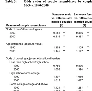
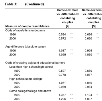
4.3 Assortative matching by couple type for couples aged 20 to 34

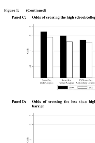
Table 3 shows differences in couple resemblance by couple type estimated from Model E1 (results are weighted using household-level probability weights). For ease of discussion, we refer to “differences” in assortative matching by couple type, but the measures shown in Table 3 are odds ratios. For race/ethnicity, they are the ratios of the odds of endogamy for a given couple type relative to a comparison group. Similarly, for education, they are the ratios of the odds of crossing an educational barrier for a given couple type relative to a comparison group. The age difference parameters are also odds ratios; their interpretation is discussed below. We present measures of couple resemblance for all possible combinations of couples: columns [1] through [3] show the odds of couple resemblance relative to different-sex married couples, columns [4] and [5] show the odds relative to different-sex cohabiting couples, and column [6] shows the odds relative to same-sex female couples. Figure 1 illustrates our estimates of assortative matching on race/ethnicity, age, and education. One drawback of using multinomial logit models is that only the odds of matching relative to the odds for a comparison group are identified; the absolute levels (odds rather than odds ratios) of matching by couple type are not identified. Figure 1 is produced by estimating the odds of assortative matching for different-sex married couples using log-linear models and the levels of assortative matching for the other relationship types using the odds ratios shown in Table 3 (see Appendix A for details).

10_{Model E1 estimates assortative matching on a given characteristic (e.g., race/ethnicity) by couple type net}

(18)

Table 3: Odds ratios of couple resemblance by couple type (couples aged 20-34), 1990-2000

Measure of couple resemblance

Same-sex male vs. different-sex married couples

[1]

Same-sex female vs. different-sex married couples

[2]

Different-sex cohabiting vs.

different-sex married couples

[3] Odds of race/ethnic endogamy

1990 0.281 ** 0.366 ** 0.526 **

2000 0.316 ** 0.381 ** 0.552 ** †

Age difference (absolute value)

1990 1.153 ** 1.105 ** 1.111 **

2000 1.145 ** 1.147 ** † 1.082 ** ††

Odds of crossing adjacent educational barriers

Less than high school/high school

1990 0.756 0.836 1.266 **

2000 1.006 1.394 * † 1.294 **

High school/some college

1990 1.107 1.050 1.034 **

2000 1.012 1.027 1.044 **

Some college/college and above

1990 1.421 ** 1.251 * 1.047 **

2000 1.363 ** 1.091 1.052 **

Odds of crossing multiple educational barriers High school/college and above

1990 1.574 ** 1.314 * 1.083 **

2000 1.379 ** 1.120 1.098 **

Less than high school/college and above

1990 1.190 1.098 1.371 **

(19)

Table 3: (Continued)

Same-sex male vs. different-sex

cohabiting couples

[4]

Same-sex female vs. different-sex

[5]

Same-sex male vs. same-sex female couples

1990 0.534 ** 0.696 * 0.768

2000 0.572 ** 0.690 ** 0.829

1990 1.037 ** 0.995 1.043 *

2000 1.059 ** 1.060 ** †† 0.998

1990 0.597 * 0.660 0.904

2000 0.778 1.077 0.722

1990 1.071 1.016 1.054

2000 0.969 0.984 0.986

1990 1.357 ** 1.194 * 1.136

2000 1.296 ** 1.037 1.249 *

1990 1.453 ** 1.213 1.198

2000 1.256 * 1.020 1.231

1990 0.868 0.801 1.084

2000 0.977 1.099 0.889

(20)

Figure 1: Measures of assortative matching by couple type (couples aged 20-34), 1990-2000

Panel A: Odds of race/ethnic endogamy

5

10

15

20

25

Odds

Same-Sex

Male Couples Female CouplesSame-Sex Cohabiting CouplesDifferent-Sex Married CouplesDifferent-Sex 1990 2000

Panel B: Odds of a match by the absolute value of the difference between partners’ ages

.7

5

.8

5

.9

5

1

Odds

Same-Sex

(21)

Figure 1: (Continued)

Panel C: Odds of crossing the high school/college and above barrier

.0

5

.1

.2

.3

Odds

Same-Sex

Panel D: Odds of crossing the less than high school/college and above barrier

.0

5

.1

.2

.3

Odds

Same-Sex

(22)

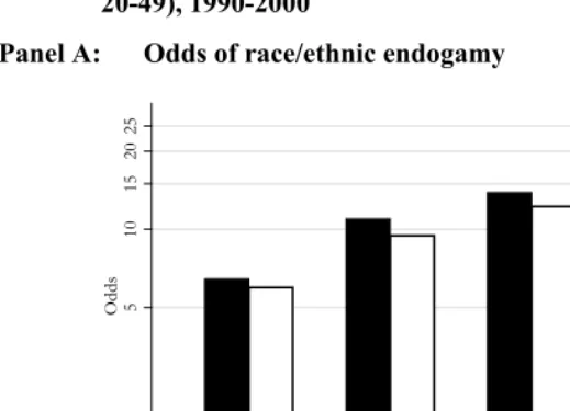
Panel A of Figure 1 shows the odds of race/ethnic endogamy by couple type and year. It shows striking evidence of a “gradient” in assortative matching, as was also evident in the descriptive statistics. Different-sex married couples are the most likely to be endogamous on race/ethnicity, followed by different-sex cohabiting couples, same-sex female couples, and lastly, by same-same-sex male couples. Table 3 shows that all of the differences by couple type are statistically significant at the 5% level, with the exception of the difference between same-sex male and female couples. Moreover, differences between same- and different-sex couples are quite large. For example, Panel A of Figure 1 shows that the odds of endogamy among same-sex male couples in 1990 were about 6:1. In other words, for every interracial/ethnic couple there were six endogamous couples, controlling for other variables. By contrast, the odds of endogamy among different-sex married couples were over 20:1. Column [1] of Table 3 shows the ratio of these odds. The ratio of the odds of endogamy for same-sex male couples compared with different-sex married couples in 1990 was 0.28 (6.34/22.55 = 0.28 as shown in Panel A of Figure 1). The smallest differences between same- and different-sex couples are those between same-different-sex female and different-different-sex cohabiting couples. Column [5] of Table 3 shows that the odds of race/ethnic endogamy among same-sex female couples were about 70% of the odds among different-sex cohabiting couples in both 1990 and 2000. Panel A of Figure 1 also shows that differences in assortative matching on race/ethnicity were remarkably stable between 1990 and 2000. The odds of endogamy decreased somewhat for all couple types except same-sex male couples, but these changes are quite small in comparison with the persistence of differences by couple type. Furthermore, none of the over-time changes in the contrasts between same- and different-sex couples are statistically significant.

(23)

was essentially equal to that for different-sex cohabiting couples in 1990 (Table 3, column [5]) but differences between same-sex female and different-sex cohabiting and married couples increased significantly between 1990 and 2000 (Table 3, columns [2] and [5]). These results are inconsistent with the hypothesis that differences in assortative matching between same- and different-sex couples have declined. Our findings suggest that differences in couple resemblance on age between same-sex female couples and different-sex cohabiting and married couples grew between 1990 and 2000.

Finally, Panels C and D of Figure 1 show the odds of crossing educational barriers by couple type and year. Panel C shows the odds of a match between high school graduates and college graduates. Panel D shows the odds of a match between more distant educational categories: those who have not completed high school and college graduates. Turning first to the odds of a match between high school and college graduates, we again see a strong pattern of assortative matching by couple type: sex male couples are the most likely to cross this educational divide, followed by same-sex female couples (in 1990 only), different-same-sex cohabiting couples, and different-same-sex married couples. Again, these differences are often large. In 1990, the odds of a union between a high school graduate and a college graduate among same-sex male couples were almost 60% higher than the odds for different-sex married couples and 45% higher than the odds for different-sex cohabiting couples (Table 3, columns [1] and [4]). These differences diminished in 2000, to 38% and 26%, respectively, but neither decline is statistically significant. Differences in assortative matching on education between same-sex female couples and different-sex couples also diminished, although again these declines are not statistically significant. In 1990 same-sex female couples were more likely than different-sex married and cohabiting couples to match across this educational divide (although the latter difference is not statistically significant) (Table 3, columns [2] and [5]), but were virtually indistinguishable from different-sex cohabiting couples in 2000 (Table 3, column [5]). Panel C also shows that the decline in the odds of educational intermarriage noted in previous studies (e.g., Schwartz and Mare 2005) was not limited to this group, but was a more general phenomenon occurring for all couple types.

(24)

The education results from the multinomial logit models differ somewhat from the descriptive statistics presented in Table 1, which showed that educational homogamy was similar among same-sex female and different-sex married couples, and among same-sex male and different-sex cohabiting couples. Separate analyses indicated that the homogamy results shown in Table 1 for same-sex male and female couples are inflated by the concentration of same-sex couples in the highest education categories. Controlling for these concentration effects, same-sex female couples are less likely to be educationally homogamous than different-sex married and cohabiting couples, and same-sex male couples are less likely to be educationally homogamous than all other couple types.

4.4 Assortative matching by couple type for couples aged 20 to 49

(25)

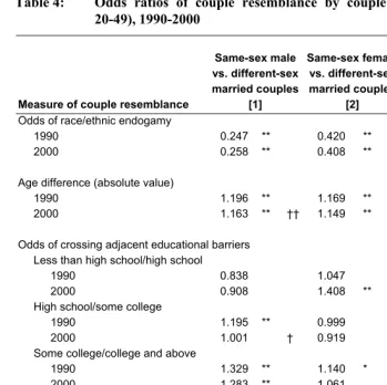
Table 4: Odds ratios of couple resemblance by couple type (couples aged 20-49), 1990-2000

Same-sex male vs. different-sex married couples

[1]

Same-sex female vs. different-sex married couples

[2]

Different-sex cohabiting vs.

different-sex married couples

1990 0.247 ** 0.420 ** 0.531 **

2000 0.258 ** 0.408 ** 0.529 **

1990 1.196 ** 1.169 ** 1.130 **

2000 1.163 ** †† 1.149 ** †† 1.098 ** ††

1990 0.838 1.047 1.259 **

2000 0.908 1.408 ** 1.328 ** ††

1990 1.195 ** 0.999 1.073 **

2000 1.001 † 0.919 1.065 **

1990 1.329 ** 1.140 * 1.069 **

2000 1.283 ** 1.061 1.037 ** †

1990 1.588 ** 1.139 1.148 **

2000 1.284 ** † 0.975 1.104 ** †

1990 1.330 1.192 1.444 **

(26)

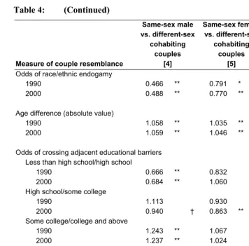
Table 4: (Continued)

Same-sex male vs. different-sex

[4]

Same-sex female vs. different-sex

[5]

Same-sex male vs. same-sex female couples

1990 0.466 ** 0.791 * 0.589 **

2000 0.488 ** 0.770 ** 0.633 **

1990 1.058 ** 1.035 ** 1.023 **

2000 1.059 ** 1.046 ** 1.012 *

1990 0.666 ** 0.832 0.800

2000 0.684 ** 1.060 0.645 **

1990 1.113 0.930 1.196

2000 0.940 † 0.863 ** 1.089

1990 1.243 ** 1.067 1.165 *

2000 1.237 ** 1.024 1.208 **

1990 1.383 ** 0.992 1.394 **

2000 1.163 ** 0.883 * 1.317 **

1990 0.921 0.825 1.115

2000 0.795 * 0.936 0.850

(27)

Figure 2: Measures of assortative matching by couple type (couples aged 20-49), 1990-2000

Panel A: Odds of race/ethnic endogamy

5

10

15

20

25

Odds

Same-Sex

Panel B: Odds of a match by the absolute value of the difference between partners’ ages

.7

5

.8

5

.9

5

1

Odds

Same-Sex

(28)

Figure 2: (Continued)

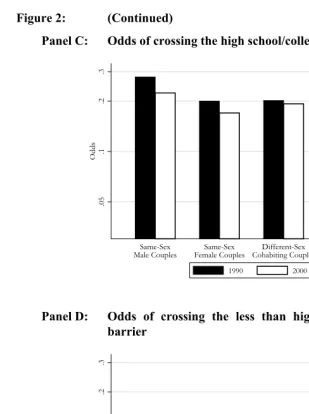
Panel C: Odds of crossing the high school/college and above barrier

.0

5

.1

.2

.3

Odds

Same-Sex

Panel D: Odds of crossing the less than high school/college and above barrier

.0

5

.1

.2

.3

Odds

Same-Sex

(29)

Finally, among couples aged 20 to 49, declining differences in educational homogamy between same- and different-sex married couples are somewhat more evident. The decline in the difference between same-sex male and different-sex married couples in the odds of partnership between high school graduates and college graduates is statistically significant (Table 4, column [1]). The difference in the odds of crossing this barrier between same-sex female couples and different-sex married couples also declined, although this change is not statistically significant. Overall, although there is somewhat more evidence of smaller differences in assortative matching on age and education in 2000 than in 1990 in the larger sample, substantial differences in matching patterns remain, especially for same-sex male couples. In addition, using the wider age range of couples, many of the differences in matching between same-sex male and female couples are now statistically significant, with same-sex male couples generally being less likely to resemble one another than same-sex female couples (Table 4, column [6]).11

5. Discussion

Same- and different-sex coresidential couples exhibit considerable positive assortative matching on age, race/ethnicity, and education. Nevertheless, there are large differences in matching by couple type, holding constant differences in couples’ background characteristics. In general, different-sex married couples tend to be the most likely to resemble one another, followed by different-sex cohabiting couples, same-sex female cohabiting couples, and finally by same-sex male cohabiting couples. These patterns hold for the majority of measures of couple resemblance.

Following Rosenfeld and Kim (2005), we expected differences in the matching patterns of same- and different-sex couples to have declined between 1990 and 2000 as the number of same-sex couples in the population has increased and as same-sex relationships have become more accepted. We found limited evidence to support this hypothesis. Differences in the odds of race/ethnic endogamy by couple type were remarkably persistent. Differences in the association between partners’ ages diverged somewhat by couple type for young couples, but lessened slightly for a wider age range

11_{Because the percentage increase in the number of same-sex couples in the U.S. was largest in Southern,}

(30)

of couples. By contrast, there is more consistent evidence of convergence in assortative matching on education. These changes did not attain conventional levels of statistical significance for couples aged 20 to 34, but were significant among couples aged 20 to 49. Among younger couples, convergence in educational assortative matching was large enough to completely eliminate the 1990 differences between same-sex female couples and different-sex cohabitors. These findings are consistent with the growing educational similarity of same- and different-sex couples in the U.S.

Caution must be exercised in the interpretation of our comparison of the 1990 and 2000 results, however, given changes in the U.S. Census Bureau’s procedure for handling same-sex couples who self-identified as married. It is clear that in 2000, a nontrivial proportion of same-sex couples are misclassified different-sex married couples (Black et al. 2007). To address this issue, we limited our analysis of same-sex couples to those who self-identified as “unmarried partners.” One potential consequence of limiting our sample in this way is that if an increasing proportion of homogamous same-sex couples self-identify as married, then the observed stability of differences in assortative matching by couple type may be due to the selection of homogamous same-sex “unmarried partner” couples into marriage. In other words, assortative matching among same-sex couples may have increased, but we may not observe this if homogamous couples are increasingly likely to identify themselves as married.

(31)

Other possible explanations for differences in couple resemblance include the diversity of the available pool of partners, geographic mobility, and differential selection out of unions. Same-sex couples are more likely to live in diverse neighborhoods than different-sex couples (Black et al. 2002; Gates and Ost 2004:35-36) and thus, gay men and lesbians may come into contact with partners with different characteristics than themselves more often than heterosexuals. Alternatively, because same-sex couples have higher levels of geographic mobility than different-sex couples, gay men and lesbians may not be subject to the same level of partner selection pressures from their friends and family as are heterosexuals (Rosenfeld and Kim 2005). Finally, like other studies that have relied on recent census data, we have examined a sample of prevailing unions and thus differential selection out of unions may affect our results. If dissimilar different-sex couples are more likely to split up than dissimilar same-sex couples, then differential selection out of unions may partially account for the differences in resemblance we observe (Schwartz forthcoming). Future research should investigate these explanations. As for future trends, whether differences in assortative matching between same- and different-sex couples persist depends on the extent of change in individuals’ preferences for partners and changes in partner availability.

6. Acknowledgements

(32)

References

Agresti, A. (2002). Categorical data analysis. New York: Wiley. doi:10.1002/0471249688.

Andersson, G., Noack, T., Seierstad, A., and Weedom-Fekjaer, H. (2006). The demographics of same-sex marriages in Norway and Sweden. Demography 43(1): 79-98. doi:10.1353/dem.2006.0001.

Black, D., Gates, G.J., Sanders, S., and Taylor, L. (2000). Demographics of the gay and lesbian population in the United States: Evidence from available systematic data sources. Demography 37(2): 139-154. doi:10.2307/2648117.

Black, D., Gates, G.J., Sanders, S., and Taylor, L. (2002). Why do gay men live in San Francisco? Journal of Urban Economics 51(1): 54-76. doi:10.1006/juec.2001.2237.

Black, D., Gates, G.J., Sanders, S., and Taylor, L. (2007). The measurement of same-sex unmarried partner couples in the 2000 U.S. census. Los Angeles: University of California: California Center for Population Research (Working Paper CCPR-023-07). http://www.ccpr.ucla.edu/ccprwpseries/ccpr_023_07.pdf.

Blumstein, P. and Schwartz, P. (1983). American couples: Money, work, sex. New York: William Morrow.

Carpenter, C. and Gates, G.J. (2008). Gay and lesbian partnership: Evidence from California. Demography 45(3): 573-590. doi:10.1353/dem.0.0014.

Casper, L.M. and Bianchi, S.M. (2002). Continuity and change in the American family. Thousand Oaks, CA: Sage Publications.

Cherlin, A.J. (2004). The deinstitutionalization of American marriage. Journal of Marriage and Family 66(4): 848-861. doi:10.1111/j.0022-2445.2004.00058.x. DiPrete, T.A. (1990). Adding covariates to loglinear models for the study of social

mobility. American Sociological Review 55(5): 757-773. doi:10.2307/2095870. Gates, G.J. (2006). Same-sex couples and the gay, lesbian, bisexual population: New

estimates from the American Community Survey. Los Angeles: The Williams Institute. http://www.gaydata.org/02_Data_Sources/ds029_ACS/ SameSexCouplesandGLBpopACS.pdf.

(33)

Gates, G.J. and Ost, J. (2004). The gay and lesbian atlas. Washington, DC: The Urban Institute.

Gates, G.J. and Sell, R. (2007). Measuring gay and lesbian couples. In: Hofferth, S.L. and Casper, L.M. (eds.). Handbook of measurement issues in family research. Mahwah, NJ: Lawrence Erlbaum Associates: 235-244.

Hamplova, D. (2009). Educational homogamy among married and unmarried couples in Europe: Does context matter? Journal of Family Issues 30(1): 28-52. doi:10.1177/0192513X08324576.

Harry, J. (1984). Gay couples. New York: Praeger.

Hayes, A.F. (1995). Age preferences for same- and opposite-sex partners. The Journal of Social Psychology 135(2): 125-133. http://www1.appstate.edu/~kms/classes/ psy2664/Documents/Hayes1995.pdf.

Hertzog, M. (1996). The lavender vote: Lesbians, gay men, and bisexuals in American electoral politics. New York: New York University Press.

Jepsen, L.K. and Jepsen, C.A. (2002). An empirical analysis of the matching patterns of same-sex and opposite-sex couples. Demography 39(3): 435-453. doi:10.1353/dem.2002.0027.

Joyner, K. and Kao, G. (2005). Interracial relationships and the transition to adulthood. American Sociological Review 70(4): 563-581. http://www.jstor.org/stable/4145377.

Knoke, D. and Burke, P.J. (1980). Log-linear models. Sage university paper series on quantitative applications in the social sciences, Vol. 20. Beverly Hills, CA: Sage Publications.

Kurdek, L.A. (2003). Differences between gay and lesbian cohabiting couples. Journal of Social and Personal Relationships 20(4): 411-436. doi:10.1177/02654075030204001.

Kurdek, L.A. (2006). Differences between partners from heterosexual, gay, and lesbian cohabiting couples. Journal of Marriage and Family 68(2): 509-528. doi:10.1111/j.1741-3737.2006.00268.x.

(34)

Loftus, J. (2001). America’s liberalization in attitudes toward homosexuality, 1973 to 1998. American Sociological Review 66(5): 762-782. doi:10.2307/3088957. Logan, J.A. (1983). A multivariate model for mobility tables. American Journal of

Sociology 89(2): 324-349. doi:10.1086/227868.

Mare, R.D. (1991). Five decades of educational assortative mating. American Sociological Review 56(1): 15-32. doi:10.2307/2095670.

Meier, A., Hull, K.E., and Ortyl, T.A. (2009). Young adult relationship values at the intersection of gender and sexuality. Journal of Marriage and Family 71(3): 510-525. doi:10.1111/j.1741-3737.2009.00616.x.

Ortyl, T.A., Hull, K.E., and Meier, A. (2009). Attitudes toward union formation at the intersection of gender and sexual identity. Paper presented at the annual meetings of the Population Association of America, Detroit, May 2009.

Over, R. and Phillips, G. (1997). Differences between men and women in age preferences for a same-sex partner. Behavioral and Brain Sciences 20(1): 138-140. doi:10.1017/S0140525X97220042.

Phua, V.C. and Kaufman, G. (1999). Using the census to profile same-sex cohabitation: A research note. Population Research and Policy Review 18(4): 373-386. doi:10.1023/A:1006234713127.

Pollard, M.S. and Harris, K.M. (2007). Measuring cohabitation in add health. In: Hofferth, S.L. and Casper, L.M. (eds.). Handbook of measurement issues in family research. Mahwah, NJ: Lawrence Erlbaum Associates: 35-51.

Powers, D.A. and Xie, Y. (2000). Statistical methods for categorical data analysis. 1st edition. San Diego: Academic Press.

Qian, Z. and Lichter, D.T. (2007). Social boundaries and marital assimilation: Interpreting trends in racial and ethnic intermarriage. American Sociological Review 72(1): 68-94. http://www.ingentaconnect.com/content/asoca/asr/2007/ 00000072/00000001/art00004.

Raftery, A.E. (1995). Bayesian model selection in social research. Sociological Methodology 25: 111-163. doi:10.2307/271063.

(35)

Rosenfeld, M.J. (2008). Racial, educational, and religious endogamy in the United States: A comparative historical perspective. Social Forces 87(1): 1-32. doi:10.1353/sof.0.0077.

Rosenfeld, M.J. and Kim, B. (2005). The independence of young adults and the rise of interracial and same-sex unions. American Sociological Review 70(4): 541-562. http://www.jstor.org/stable/4145376.

Ruggles, S., Sobek, M., Alexander, T., Fitch, C.A., Goeken, R., Hall, P.K., King, M., and Ronnander, C. (2004). Integrated public use microdata series: Version 3.0 [electronic resource]. Minneapolis, MN: Minnesota Population Center. http://usa.ipums.org/usa/.

Schaffner, B. and Senic, N. (2006). Rights or benefits? Explaining the sexual identity gap in American political behavior. Political Research Quarterly 59(1): 123-132. doi:10.1177/106591290605900111.

Schwartz, C.R. (Forthcoming). Pathways to educational homogamy in marital and cohabiting unions. Demography.

Schwartz, C.R. and Mare, R.D. (2005). Trends in educational assortative marriage from 1940 to 2003. Demography 42(4): 621-646. doi:10.1353/dem.2005.0036. Seltzer, J.A. (2000). Families formed outside of marriage. Journal of Marriage and

Family 62(4): 1247-1268. doi:10.1111/j.1741-3737.2000.01247.x.

Seltzer, J.A. (2004). Cohabitation and family change. In: Coleman, M. and Ganong, L.H. (eds.). Handbook of contemporary families: Considering the past, contemplating the future. Thousand Oaks, CA: Sage Publications: 57-78.

Simkus, A. (1984). Structural transformation and social mobility: Hungary 1938-1973. American Sociological Review 49(3): 291-307. doi:10.2307/2095275.

Smits, J., Ultee, W., and Lammers, J. (1998). Educational homogamy in 65 countries: An explanation of differences in openness using country-level explanatory variables. American Sociological Review 63(2): 264-285. doi:10.2307/2657327. Smock, P.J. (2000). Cohabitation in the United States: An appraisal of research themes,

findings, and implications. Annual Review of Sociology 26:1-20. doi:10.1146/annurev.soc.26.1.1.

(36)

Appendix:

The relationship between multinomial logit and log-linear models

In what follows, we outline the relationship between the multinomial logit models used in this paper and log-linear models. Our discussion relies heavily on Agresti’s more detailed treatment of this issue (Agresti 2002:330-332).

For simplicity, consider a multinomial logit model in which we are only interested in differences in race/ethnic matching by couple type. A multinomial logit model similar to that presented in equation (2) but considering only race/ethnic matching and the race/ethnic characteristics of partners is:

(

)

(

1 2

)

1 2

,

log 2,..., 4

1 ,

R

R R O

j jk jl j

P Y j R k R l

j

P Y R k R l α β β δ

= = =

= + + + =

= = = (A1)

where Y denotes couple type (j=1,…,4; different-sex married, different-sex cohabiting, same-sex female, same-sex male) and different-sex married couples are the baseline category, R1 and R2 are partner 1 and 2’s race/ethnicity (k,l=1,…4), and OR is a race/ethnic endogamy term.12

A log-linear model that produces coefficients and standard errors equivalent to those in equation (A1) can be written as:

( )

1 2 1 2 1 2

log Y R R R R R Y R Y O YR

jkl j k l kl kj lj j

μ = +λ λ +λ +λ +λ +λ +λ +λ (A2)

In fitted marginals notation (Knoke and Burke 1980), equation (A2) can be written as [R1R2] [R1Y] [R2Y] [ORY]. To see the equivalency between the log-linear and multinomial coefficients, we can calculate the log odds of being in couple type j versus type J, which is the dependent variable in equation (A1), using the log-linear model equation. In this example, we compare same-sex male couples (j=4) to different-sex married couples (j=1):

12_{Partner 1 is males in different-sex relationships and household heads in same-sex relationships. Partner 2 is}

(37)

(

)

(

)

(

)

( )

(

)

(

)

(

)

(

) (

)

1 2 1 2 1 2

1 1 2 2

1 2 ₄

4 1

1

1 2

4 4 4 4

1 1 1 1

4 1 4 1 4 1 4 1

4 ,

log log( ) log log

1 , . R R R R kl kl kl kl

R R R R R Y R Y O Y

Y

k l kl k l

R R R R R Y R Y O Y

Y

k l kl k l

R Y R Y R Y R Y O Y O Y

Y Y

k k l l

P Y R k R l

μ _μ _μ μ λ λ λ λ λ λ λ λ λ λ λ λ λ λ λ λ λ λ λ λ λ λ λ λ = = = = = − = = = = + + + + + + + − + + + + + + + = − + − + − + −

In the last line of the equation above, the first parenthetical term is the constant in the multinomial logit model for same-sex male couples relative to different-sex married couples (

α

₄) and is equal to in equation (A2) when different-sex married couples are the omitted category. The second parenthetical term represents the association between partner 1’s race/ethnicity and the log odds of being a same-sex male couple versus a different-sex married couple, which is in equation (A1) and in equation (A2). Similarly, the third parenthetical term is equal to in equation (A1)

and in equation (A2). Finally, the fourth parenthetical term is the difference in the log odds of endogamy for same-sex male couples versus different-sex married couples, which is equal to in equation (A1) and in equation (A2). Note that the log-linear model contains all possible interactions between variables not involving couple type and their lower-order terms ( , , ) and that these terms cancel when taking the difference in logarithms.

Y

4

Y R k14

λ

2 4 R l

β

Y R l42

λ

R O 4

δ

λ

1 4 R k

β

Y OR 4

λ

1 R2

l

λ

2 1R R kl

λ

R k

λ

The multinomial logit models used in this paper are more complex, but the same principles apply. Written in fitted marginals notation, the log-linear equivalent of equation (2) is

[R1R2A1A2E1E2T] [R1YT][R2YT][A1YT][A2YT][E1YT][E2YT][ORY][OAY][OEY]

(38)

coefficients to vary over time (i.e., [ORYT][OAYT][OEYT]). The exponentiated time-varying δ’s from Model E1 appear in Tables 3 and 4.