Approximate Solution of Sensitivity Matrix of Required Velocity Using Piecewise Linear Gravity Assumption

© Iranian Aerospace Society, Summer - Fall 2012

J

Journal of Aerospace Science and Technology

A S T

1 Introduction

Required velocity and its sensitivity matrix are well-known concepts in space applications. The required velocity is a hypothetical instantaneous velocity for a only under gravitational acceleration. Depending on -ative of the required velocity with respect to position vector [1-5].

The analytical solutions of the required velocity and its sensitivity matrix have been obtained for ! "#$% analytical/explicit solution could not be obtained for algorithms have been developed for the problem.

The well-known Q-guidance scheme presented in &"#$ ' ( "#$ )*+46(% 7 "8$

( '7 "6$

A lot of research can be found in the literature for the few works are available for the second required velocity "4$% : -turbation techniques and time-varying gravity ; -ate approach to deal with a group of nonlinear problems "+*#$

) ' been presented using linear gravity assumption along -"*<$= problem and must be obtained for the solution. Higher accuracy levels can be achieved using piecewise present work.

Approximate Solution of Sensitivity Matrix of Required Velocity

Using Piecewise Linear Gravity Assumption

%=> ?

1

In this paper, an approximate solution of sensitivity matrix of required velocity

time.

2 Basic Formulation

Consider a spacecraft modeled as a particle P moving only under gravitational acceleration. The governing

equation of motion isv g r( );where rv g are

-tively; and the overdot represents the differentiation with respect to time t. Integrating the preceding relation twice yields:

v( )t v g r( ( ))d

t t

= 0+

_∫

0

Y Y (1a)

r( )t r (t t)v (t ) ( ( ))g r d

t t

= + −0 0 0+

_∫

− 0

Y Y Y (1b) LMO the position and velocity at an arbitrary time t k > t0 are

given by:

(2a)

v( )t_k v g r( ( ))t dt

t tk

= 0+

_∫

0

r( )t_k r (t_k t )v (t_k t) ( ( ))g rt dt t

t_k

= +0 − 0 0+

_∫

−

0

(2b)

U t_f tk is replaced by tf.

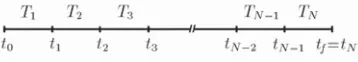
The above equations are not integrable in the current [ , ]t t0 _f is divided into N

sub-intervals of [ ,t t_{j j}1] having time length of Tj+1=tj+1−tj

for j=0 1, , ,…N−1(see Fig.1). An approximate solution can be found using linear gravity assumption for each interval of [ ,_{t t} ]

j j1

W#X

g r( ( ))t t t g r( ( )) g r( ( ))

t t t

t t

t t t

j

j j

j

j

j j

j

= −

− +

− −

+

+ + +

1

1 1

1

= between two or more points may be selected. This is -tional burden.

Figure 1. Time intervals representation.

3 Linear Approximation of Velocity

The integral part of Eq. (2a) may be broken down into the summation of integrals:

v

( )

t

_f

v

g r

( ( ))

t dt

t

t

j N

j j

=

+

+

∫

∑

₌−

0 0

1

1

(4)

% \W#X integration results in

v( )_t v _Tg _T g (_{T T} )g _N

f N N j j j

j N

= + + + + + ≥

= −

∑

0 1 0 1

1 1 1

2 1 2

1

2 for 2 (5)

where gj stands for g r( ( ))t_j .

U (Tj T)we

have:

0 0 1 1

1

( ) ( 2 2 )

2

f N N

t T

v v g g " g g _W8X

To obtain gj^

the position vectors at the time t_j’s must be

approxi-mated.

4 Linear Approximation of Position

\W@X is written in the following summation form:

r r v g r

k k _t k

t

j k

t t t t t dt

j j

= + − + + −

∫

∑

₌−

0 0 0

0 1

1

( ) ( ) ( ( )) (7)

where rk denotes r( )tk . Using the piecewise linear

W#X `

(t_k t) ( ( ))t dt T [ (t t ) T ]

t t

j k j j j

j j

− = − +

+

∫

g r + + + g

1 1

6 13 1 2 1

(8)

+ Tj+[ 1

6 13((tk−tj)−2Tj+1]gj+1

We can thus write (2 k N)

6 1 3 2

0 1

1 1 1 0

2

(t t) ( ( ))t dt T[ (t t ) T]

T

k t

t

j k

k

k k j j

j

− = − +

+ +

+

∫

∑

₌−

=

g r g

g 11 1

2 1 2

1 3

k

j j j j k j j

T T T T t t

−

+ +

∑

[ − + ( + )( − )]g (9)

For k 1 we have

r₁ r_{0 1 0}v ₁2 g g

0 1

1

6 2

= +T + T ( + )

(10)

) `

t

_k

− = −

t

_j

(

k

j T

) , for 0

≤ < ≤

j

k

N

(11)

\W+X (2 k N):

t

0

r₁ r₀ 1 ₀ v g_{0 0} 2

2

3 8

= + ₍ − ₎ ∗− ₍ − ₎

t_f t _f t_f t (19)

r

₂

r

_{0 0}

v

1

g

_{0 0} 2

2

= +

₍

−

₎

∗

−

₍

−

₎

t

_f

t

_f

t

_f

t

(20)

3

g_i Nr_j /r_j , (j 0,1,2) (21)

v∗_v( )t0 =v∗_f − (g0+ g1+g2)(t_f−t0) 1

4 2 (22)

where rj |rj | and N is the Earth gravitational constant.

As can be seen in Eq. (21), the spherical Earth model is used here; however, elliptical Earth model can also be utilized in the formulation.

b) Four-point approximation

The algorithm for three-equal intervals is extended as follows:

r₁ r₀ 1 ₀ v g_{0 0} 2

3

5 18

= + ₍ − ₎ ∗− ₍ − ₎

t_f t _f t_f t (23)

r₂ r₀ 2 ₀ v g_{0 0} 2

3

4 9

= + ₍ − ₎ ∗− ₍ − ₎

t_f t _f t_f t (24)

r₃ r_{0 0} v 1g_{0 0} 2

2

= +₍ − ₎ ∗− ₍ − ₎

t_f t _f t_f t (25)

3

g_{i N}r_j/_rj , (_j0,1,2, 3)

(26)

v∗_v( )t0 =v∗_f − (g0+ g1+ g2+g3)(t_f−t0)

1

6 2 2 (27)

6 Sensitivity Matrix with Velocity Constraint

( ) ( ) / ( )

v v

Q t vt rt. Here, we assume that t0

is the current time, so we calculate Qv v( ) /t0 0

v r. By

taking the partial derivative of Eq. (14) with respect to position r0 we have(N2)

∂

∂ = −

∂

∂ +

∂ ∂ ⎛

⎝ ⎜⎜⎜ ⎜

⎞ ⎠ ⎟⎟⎟

⎟⎟− +

∗

+

v r

g r

g r v

N N

j j j

t

T T T T

( )

( )

0

0

1 0

0 0

1

1 2

1 2 ₌₌

−

∑

₁1 ∂_∂

0

N

j g r (28)

Using the relation of

∂

∂ = − ⎡⎣⎢ − ⎤⎦⎥ ∂ ∂ g

r u u

r r

j

j

rj rj

T j

r I

0 3

0

3

r

(29)

(12)

6

2 1 1

(

T

j k

+

∑

= −

kk−j)g_j

5 Required Velocity with Velocity Constraint

desired velocity of v_f under gravity acceleration in a

tf is denoted byvv

. Without loss of generality, we formulate the problem for v_v( )t0 .

Using Eq. (1a) the required velocity v_v( )t0 is given by:

v_v v_f g r _{v v}

t t

t

t dt

v f

∗ ∗

=

= −

∫

∗

( )₀ [ (t) | _{( )}]

0 0

0

(13)

Using piecewise linear approximation results in:

v v g g g

v f N N j j

j N

j

t T T T T

∗ ∗

+ =

−

= − + −

∑

+

( )₀ ( _{1 0} ) ( ₁)

1 1

1 2

1 2

(14)

U `

v_v∗( )t0 =v∗_f − T(g0+ g1+ + g_N−1+g_N) 1

2 2 " 2 (15)

; g_j’s

or rj’s are to be calculated. Several approaches may be

utilized for this purpose. The simplest method is that,

r_k is calculated for constant gravity assumption; that is,

r( )t = + −r0 (t t0) ( )v_v∗ t0 + g0(t−t0) 2 1

2 (16)

Substitution of v∗_v( )t0 =v∗_f−g0(t_f−t0) into the preceding relation yields:

r( )t = + −r (t t )vf + g[(t−t )− (tf −t )](t−t )

∗

0 0 0 0 0 0

1

2 2 (17)

Therefore,

r_k = + −r0 t_k t0 v∗_f+ g0 t_k−t0 − t_f−t0 t_k−t0

1

2 2

( ) [( ) ( )]( ) (18)

a) Three-point approximation

In the case of three-point approximation, there are two

intervals (_N2). Therefore, based on the mentioned

by:

6 1 3 1

0 1

2

0 2

(_{tk t}) ( ( ))_{t dt T} ( _k ) _T

t t

j k

k j

j

− = − +

+

∫

∑

= −

g r g g

g_j

g_j

one can obtain:

2 _{1 0}

0

1 1

1

0

Q_v T F T F_{N N} N T T F

j j

j N

j j

= + ∂

∂ + +

∂ ∂ + =

−

∑

r r

r r

( ) (30)

where I is a 3 3 identity matrix, u_rj r_j /r_j, and

(31)

Therefore,

0 0

j j

j F

g r

r r (32)

In the case that we utilize Eq. (18) for approximation of

r_k , we have

(33)

Hence, substitution for rk/r0from the preceding rela-tion into Eq. (30) results in:

2 1

2

1 0 0 0

2

1 1

1

Q_v T F T F_{N N} T F F t_{N N f} t T_j T_j F j

N

j

= + + − + + +

= −

∑

( ) ( ) (34)

1

2 Tj Tj

− ( + ₊₊

= −

∑

1 − − − −

1 1

0 0 2 0 0

)( )[( ) ( )]

j N

j j f i

t t t t t t F F

Special Case: Fixed-time interval

) \W#<X

(N 2):

(2 ) 1( )

2 2

0 0 0

1 1 N Qv H HN tf t H HN Hj

j N

= + + − +

= −

∑

₍₃₅₎

( ) ( )

1

2

2 0

1 N tf t j N j

N

+ − −

= − −

∑

1 jH Hj 0

where

0 3

( )

3

f T

j rj rj

j

t t

H I

r

N

u u _!

(36)

The solution is now given for several values of N as

follows:

a) Two-point approximation (N 1):

2 1

2

0 1 0 1 0

Q_v =H +H + (t_f−t H H) (37)

b) Three-point approximation(N 2):

(38)

c) Four-point approximation (N 3):

6 2 2 1

2

0 1 2 3 0 3 0

Q_v =H + H + H +H + (t_f −t H H)

(39)

5 9

8 9

0 1 0 0 2

tf t H H tf t H H

+ ( − ) + ( − ) ₁₁

7 Simulation Results

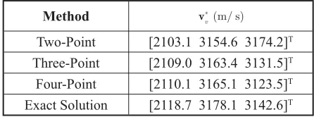
First, the obtained approximate solutions of the re-quired velocity are compared to each other and to the ! simulation for the spherical-Earth model. The initial

position of the vehicle is given as[0 0_R]

e

T_{; whereR}

e

\ is [2 3 0 5. ]T_{km/s in the Earth-Centered Inertial (ECI)}

coordinates. The required velocity of the vehicle at its ! #MM is vv

T

∗_{=[2118 7 3178 1 3142 6. . . ]}

m/s, obtained using nonlin-! required velocity are also obtained using two-, three-, and four-point approximations and the results are listed in Table 1. As can be seen, three-point approximation has better accuracy than two-point approximation, but its results are relatively similar to the four-point ap-proximation. Since, the midpoint positions have been obtained using constant gravity assumption, increasing the number of midpoints from 3, would not necessarily result in higher accuracy. To achieve a better result, the accuracy of the midpoint positions must be increased and that could be obtained by the present method.

Table 1. Calculation of required velocity for tf300s.

Method vv

_{(m/ s)}

Two-Point [2103.1 3154.6 3174.2]T

Three-Point [2109.0 3163.4 3131.5]T

Four-Point [2110.1 3165.1 3123.5]T

Exact Solution [2118.7 3178.1 3142.6]T

Next, the approximate solutions for sensitivity matrix with velocity constraint are evaluated. Here, a vertical planar motion in the spherical-Earth model is consid-ered. The vehicle nominal trajectory is given by

2

cos( / 3) 4.73

I e

x R Q t

2

sin( / 3) 8.87

I e

z

R

Q

t

(40b)

where ( , )x zI I are the ECI coordinates.

(40a)

3 3

T j rj rj

j

F I

r

N

u u _!

0 0 0 0

0

1_{( )[( ) 2( )]}

2 k

k k f

I t t t t t t F

r r

0 1 2 0 2 0 0 1 0

1 3 4 2 ( ) ( )

2 4

v f f

Q H H H t t H H t t H H

(a)

(b)

(c)

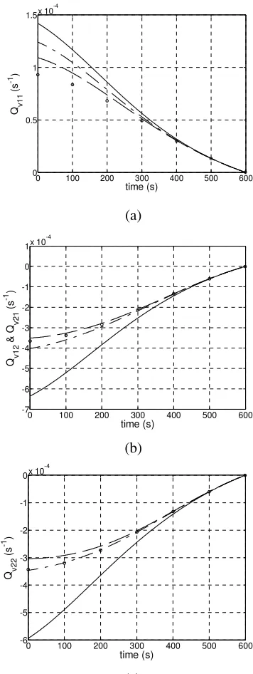
Figure 2. Different solutions of Q_v elements for tf300s; solid-line:

2-point approximation, dash-dotted line: 3-point approximation, dashed-line: 4-point approximation, and circles are the numerical

(b) (b)

( c)

Figure 3. Different solutions of Qv elements fortf300s

(line representations are similar to Fig. 2).

U @#

solutions for Q_v elements at t_f 300 8MM

)

solution (N 1) (N 2)

and four-point approximation (N3) are shown by solid

)

∆vv ∆r

∗_/

using

! ; ƒ

all the solutions have adequate accuracy for tf 300s.

U U #

c for t_f 300s. The accuracy of the four-point solution

(a)

0 100 200 300 400 500 600 -7

-6 -5 -4 -3 -2 -1 0 1x 10

-4

time (s)

Qv1

2

& Q

v2

1

(s

-1)

(b)

0 100 200 300 400 500 600 -6

-5 -4 -3 -2 -1

0x 10

-4

time (s)

Qv2

2

(s

-1 )

(c)

0 100 200 300 400 500 600 0

0.5 1 1.5x 10

-4

time (s)

Qv1

1

(s

-1)

0 50 100 150 200 250 300 0

0.2 0.4 0.6 0.8

1x 10

-4

time (s)

Q v11

(s

-1)

(a)

0 50 100 150 200 250 300 -4.5

-4 -3.5 -3 -2.5 -2 -1.5 -1 -0.5

0x 10

-4

time (s)

Qv1

2

& Q

v2

1

(s

-1)

(b)

0 50 100 150 200 250 300 -4

-3.5 -3 -2.5 -2 -1.5 -1 -0.5

0x 10

-4

time (s)

Qv22

(s

-1)

the reason for which has been explained earlier. The re-sults are case-dependent and approximate solutions need ! can also be enhanced using correction factors as treated &"*<$ = ! of midpoints may also be increased and that could be obtained by the present method.

;

-trix Q_v„

; give accurate approximation for onboard calculations ; ' calculations of Q_v and their accuracies and computational burden can be compared.

8 Conclusions

This work presented an analytical solution for sensi-tivity matrix using piecewise linearization of ! The method has been utilized to derive an approximate -straint. The accuracy of the method can be enhanced by a trade-off between accuracy and onboard computation-al burden. The method can be applied to ellipticcomputation-al Earth

Appendix: Sensitivity Matrix with Position Constraint

) U „ "<$ƒ ( ……4&"#$

added that “The corrected version is courtesy of

„&†%'‡ˆ-ratory.”

Using Eq. (1b) we can write

(41)

-sition r_f

position constraint and is denoted by v_{p. Using the} pre-ceding relation we have:

(42)

‰ \ W#X gives:

6 _{0 0} 6 _{0 1}3 _{0 1 0}

2 2

( ) ( ) ( ) [ ( ) ]

[

t t t T t t T

T T T

f p f f

N f j j

− = − − − −

− − −

∗ ∗

+

v r r g

g 2₁₁

1 1 1 3 + + ₊ − = −

∑

(_{Tj Tj} )(_{tf tj})] j

N

j

g W<#X

Partial differentiation with respect to position vector results in:

6 ₀ 0 6 3

0

1 0 1 0

(t_f t ) p( )t I T[ (t t) T F] f

− ∂

∂ = − + − −

∗

v

r (44)

3

2 1 2

[T_j T_j (T_j

+ − ₊ + +TT_j t t F

j N

f j j j + = −

∑

− ∂ ∂ 1 1 1 0

)( )] r

r

where Fj \W#*X

T=(t_f −t0) /N`

v_p rf r g g g f f f j N j t t t t t

N N N j

∗ ∗ = − = − − − − − + + − ⎧ ⎨ ⎪

∑

( )₀ 0 ( ) ( )

0 0

2 0

1 1

6 ⎪⎪_⎩⎪⎪3 1 6

⎫ ⎬ ⎪⎪ ⎭⎪⎪(45) W<8X ∂ ∂ = −− + − _{+ −} ∂ ∂ ∗ = −

∑

v r r r p f j N j j t _I t t N

N H N N j H

( )

( )

0

0 0

2 0 2

1 1 0 3 1 6 1

where H_i =(t_f −t F0) _i.

‡

approximation must be selected for / ₀

j

r r. For

\W6X(N2) we obtain:

r_k r _k v_p k

f

f k

t t t t

t t t t

= + − + − −

{

− ∗ 0 0 0 2 0 6 3 ( ) ( )

( ) [ ( ) ₍₄₇₎

g

k

t t

+2( − 0)] 0 +(ttk −t0)gf

}

2 0

0 3 0 0

0 0

( )

( ) ( )(3 )

6 p k f f t k k

I t t t t N k H

N N v r

r r (48)

% \ W<4X \ W<8X -ment results in:

(49)

1

1

0 0 0

0

( ) ( ) j ( ) ( ( ))

j

N _t

f f _t f

j

t t t t t t dt

*,

r r v g r

1 1 0 0 0 0 0 1

( ) j ( ) ( ( ))

j

N _t

f

p _t f

j

f f

t t t t dt

t t t t

* ,

r r

v g r

1 1 0 0 3 1 0 ( ) ( ) N p f j j

t t t

where

J

t t I

N

N H N N j H

f j

N

j

= −

− +

− _{+ −}

= −

∑

1 3 1

6

1

0

2 0 2

1 1

( ) (50)

t t

N N j

f

j N

+ − −

= − 6

0 5

1 1

( )

∑

∑

(3 − )2

0 N j j H H_j

The sensitivity matrix p( ) /t0 0

v r in the right-hand

side of Eq. (48) may also be replaced by a three or more-point approximation in order to obtain a more

References

1. ‰ Š & ) Š > ‹ Œ %)?'W*+8@X

2. ( &=L%Š \ ? OJournal of Guidance, Control, and Dynamics…W@X‰‰+6**MW*+4@X

# ( &=;) „ „ ; & \ ;);;\ % ‘%;W*+++X

4. „ U = †ˆ ?’ † % „ ‡% „) † „;‘%;W*+8…X

5. % Š„„ Š †%-% “)?W@MM<X

8 („%% %”L;’ 7Š % % ˆ “ -OJournal of Guidance, Control, and

Dynam-ics*MW*X‰‰…#8MW*+46X

7. > ? %=L;) Š

“ † O)

/'1;\&’

@M*M#*MM)W@M*MX

8. > ? %=L‡ \ %

„ U “ † O

' )

;% 8W@X‰‰……8*W@MM+X

9. & > ) L‰ ˆ : „ ) “‰ ’ % O

$ ' # 1

*4*‰‰*@#*<8W@MM8X

10. = ‡ Š = † L? \Š % ‰ ˆ

-†O ')

1-ference#’UˆW*++*X

11. =‡Š?'„>L?

†“ Š O''2'''

" 1 ?+#@@M** ‰

†;W*++#X

12. &>)L‡ ‰ ’ ? ’ „‰ ˆ

: „O1 3"

@4‰‰*#M8*#*#W@MM8X

*# („;‡‡(’ „ ‹ L; ‰ ˆ † ; & ˆ “ Š †OThe 14th Mediterranean Conference

1 'W@MM8X

14. > ? %=L; % „ U “ † ˆ “ Š ; O

6 3 <W#Œ<X