RESEARCH PAPER
Numerical Simulation of a Lead-Acid Battery Discharge
Process using a Developed Framework on Graphic
Processing Units
Hossein Mahmoodi Darian*
School of Engineering Science, College of Engineering, University of Tehran, Tehran, Iran
Received: 4 January 2019, Revised: 19 March 2019, Accepted: 23 April 2019 © University of Tehran 2019
Abstract
In the present work, a framework is developed for implementation of finite difference schemes on Graphic Processing Units (GPU). The framework is developed using the CUDA language and C++ template meta-programming techniques. The framework is also applicable for other numerical methods which can be represented similar to finite difference schemes such as finite volume methods on structured grids. The framework supports both linear and nonlinear finite difference stencils. Furthermore, the arithmetic operators and math functions are overloaded to ease the array-based computations on GPUs. The reduction algorithms are also efficiently included in the framework. The discharge process of a lead-acid battery cell is simulated using the facilities provided by the framework. The governing equations are unsteady and include two nonlinear diffusion equations for solid (electrode) and liquid (electrolyte) potentials and three transient equations for acid concentration, porosity and the state of charge. The equations are discretized using the finite volume method. The framework allows the user to develop the numerical solver with a few efforts. The numerical simulation results are reported for different relations for open circuit potential and the electrolyte diffusion coefficient.
Keywords: CUDA,
Discharge Process, Finite Difference Method,
Finite Volume Method, Graphics Processing Units,
Lead-Acid Battery
Introduction
Using Graphics Processing Units (GPU) for numerical simulations has become popular in the scientific and engineering areas. Nowadays, high-end GPUs have several thousand computing cores that means they can simultaneously compute several thousand mathematical operations. The CUDA language is the most popular programming language for parallel processing using GPUs. However, due to the more complex structure of parallel programming and less debugging facilities, the development of a GPU numerical simulation code is a time-consuming task. In the present study, we developed a framework for using finite-difference schemes on GPUs. The framework includes several classes for defining array objects, mathematical expressions and finite difference schemes on the GPU device. The framework also includes
* Corresponding author
several functions, which allows the user to easily implement loops for array computations. Another advantage of the present framework is that the reduction algorithms (i.e. computing the minimum, maximum or sum of the array elements) are efficiently implemented and the user can easily utilize them. It should be mentioned that the framework is also applicable for other numerical methods which can be represented similar to finite difference schemes such as finite volume methods on structured grids.
Due to the complexity of batteries, modeling and simulation are useful tools to optimize and analyze behavior and a better understanding of physical phenomena. Simulating the discharge process is important which enables researchers to predict the voltage drop of the battery cell as a function of time. The developed framework is utilized to simulate the discharge process of a lead-acid battery cell on a GPU. The model consists of unsteady nonlinear one-dimensional diffusion equations, which discretized using the finite volume method. The equations model the dynamic behavior of acid concentration, the porosity of the electrodes and the state of charge (SoC) of the cell. At each time step, an iterative algorithm solves the nonlinear system of equations. The results are validated by the previous works and presented for different empirical relations for the open circuit potential and the electrolyte diffusion coefficient.
Framework
To utilize the GPU cores in CUDA, one must write a GPU device function (or simply a kernel). This means even for a simple arithmetic operation; the user must write a kernel. In the present framework, using the C++ templates meta-programming techniques [1-3], which also supported by CUDA 7.0 and later versions, and overloading the arithmetic operators and math functions, the compiler automatically produces the required kernels (hidden from the user). For instance, in the following code, three arrays are defined and allocated on GPU memory with a size of 100 elements and then some operations are accomplished on:
#include <iostream> #include <algorithm> #include "exprNew.h" #include "stencilExpr.h" #include "cuarr.hpp" #include "cuMakePatch.hpp" #include "Stencil.hpp" #include "Reduce.h" #include <cmath>
using namespace std;
int main(int argc, char *argv[]) {
int N = 100;
cuarr<double> X;
cuarr<double> Y;
cuarr<double> T;
X.Alloc(N); Y.Alloc(N); T.Alloc(N);
X = 3.1415926; Y = 2 * X;
T = sin(X + Y);
The files "exprNew.h", "stencilExpr.h", "cuarr.hpp", "cuMakePatch.hpp", "Stencil.hpp", and "Reduce.h" includes all the framework classes and functions definitions. In the above code, the three lines before “return 0” calculates some operations. The compiler produces and executes a kernel for each of the lines. As observed, the user writes a simple code and the compiler accomplishes the other time-consuming tasks.
Finite Difference Schemes
The framework provides two methods for defining finite difference operators. One is only suitable for linear schemes while the other method is suitable for both linear and nonlinear schemes.
A suitable way to express a linear stencil is to express it by the pairs of the (non-zero) coefficients and the corresponding distance from the base index. For instance, the central scheme for the first derivative can be expressed as:
1
2ℎ𝑓𝑖+1− 1
2ℎ𝑓𝑖−1 → ( 1
2ℎ, 1) (− 1
2ℎ, −1) (1)
The framework allows the user to define and apply this scheme as:
Stencil1D<2> CentralSchemeStencil (1, 1/(2*h),-1, -1/(2*h));
FiniteDifferenceOperator<2> CentralScheme;
CentralScheme.Set(CentralSchemeStencil); T = CentralScheme(X);
However, this method is only applicable to linear schemes. The framework also allows for defining nonlinear schemes. For instance, the following relation,
A𝐸 =
ΓiΓi+1
𝛽Γi+1+ (1 − 𝛽)Γi× 2 𝑑𝑖+1+ 𝑑𝑖
𝛽 = 𝑑𝑖 𝑑𝑖+1+ 𝑑𝑖
(2)
which appears in discretizing a diffusion equation using the finite volume method is defined (outside the main function) as:
struct AE :public SpecificStencil<AE> {
__device__ static double apply(int I, const cuarr<double>& G, const cuarr<double>& D) {
return 2*G[I]*G[I+1] / (
G[I+1] + D[I+1]/(D[I+1]+D[I])*(G[I]-G[I+1])) / (D[I]+D[I+1]); }
};
and then can be simply used as
During the compilation, the compiler uses this single line and produces a kernel function and passes the input arrays (X and Y) to it. The produced kernel includes a call to the function AE::apply. The kernel loops this function over the entire elements of the array T.
Reduction Algorithms
Finding the minimum and maximum of an array and also calculating the sum of the array elements are common tasks in numerical simulations. These functions, which are called reduction algorithms, require special techniques to be efficiently computed in parallel processing. Although CUDA atomic functions are provided for these tasks, they do not utilize the parallel capability of the GPU device for accelerating the computations. In addition, the atomic functions are not defined for all data types. In the framework, without using atomic functions, the reduction algorithms are implemented by exploiting the parallel capability of the GPU device and the user just calls these functions as below
double diffMax = max(fabs(X-Y), N); double diffMin = min(fabs(X-Y), N); double sumT = sum(T, N);
Governing Equations
In this section, we present the equations govern the discharge process of a lead-acid battery cell.
Fig. 1 shows a typical schematic of a lead-acid cell. The cell consists of the following regions: lead-grid collector at x = 0 which is at the center of the positive electrode; a positive electrode (PbO2); an electrolyte reservoir; a porous separator; a negative electrode (Pb), and finally a
lead-grid collector at x = L located at the center of the negative electrode. The electrolyte reservoir is an ionic conductive medium, which transfers anions and cations between the two electrode matrices. The separator is a porous zone with two significant roles; firstly, it keeps cathode and anode apart as not to make a short circuit. Secondly, it is a porous zone allowing positive and negative ions to transfer easily. The two electrodes are made from a highly electronically conductive material with small pores filled by binary sulfuric acid, H2SO4 [4].
The model is a one-dimensional model of a battery cell discharge process. The details of the model can be found in [5,6]. The governing equations are as follows:
(3) 𝜕
𝜕𝑥(𝜎
eff𝜕𝜙𝑠
𝜕𝑥) = 𝐴𝑗
(4) 𝜕
𝜕𝑥(𝑘
eff𝜕𝜙𝑙
𝜕𝑥) + 𝜕 𝜕𝑥(𝑘𝐷
effln 𝑐
𝜕𝑥) = −𝐴𝑗
(5) 𝜕𝜀𝑐
𝜕𝑡 = 𝜕 𝜕𝑥(𝐷
eff𝜕𝑐
𝜕𝑥) + 𝑎2 𝐴𝑗 2𝐹
(6) 𝜕𝜀
𝜕𝑡 = 𝑎1 𝐴𝑗 2𝐹
(7) 𝜕𝑆𝑜𝐶
𝜕𝑡 = ± 𝐴𝑗 𝑄max {
+ PbO2 elextrode − Pb elextrode
The field variables are given in Table 1. Eqs. 3 and 4 are of elliptic type which governs the conservation of charge in solid (the positive and negative electrodes) and electrolyte, respectively. Eqs. 5-7 give the time variation of the acid concentration c (multiplied by ε), the porosity ε and the state of charge (SoC), respectively. The different variables and constants, appeared in the equations, are as follows (in the cgs system of units):
(8) 𝜎eff = 𝜎(1 − 𝜀)ex, 𝑘eff= 𝑘𝜀ex, 𝑘
(9) k =c exp [1.1104 + (199.475 − 16097.781𝑐)𝑐 +3916.95 − 99406𝑐 −
712860 𝑇
𝑇 ]
(10) 𝑘𝐷 =𝑅𝑇𝑘
𝐹 (2𝑡+
0 − 1), 𝐹 = 96485.33289, 𝑅 = 8.314 𝑡
+0 = 0.72
(11) 𝐴 = 𝐴max𝑆𝑜𝐶𝜉, 𝐴max= 100
(12) 𝑗 = 𝑖0( 𝑐
𝑐ref)
𝛾
[exp (𝛼𝑎𝐹
𝑅𝑇 𝜂) − exp ( −𝛼𝑐𝐹
𝑅𝑇 𝜂)], 𝛼𝑎 = 𝛼𝑐 = 0.5, 𝛾 = 1.5
𝜂 = {𝜙𝑠 − 𝜙𝑙− Δ𝑈𝑃𝑏𝑂2 PbO2 elextrode 𝜙𝑠 − 𝜙𝑙 Pb elextrode
Fig. 1. Schematic of a lead-acid battery cell, with courtesy of Ref. [4].
The open circuit potential (Δ𝑈PbO2) and the electrolyte diffusion coefficient (D) depend on acid concentration. However, it is a common practice to assume constant values for these variables, especially for Δ𝑈PbO2 [4-6]:
(13) Δ𝑈PbO2 = 2.095, 𝐷 = 3.02 × 10
−5
here we also consider the following empirical relations [5,7]:
(14) 𝐷 = (1.75 + 260𝑐) × 10−5exp (2174
298.15− 2174
𝑇 )
(15) Δ𝑈PbO2 = 0.0336 log(𝑚)4+ 0.07377 log(𝑚)3+ 0.06355 log(𝑚)2+ 0.14751 log(𝑚)
+ 1.922
𝑚 = 1.00322 × 10³𝑐 + 3.55 × 10⁴𝑐2+ 2.17 × 10⁶𝑐3+ 2.06 × 10⁸𝑐4
The state of the battery and initial conditions are given in Table 2. The boundary conditions are as follows:
(16) 𝜕𝑐
𝜕𝑥|𝑥=0,𝐿 = 0, 𝜕𝜙𝑙
The battery cell undergoes a discharge process at an applied current density of I = 0.34 A cm-2. The cell voltage (V) in the left boundary condition is not known and must be determined in order that the applied current density (I) equals the determined value (0.34 A cm-2). The applied current density is computed by:
(17) 𝐼 = ∫ 𝐴𝑗𝑑𝑥
𝑃𝑏𝑜2
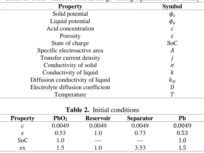
Table 1. Field variables used in the governing equations of the battery
Property Symbol
Solid potential 𝜙𝑠
Liquid potential 𝜙𝑒
Acid concentration 𝑐
Porosity 𝜀
State of charge SoC
Specific electroactive area 𝐴
Transfer current density 𝑗
Conductivity of solid 𝜎
Conductivity of liquid 𝑘
Diffusion conductivity of liquid 𝑘𝐷
Electrolyte diffusion coefficient 𝐷
Temperature 𝑇
Table 2. Initial conditions
Property PbO2 Reservoir Separator Pb
𝑐 0.0049 0.0049 0.0049 0.0049
𝜀 0.53 1.0 0.73 0.53
SoC 1.0 --- --- 1.0
ex 1.5 1.0 3.53 1.5
The equations are discretized using the finite volume method. At each time step, a value is guessed for V and then the discretized form of Eqs. 3 and 4 are solved using the Newton iteration technique. The guessed value of V is updated by the Secant method until the applied current density converges to the desired value and then the solution marches to the next time step using Eqs. 5-7. The time-marching continues until V drops below a cut-off voltage. Here, the cut-off voltage is 1.5 V
Results and Discussion
All the field variables (Table 1) are defined as array objects. Also, most of the relations are implemented by the provided classes in the framework. For instance, the transfer current density (j) is implemented as follows:
struct TransferCurrentDensity : public MultiVarFun < TransferCurrentDensity > {
__device__ static double apply(double c, double eta, double T) {
double res =
i0*pow(c / c_ref, gamma)* (
exp(alpha_a*cu_F*eta / (cu_R*T)) - exp(-alpha_c*cu_F*eta / (cu_R*T)) );
return res; }
A non-uniform grid is used for discretizing the geometry. The grid is clustered near the interface of the different regions. Eqs. 5-7 are integrated using the forward Euler method. Also, the discretized equations of the elliptic equations for the i-th volume can be written in the following general form [8]:
(18) 𝑎𝑃𝜙𝑖 = 𝑎𝑊𝜙𝑖−1+ 𝑎𝐸𝜙𝑖+1+ 𝑆𝑢
(19) 𝑎𝑃 = 𝑎𝑊+ 𝑎𝐸 + 𝑆𝑃
𝑎𝐸 = Γe
𝑥𝑖+1− 𝑥𝑖 𝑎𝑊 = Γw
𝑥𝑖− 𝑥𝑖−1
where xi is the position of the volume center and Γ is the diffusion coefficient (𝜎eff or 𝑘eff). The
subscripts w and e indicate the left and right faces of the volume, respectively. The harmonic mean is used for approximating the diffusion coefficients (Γ) at the interface of two adjacent volumes:
(20) Γ𝑒 =
ΓiΓi+1
𝛽Γi+1− (1 − 𝛽)Γi
𝛽 = 𝑥𝑒− 𝑥𝑖 𝑥𝑖+1− 𝑥𝑖
which reduces the relation of 𝑎𝐸 into scheme (2).
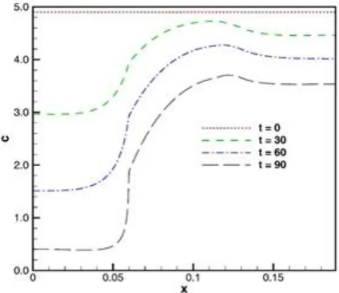
Fig. 2 shows the acid concentration at several times, using the empirical relations (Eqs. 14
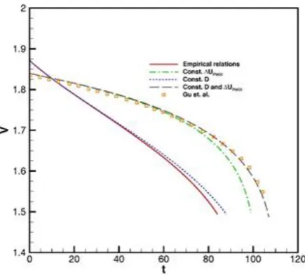
and 15). The decrease of the acid concentration in the positive electrode is faster than that of the other regions. Fig. 3 shows the cell voltage (V) during the discharge process. The simulation results corresponding to relations (13) are also validated by those of Gu et al [5]. The figure shows using a constant value for the open circuit potential (Δ𝑈PbO2) significantly affects the rate of the voltage drop. On the contrary, using a constant value for the electrolyte diffusion coefficient (D) has a slight effect on the rate of the voltage drop. Therefore, while assuming a constant value for the electrolyte diffusion coefficient is a good approximation, this is not the case for the open circuit potential.
Fig. 3. Voltage of the cell during discharge
Conclusions
In the present work, the numerical simulation of a lead-acid battery cell was carried out using a GPU framework. The framework facilitated the GPU implementation of a finite difference (or structured finite volume) numerical simulation code using C++ meta-programming techniques. It was observed the arithmetic operators, math functions, linear and nonlinear schemes were used or defined without writing a GPU kernel. The simulations indicate while assuming a constant value for the electrolyte diffusion coefficient has a negligible effect on the rate of the voltage drop, assuming a constant value for the open circuit potential significantly affects this rate.
Acknowledgments
The author would like to acknowledge the financial support of the University of Tehran and Iran's National Elites Foundation for this research under grant number 02/1/28745. The author would also like to acknowledge Javad Shahbazi for sharing his experience in solving the model equations.
Reference
[1] Veldhuizen T. Expression templates. C++ Report. 1995 Jun;7(5):26-31.
[2] Iglberger K, Hager G, Treibig J, Rüde U. Expression templates revisited: a performance analysis of current methodologies. SIAM Journal on Scientific Computing. 2012 Mar 8;34(2):C42-69. [3] Härdtlein J, Linke A, Pflaum C. Fast expression templates. In International Conference on
Computational Science 2005 May 22 (pp. 1055-1063). Springer, Berlin, Heidelberg.
[4] Esfahanian V, Ansari AB, Torabi F. Simulation of lead-acid battery using model order reduction. Journal of Power Sources. 2015 Apr 1;279:294-305.
[5] Gu H, Nguyen TV, White RE. A mathematical model of a lead‐acid cell discharge, rest, and charge. Journal of The Electrochemical Society. 1987 Dec 1;134(12):2953-60.
[6] Gu WB, Wang CY, Liaw BY. numerical modeling of coupled electrochemical and transport processes in lead‐acid batteries. Journal of The Electrochemical Society. 1997 Jun 1;144(6):2053-61.
[7] Bode H. Lead-acid batteries. United States; 1977.
![Fig. 1. Schematic of a lead-acid battery cell, with courtesy of Ref. [4].](https://thumb-us.123doks.com/thumbv2/123dok_us/8948570.1857938/5.595.71.527.67.457/fig-schematic-lead-acid-battery-cell-courtesy-ref.webp)