International Journal of Marine, Atmospheric & Earth Sciences
Journal homepage: www.ModernScientificPress.com/Journals/IJMaes.aspx
ISSN: 2327-3356
Florida, USA Article
Basement Depth Estimates of some part of Lower Sokoto
Sedimentary Basin, North-western Nigeria, Using Spectral
Depth Analysis
*Kamba AH, S Muhammad and AG Illo
Department of Science Education, Kebbi State University of Science and Technology, Aliero
* Author to whom correspondence should be addressed; E-Mail: aliyuhassankamba@gmail.com
Article history: Received 8 October 2017, Revised 10 November 2017, Accepted 16 November 2018, Published 20 November 2018.
Abstract: Basement Depth estimate of some part of lower Sokoto basin was carried out to determine the sedimentary thickness in some parts of lower Sokoto basin. The total magnetic field values of the basin, obtained by digitizing the contour maps of the basin, which was used to produce the composite map of the area. The study Area is situated between latitudes 10.500″ N to 11. 500″ N and longitude 4.00″ E to 5.00″ E. Spectral depth analysis was carried out on each of the four aeromagnetic sheets to estimate the depth to basement. The results of the spectral studies indicate an increase in sedimentation southwards; with several depressions on the basement rock. Two prominent magnetization layers of depths varying from 0.589 km to 1.249 km and 2.506 km to 3.2 km were observed. The areas, where higher sedimentary thicknesses are observed (3.2km) was found around Konkoso in sheets No 117. It is the most probable site for prospect of hydrocarbon accumulation in the area.
Keywords: Geophysical investigation; Composite map; Sedimentary thickness; Anomalies.
1. Introduction
particular concern to geoscientists, who seek to investigate it using diverse means, some for the purpose of having knowledge, while others do it for exploration of economic resources such as minerals and hydrocarbons. With the advances in technology and the need to have a clearer picture of the Earth subsurface and its contents, the Earth scientists have deemed it necessary to utilize the properties associated with Earth’s interior. Geophysics involves the application of physical principles and quantitative physical measurements in order to study the Earth’s interior. The analysis of these measurements can reveal how the earth interior varies both vertically and laterally, the interpretation of which can reveal meaningful information on the geological structures beneath (Dobrin, 1976). By working at different scales, geophysical methods may be applied to a wide range of investigations from studies of the entire earth to exploration of a localized region of the upper crust for engineering or other purposes (Kearey et al., 2004). A wide range of geophysical methods exist for each of which there is an operative physical property to which the method is sensitive. The type of physical property to which a method responds clearly determines its range of application. For instance, magnetic method is very suitable for locating buried magnetic ore bodies because of their magnetic susceptibility. Similarly, seismic and electrical methods are suitable for locating water table, because saturated rock may be distinguished from dry rock by its higher seismic velocity and higher electrical conductivity (Kearey et al., 2004). In exploration for subsurface resources, the geophysical methods are capable of detecting and delineating local features of potential interest. Geophysical methods for detecting discontinuities, faults, joints and other basement structures, include the following: magnetic, seismic, resistivity, electrical, potential field, well logging, gravity, radiometric, thermal etc (Cordell and Grouch, 1985). Some geophysical methods such as gamma- ray spectrometry and remote sensing measure surface attributes; others, such as thermal and some electrical methods are limited to detecting relatively shallow subsurface geological features. Most economic minerals, oil, gas, and groundwater lie concealed beneath the Earth surface, thus hidden from direct view. The presence and magnitude of these resources can only be ascertained by geophysical investigations of the subsurface geologic structures in the area.
2. Materials and Methods
2.1. Data Acquisition
apart. The magnetic data collected were published in the form ½ degree aeromagnetic maps on a scale of 1:100,000. The magnetic values were plotted at 10Nt (nano Tesla) interval. The maps are numbered, and names of places and coordinates (longitude and latitudes) written for easy reference and identification. The actual magnetic values were reduced by 25,000 gammas before plotting the contour map. This implies that the value 25,000 gamma is to be added to the contour values so as to obtain the actual magnetic field at a given point. A correction based on the International Geomagnetic Reference Field, (IGRF,) and epoch date January 1, 1974 was included in all the maps. The visual interpolation method that is the method of digitizing on Grid Layout was used to obtain the data from field intensity aeromagnetic maps covering the study area. The data from each digitized map is recorded in a 19 by 19 coding sheet which contains the longitude, latitude and the name of the town flown and the sheets number. The unified composite dataset for the study area was produced after removing the edge effect. Oasis montaj was used to import the dataset. The dataset consists of three columns (longitude, latitude and magnetic values). The composite map was produced using Oasis Montaj. Version 7.2.
2.2. Regional-residual Separation
Magnetic data observed in geophysical surveys comprises of the sum of all magnetic fields produced by all underground sources. The composite map produced using such data, therefore contains two important disturbances, which are different in order of sizes and generally super-imposed. The large features generally show up as trends, which continue smoothly over a considerable distance. These trends are known as regional trends. Super-imposed on the regional field, but frequently camouflaged by these, is the smaller, local disturbances which are secondary in size but primary in importance. These are the residual anomalies. They may provide direct evidence of the existence of the reservoir type structures or mineral ore bodies.
2.3. Production of Regional and Residual Maps
The residual magnetic field of the study area was produced by subtracting the regional field from the total magnetic field using the Polynomial fitting method. The computer program Aerosupermap was used to generate the coordinates of the total intensity field data values. This super data file, for all the magnetic values was used for production of composite aeromagnetic map of the study area using Oasis Montaj software version 7.1 A program was used to derive the residual magnetic values by subtracting values of regional field from the total magnetic field values to produce the residual magnetic map and the regional maps.
Determination of depths to buried magnetic rocks is among the principal applications of an aeromagnetic data. The depths are commonly computed from measurement made on the widths and slopes of an individual anomaly of the aeromagnetic profiles. The statistical approach has been found to yield good estimates of mean depth to basement underlying a sedimentary basin (Hahn et al., 1976, Udensi, 2001). Spector (1968) and Spector and Grant (1970) developed a depth determination method which matches two dimensional power spectral calculated from gridded total magnetic intensity field data with corresponding spectral obtained from a theoretical model. For the purpose of analyzing aeromagnetic data, the ground is assumed to consist of a number of independent ensembles of rectangular, vertical sided parallelepiped, and each is ensemble characterized by a joint frequency distribution for the depth (h) and length (b) and depth extent (t). In this work, the characteristics of the residual magnetic field are studied using statistical spectral methods. This is done by first transforming the data from space to the frequency domain and then analyzing their frequency characteristics. In the general case, the radial spectrum may be conveniently approximated by straight line segments, the slopes of which relate to depths of the possible layers, (Spector and Grant, 1970, and Hahn et al., 1976). The residual total magnetic field intensity values are used to obtain the two dimensional Fourier Transform, from which the spectrum is to be extracted from the residual values T (x, y) consisting of M rows and N columns in X – Y. The two dimensional Fourier transforms is obtained as given in equation (2.1) above. The evaluation is done using an algorithm that is a two dimensional extension of the fast Fourier transform (Oppenheim and Schafer, 1975). Next, the frequency intervals are subdivided into sub-intervals, which lie within one unit of frequency range. The average spectrum of the partial values together constitutes the redial spectrum of the anomalous field (Hahn et al., 1976, Kangkolo, 1996 and Udensi, 2001). The logarithm of the energy values versus frequency on a linear scale was plotted and the linear segments located; the use of Discrete Fourier Transform introduced the problem of aliasing and the truncation effect (or Gibbs phenomenon). Aliasing was reduced by the digitizing interval used in the study. Three or two linear segments could be seen from the graphs. The first points on the frequency scale was ignored because the low frequency components in the energy spectrum are generated from the deepest layers whose locations are most likely in errors. Each linear segment groups points due to anomalies caused by bodies occurring within a particular depth. If the z is the mean depth of the layer, the depth factor for this ensemble of anomalies is exp (-2zk). Thus the logarithmic plot of the radial spectrum would give a straight line whose slope is -2z. The mean depth of the burial ensemble is thus given as
2
m
Z
Where (m) is the slope of the best fitting straight line Equation 2.1 can be applied directly if the frequency unit is in radian per kilometre. If however, the frequency unit is in circle per kilometre, the corresponding relationship can be expressed as
4
m Z
2.2
3. Results and Discussion
3.1. Total Magnetic Intensity Map
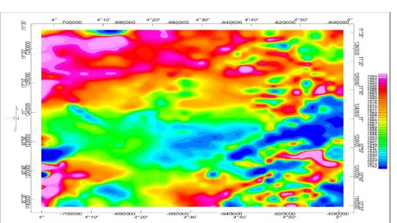
The total magnetic intensity map ﴾TMI﴿ of the study area in lower Sokoto sedimentary basin produced from this study using Oasis Montaj version 7.1 is as shown in (Figure 3.1). The TMI map of lower Sokoto sedimentary basin can be divided into three main sections, though minor depressions exist scattered all over area. The northern part of some area in lower Sokoto basin is characterized by High magnetic intensity values ranges from 7883 to 7900. Whereas the southern part is dominated by low magnetic intensity values ranges from 7792 to 7860. The two sections are separated by a zone characterized by medium magnetic intensity values area depicted by yellow-orange colour. These high magnetic intensity values, which dominate the northern part in some area of the study area in lower Sokoto Sedimentary basin, are caused probably by near surface igneous rocks of high values of magnetic susceptibilities. The low amplitudes are most likely due to sedimentary rocks and other non-magnetic sources. In general, high non-magnetic values arise from igneous and crystalline basement rocks. Whereas low magnetic values are usually from sedimentary rocks or altered basement rocks. The sedimentary thickness of some part of the study area in general, appears to increases from south to north.
Figure 3.1: Total Magnetic Intensity Map of the Study Area.
3.2. Regional Magnetic Intensity Map
8160 nano Tesla and the values decreases from south to north indicating there is a fill of sediments more in the southern part of the area than in the northern part of the study area. The result of regional indicates deeper sedimentation in the south than in the northern part of the study area.
Figure 3.2: Map of the Study Area
3.3. Residual Magnetic Intensity Map
Figure 3.3 is the residual magnetic intensity map of the study area. The residual map is characterized with positive and negative magnetic susceptibility values. The pink and red colour represents the high positive values while the blue colour represents high negative values. The pale-green and yellow colour represent the lower negative and lower positive magnetic values respectively. The magnetic intensity values ranges from -10 nano Tesla to 40 nano Tesla. Negative magnetic intensity values are more predominant in the southeast section of the study area while the northwest has more of positive magnetic intensity values. Northeast –Southwest trends are observed in the north central part of the TMI map. The blue color in the southeast indicating the area of higher sedimentation around sheet 117 (konkoso) in the study area with the prospect of hydrocarbon accumulation.
3.4. Spectral Depth Analysis
The results of the spectral analysis of the nine sections carried out in the survey area are shown in Table 1.
Table 1: Estimated depth to the shallow (depth1) magnetic sources and deep (depth2) magnetic sources
in kilometers.
Section Sheet Name
Longitude Latitude Z1(km) Z2(km)
A Konkoso 4.25 10.75 0.922 2.705
B Yelwa 4.75 10.75 0.773 2.601
C Kaoje 4.25 11.25 0.843 2.673
D Shanga 4.75 11.25 0.589 2.506
E Konkoso/Yelwa 4.50 10.75 1.169 2.840
F Kaoje/Shanga 4.50 11.25 1.249 3.111
G Konkoso/Kaoje 4.25 11.00 1.058 3.174
H Yelwa/Shanga 4.75 11.00 0.827 2.951 I Konkoso, Yelwa 4.50 11.00 1.010 2.824
Kaoje, Shanga
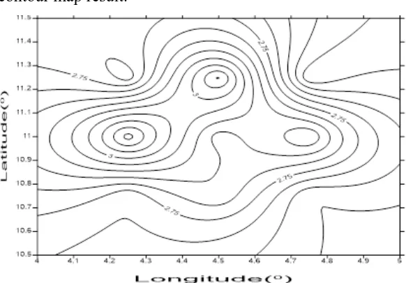
3.5. Contour Map
The contour Map and surface plot for second layer depth of the study area as shown in figures 4 and 5. The contour map of the second layer depth (H2) shows that the basement depth is deeper in the
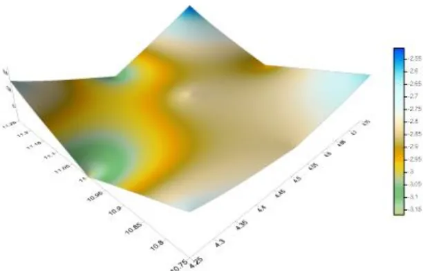
southeastern part around sheet number 117 area of konkoso. 3D surface plot shows similar thing with contour map result.
Figure 5: Surface plot map of the second layer depth
4. Conclusions
The conclusion drawn from this work, based on the results of spectral depth analysis, identified on the Total Magnetic Intensity (TMI) of some part of lower Sokoto sedimentary Basin are as follow From this study, results obtained from the spectral depth analysis carried out sheet by sheet identified areas depth average of Kaoje (2.506km), Konkoso (3.2km), Shanga (0.589km), Yelwa (1.249km) having relatively higher sedimentation.
5. Recommendations
Several depressions or variations in thickness have been observed in some parts of the lower Sokoto Basin, particularly around Konkoso (3.2km) Sheet 117 areas, these deeper sections of the study area sedimentary basin identified in this study, might be probable potential site for hydrocarbon deposits and is therefore recommended to be subjected to further investigation using other geophysical method such as seismic. Exploration of the Nigerian inland basins is worth given a push. Hydrocarbons if discovered and harnessed will increase the country’s reserve and boost productivity. All these will have economic and strategic benefits for the country.
Reference
Dobrin, M.B. (1976), Introduction to Geophysical Prospecting. Mc-Graw Hill Books Co (3rd Ed.) N.Y. Pp. 630
Hahn, A., Kind, E. and Mishra, D.C. (1976) Depth Estimate of Magnetic Sources by means of Fourier amplitude Spectra, Geophy prospecting, 24:287-308.
Huntings Geology and Geophysical ltd (1976). Airbone Magnetometer Survey Contour of Total intensity Map of Nigeria. Airbone Geophysical Series.
Kangkolo, R. (1996). A Detailed Interpretation of the Aeromagnetic field over the Manfe Basin of Nigeria and Cameroon. Unpublished Ph.D. thesis, Ahmadu Bello University, Zaria, Nigeria. Kearey P, Brooks M, Hill I(2004). An Introduction to Geophysical Exploration. Third Edition,
Blackwell Pub. N.Y. Pp. 630
Nigerian Geology Survey Agency, (1976), Geology Map of Nigeria. Scale1:2, 00 000. Geology Survey of Nigeria, Kaduna, Nigeria [7].
Oppenheim, A.V and Schafer R.W.; Digital signal processing practice. Hall International Inc. New Jersey. (1975): 1227-1296.
Spector, A. (1968).Spectral Analysis of Aeromagnetic Data: Unpublished Ph.D. Thesis, University of Toronto, Canada.
Spector, A. and Grant, F.S. (1970).Statistical Models for Interpreting Aeromagnetic Data. Geophysics,
35: 293-302.
Udensi, E. E., and Osazuwa, I. B. (2002). Two and half dimensional modeling of the major structures underlying the Nupe Basin, Nigeria using aeromagnetic data. Nigerian Journal of Physics, 14:
55-61.