An open access repository of
Middlesex University research
http://eprints.mdx.ac.uk
Zhang, Xiaoge, Adamatzky, Andrew, Chan, Felix T. S., Deng, Yong, Yang, Hai, Yang, Xin-She
ORCID: https://orcid.org/0000-0001-8231-5556, Tsompanas, Michail-Antisthenis I., Sirakoulis,
Georgios Ch. and Mahadevan, Sankaran (2015) A biologically inspired network design model.
Scientific Reports, 5 . ISSN 2045-2322
Published version (with publisher’s formatting)
This version is available at:
http://eprints.mdx.ac.uk/17011/
Copyright:
Middlesex University Research Repository makes the University’s research available electronically.
Copyright and moral rights to this work are retained by the author and/or other copyright owners
unless otherwise stated. The work is supplied on the understanding that any use for commercial gain
is strictly forbidden. A copy may be downloaded for personal, non-commercial, research or study
without prior permission and without charge.
Works, including theses and research projects, may not be reproduced in any format or medium, or
extensive quotations taken from them, or their content changed in any way, without first obtaining
permission in writing from the copyright holder(s). They may not be sold or exploited commercially in
any format or medium without the prior written permission of the copyright holder(s).
Full bibliographic details must be given when referring to, or quoting from full items including the
author’s name, the title of the work, publication details where relevant (place, publisher, date),
pag-ination, and for theses or dissertations the awarding institution, the degree type awarded, and the
date of the award.
If you believe that any material held in the repository infringes copyright law, please contact the
Repository Team at Middlesex University via the following email address:
[email protected]
The item will be removed from the repository while any claim is being investigated.
Design Model
Xiaoge Zhang1,4, Andrew Adamatzky2, Felix T.S. Chan3, Yong Deng1,4, Hai Yang5,
Xin-She Yang6, Michail-Antisthenis I. Tsompanas7, Georgios Ch. Sirakoulis7 &
Sankaran Mahadevan4
A network design problem is to select a subset of links in a transport network that satisfy passengers or cargo transportation demands while minimizing the overall costs of the transportation. We propose a mathematical model of the foraging behaviour of slime mould P. polycephalum to solve the network design problem and construct optimal transport networks. In our algorithm, a traffic flow between any two cities is estimated using a gravity model. The flow is imitated by the model of the slime mould. The algorithm model converges to a steady state, which represents a solution of the problem. We validate our approach on examples of major transport networks in Mexico and China. By comparing networks developed in our approach with the man-made highways, networks developed by the slime mould, and a cellular automata model inspired by slime mould, we demonstrate the flexibility and efficiency of our approach.
Transport networks are vital infrastructure of human society. Many networks are overloaded and often choked with traffic. Governments in most countries aim to ease congestion by imposing pollution
charges1,2, tradable travel credits for congestion management3, parking permits distribution and
trad-ing4. Such policies reduce the congestion to some extent, but they also lead to additional problems. For
example, in the policy of tradable travel credits for congestion management, it might be complicated to make a decision on how to allocate the limited tradable travel credits to users, how many tradable travel
credits should be provided, etc5–7. One of the most promising solutions to this problem would be to
design an efficient transit network for a transportation system. The efficient transit network is capable of
maximizing throughout capacity and minimizing the overall costs8–14.
The network design problem (NDP) is one of the most challenging transport problems. The problem
is defined as follows. Given a weighted graph G, we want to select such a subgraph in G that it satisfies
the given point-to-point demand on a transportation and minimizes the overall costs of the transporta-tion. In the past decades, various approaches have been presented to address this issue. The solutions can
be divided into two categories: exact solutions15–17 and heuristic solutions18–21. Exact solution methods
can deal with NDP in a rigorous manner. However, they are inefficient when dealing with large-scale
real-world networks18,22,23. Heuristic approaches, emerged in the past decades24,25, provide approximate
yet efficient solutions. The heuristic approaches can tackle a real-world problems with a large number of
design variables26,27 and therefore these approaches are more popular than exact solutions20,28–31.
When we design a transportation network we should, ideally, make it fault tolerant, capable to cope with traffic accidents, terrorist attack, and emergency road maintenance. Fault tolerance and high per-formance attract higher building and maintenance costs. How to make a tradeoff between the overall
1School of Computer and Information Science, Southwest University, Chongqing 400715, China. 2Unconventional Computing Center, University of the West of England, Bristol BS16 1QY, UK. 3Department of Industrial and Systems Engineering, The Hong Kong Polytechnic University, Hung Hum, Kowloon, Hong Kong. 4School of Engineering, Vanderbilt University, Nashiville, 37235, USA. 5Department of Civil and Environmental Engineering, The Hong Kong University of Science and Technology, Clear Water Bay, Kowloon, Hong Kong. 6School of Science and Technology, Middlesex University, London NW4 4BT, UK. 7Department of Electrical and Computer Engineering, Democritus University of Thrace, Xanthi 67100, Greece. Correspondence and requests for materials should be addressed to Y.D. (email: [email protected]) or S.M. (email: [email protected])
cost, the fault tolerance, and the performance is the problem worthwhile to investigate32–34. During their
evolution living creatures optimised their transportation networks over million of years: vascular systems
of plants and animals35,36, foraging patterns of social insects37,38 migration trails by birds and animals,
hunting routes of predators. It is therefore often very fruitful to apply natural solutions in designs of
human-made artifacts39.
There is a unique creature which exhibits properties of internal and external living transport systems.
This is a acellular slime mould Physarum polycephalum. Plasmodium is a vegetative stage of acellular
slime mould P. polycephalum, a syncytium, a single cell with many nuclei, which feeds on microscopic
particles40. When foraging for its food the plasmodium propagates towards sources of food particles,
surrounds them, secretes enzymes and digests the food. Typically, the plasmodium forms a congregation of protoplasm covering the food source. When several sources of nutrients are scattered in the plasmodi-um’s range, the plasmodium forms a network of protoplasmic tubes connecting the masses of protoplasm at the food sources.
During its foraging behaviour the plasmodium spans scattered sources of nutrients with a network of protoplasmic tubes. The protoplasmic network is optimized to cover all sources of food and to provide a robust and speedy transportation of nutrients and metabolites in the plasmodium body. The plasmo-dium’s foraging behaviour can be interpreted as a computation, where data are represented by spatial configurations of attractants and repellents, and results of the computation are protoplasmic network
formed by the plasmodium on the data sets41–43. The problems solved by plasmodium of P.
polycepha-lum include the shortest path41,42, connecting different arrays of food sources in an efficient manner44,
implementation of storage modification machines45, Voronoi diagram46, Delaunay triangulation43, logical
computing47, and process algebra48, see overview in43.
A mathematical model of Physarum morphological behavior was proposed in49. Bonifaci et al.50
demonstrated that Physarum converges to a shortest path in the network regardless of the initial
struc-ture of the network or of the initial mass distribution. In the present paper, we explore Physarum to solve
an NDP in terms of costs, efficiency and robustness. We employ the gravity model51 to estimate the traffic
flow between a pair of cities. Based on a specific travel demand, we employ Physarum to simulate the
transport flow between the cities. Then we allow the slime mould to colonise all cities, develop its proto-plasmic network and settle down in some stable sate. The stable state represents a solution of the NDP.
Results
We will evaluate the networks using measures of cost, efficiency, and robustness. In Physaurm algorithm,
a threshold value δ as shown in the supplementary material is required to stop the execution of this
pro-gram. If the threshold value δ is too small, it will take the Physarum algorithm a lot of time to converge
to a solution. If δ is too large, the results will not reflect the features of the formulated networks. Here,
we adopt a comprising strategy between the execution time of the algorithm and the characteristics of
the formulated networks. The threshold value δ is set to be 0.01.
A cost (TL) is the sum of the length of all the edges existing in each network while the length is a representative of geographical distance. We have normalized the cost TL to the total length of the Minimum Spanning Tree (MST) for the corresponding networks. Efficiency (MD) is the transportation performance of each network, which is measured as the sum of minimum distance (MD) between all
pairs of nodes. The efficiency MD is also normalized to the sum MDMST of minimum distances between
all pairs of nodes in the Minimum Spanning Tree. Finally, the fault tolerance, or robustness, of a network is measured as the probability of the network to become disconnected when a single link is removed. Here, the disconnection is defined as follows: for any pair of nodes, if there is no feasible path between them, we can say the network is disconnected. For example, in MST, the removal of any link will lead to the disconnection of the network.
Application to Mexican Highways Network. To compare our algorithm with the real slime mould,
we have used the results from our previous experimental laboratory studies52. We have selected 19 most
populated urban areas shown in Fig. 1(a). The general data on these cities are described in Table 1. Figure 1(b) shows the minimum spanning tree (MST) of Mexico highways.
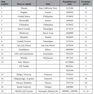
According to Eq. (8) and the data shown in Table 1, we can construct the basic traffic flow among any two cities. For the row with more than one economic power shown in Table 1, we can regard it as a single row by summing these economic powers, then the corresponding traffic flow can be determined.
Specifically speaking, for Row 14, the economic power will be 2 + 1 + 7 = 10. According to Eq. (8), we
can figure out the traffic flows from this city to the other cities.
The final step is to construct the network according to the conductivity value α associated with each
edge. α is just used to filter out the edges with conductivity less than α. α's values are determined as
fol-lows. When the Physarum algorithm is over, we will make full use of this parameter to build the networks
with different topologies. Every time, these three parameters (Cost, Performance, and Efficiency) change,
α will be recorded. We keep recording α's values until the network becomes disconnected. Generally
speaking, α's values can reflect the changing trend of these formulated networks. With the increase of
α, the less important edges will gradually fade out, which will affect the performance of the formulated
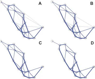
network further. In this paper, we set the starting value for α is 0.01. For example, Fig. 2 shows four
Let us now compare the transport performance, fault tolerance, and efficiency of each network. The
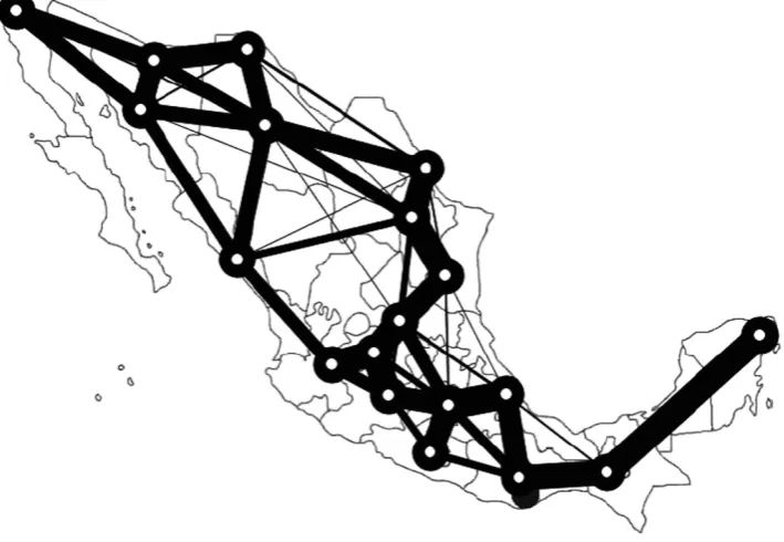
real Mexico highways and the network developed by Physarum are shown in Fig. 3. ue to the reason of
the copyright, we cannot show the structure of the real Mexico highways here. But it can be obtained from Ref. 52, which is Fig. 7(a) in Ref. 52. We also compare our results with a cellular automata model,
inspired by slime mould, proposed by Tsompanas et al.53. The cellular automata model employs an
attractant diffusion equation to describe the foraging behavior of the plasmodium and to calculate the propagation of chemoattractants produced by the nutrient sources. The diffusion of chemoattractants is
uniform, while the growth of the slime mould is affected by the concentration of chemoattractants53,54.
Note here that the parameters of the model are the same as used in54. Moreover, the input data of the
model is only the configuration of the cities in the country and its borders. No economical or population factors are taken into consideration.
Figure 1. Basis of experiments with Mexico. (a) Configuration of sources of food representing major urban areas. (b) Minimum spanning tree. The maps are generated using the locations of these cities and the boundaries of Mexico. Maps created by AA.
Map
number Town or capital State Population per state Economic power
1 Tijuana Baja California Nore 3122400 8 2 Nogales Sonora 2499263 12 3 Ciudad Juárez Chihuahua 3376052 5 4 Hermosillo Sonora 2499263 12 5 Chihuahua Chihuahua 3376052 5 6 Nuevo Laredo Tamaulipas 3174134 11 7 Monterrey Nuevo Leon 4420909 3 8 Mazatlán Sinaloa 2650499 15 9 Ciudad Victoria Tamaulipas 3174134 11 10 San Luis Potosí San Luis Potosí 2479450 14 11 Guadalajara Jalisco 6989304 4 12 Léon and Guanajuato Guanajuato 5033276 9 13 Morelia Michoacan 3971225 22 14 Edo. México, * 14739060, 2 DF, Puebla 8839361, 1 5624104 7 15 Xalapa, Veracruz Veracruz 7270413 6 16 Chilpancingo, Acapulco Guerrero 3143292 18 17 Oaxaca, Huatulco Oaxaca 3551710 20 18 Tuxtla Gutiérrez Chiapas 4483866 17 19 Merida and Cancún Yucata¡än, Qintana Ro 1909965, 1290300 21, 19
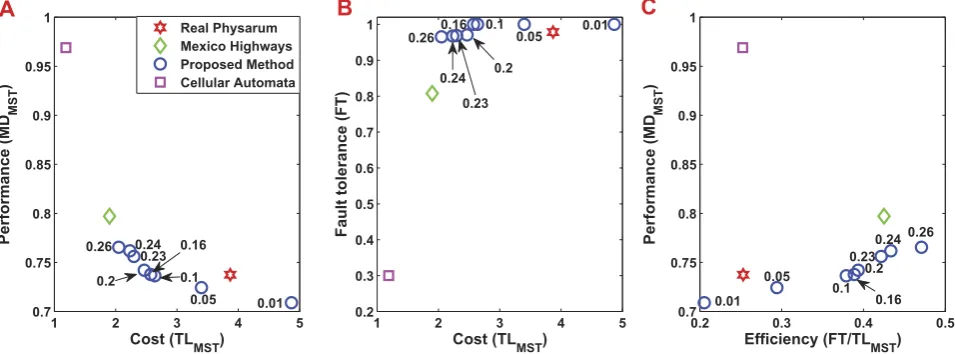
Figure 4(a) shows the Mexico highway networks built by Tsompanas’s model. The numbers near blue
circles denote the α's value associated with each formulated network. In terms of the transportation
performance, the cost of Mexican highways built by the cellular automata model is least among all the alternative networks, which is greater than the MST by a factor of 1.2. Regarding the network perfor-mance, the lower its value is, the better the performance is. However, for the network build by the cellular automata model, its transportation performance is about 0.97, which is the worst in all the networks.
For the network built by real Physarum, it can be seen that it has a factor of 3.8 when compared with
the MST. As for the network formulated by the Physarum algorithm, when α’s value ranges from 0.01 to
0.26, the transportation performance fluctuates gradually. Among them, the networks have less cost but
high transportation performance when α ranges from 0.05 to 0.26. This demonstrates that the proposed
methods are flexible. In a real-world environment, we can determine the topology of the network and
the value αaccording to the specific budget. It can be noted that when α changes from 0.05 to 0.26, the
Physarum algorithm can build networks with higher performance but lower cost when compared with
other networks. In summary, the Physarum algorithm can achieve better and flexible results with
mar-ginally lower costs.
Our Physarum algorithm also outperforms other methods in terms of fault tolerance (FT). As can be seen in Fig. 5(B), the network generated by the cellular automate model has the lowest fault tolerance about 0.3, which means about 70% of faults in this network will lead to the disconnection of any part.
However, both the network constructed by real Physarum and the Physarum algorithm have high fault
tolerance. When α is 0.01, 0.05, 0.1, 0.16, the formulated networks show the best fault tolerance, which
Figure 2. Comparison of the networks constructed by the Physarum when α has different values.
is equal to the maximum tolerance to a random failure of a single link. With the increase of α, fault
tol-erance of a network decreases gradually. As for the network grown by real Physarum, its fault tolerance
is still higher than Mexican highways, which is about 0.9787.
The trade-off between the cost and fault tolerance is measured by FT/TLMST. Mexican highways have
a high efficiency, which is about 0.42. For the real Physarum, it has a factor of 0.25. As for the networks
formulated by the Physarum algorithm, the efficiency factor becomes the highest when α is 0.26. When α
has different values (in other words, when the cost is different), the Physarum takes different measures to
adapt to these environments spontaneously. For the cellular automate-based network, the corresponding value is 0.25, which is the third lowest value for the efficiency indicator among all the alternative models.
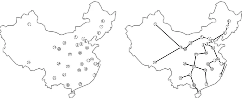
Application to China Motorways Network. In China motorways network, we choose 31 most
pop-ulated major urban areas approximately corresponding to distribution of population densities by 201055
and they are shown in Fig. 6(a). Figure. 6(b) shows the minimum spanning tree of China motorways network. Table 2 displays the population and economic power of each city.
Similarly, we can develop the networks by filtering out the edges with conductivity less than α.
Figure 7 shows us the networks for α is 0.02, 0.05, 0.07, and 0.09, respectively. As can be seen in Fig. 7,
with the increase of α, some unimportant edges gradually disappear while the critical links are retained.
The thickness of every edge reflects the actual size of the traffic flow between different cities. It can be seen that most of the edges with bigger traffic flow are mainly distributed in the central and southeastern China.
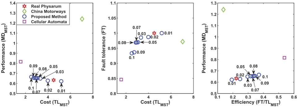
Figure 8 shows the slime mould approximation of transport network in China and the real motorways graph, respectively. Let us compare the transport performance, fault tolerance, and the efficiency of each network. The motorway network shown in Fig. 9(A) has highest cost and lowest performance. China motorways cost is bigger than MST by a factor of 7. The minimum distance between all pairs of nodes in the motorway network is higher than MST by about 25% percent. Both the networks developed by
real Physarum and the proposed Physarum algorithm have less cost. When α is 0.01, Physarum algorithm
has more cost when compared with the network built by real Physarum but its performance is better
than the performance of the real Physarum. In addition, with the increase of α, the performance of every
network constructed by Physarum algorithm decreases gradually while its cost reduces by a larger size.
For the cellular automata based network, the constructed network has lowest cost but the performance is the second worst in all the alternatives.
As for the fault tolerance of each network, from Fig. 9, it can be noted that although the cost of China motorways is very high, its fault tolerance is still lower when compared with the network formulated by
real Physarum and the network built by Physarum algorithm when α= 0.01. With the change of α, the
fault tolerance of the networks built by Physarum algorithm changes a little when compared with the
change of its cost. While the network formulated by the cellular automate model has the lowest cost, its
Figure 3. Mexico transport networks developed by the slime mould52. The maps are generated using the
fault tolerance is also lowest among all alternatives. The fault tolerance requires a presence of redundant links in the network therefore it increases the cost of the network.
Finally, let us focus on the efficiency of every network. For α= 0.1 the network has the highest
effi-ciency. When α changes, the cost’s change amplitude is greater than the fault tolerance’s. Among these
networks, China motorways has the lowest efficiency while the network formulated by real Physarum
is the third lowest. Although the network formulated by the cellular automata model has the highest efficiency, both the performance and the fault tolerance of this network is very worse. In the real-world transportation systems, we need to account for all the three parameters. From this point of view, all the
above may suggest that the networks formulated by Physarum algorithm are highly efficient. Thus, it is
useful to implement this method into real-world applications, such as the transportation network design.
Figure 4. The transportation networks developed by the Physarum-inspired cellular automata models.
(a) Mexico highways (b) China motorways. The maps are generated by the Physarum-inspired cellular automata models. Maps created by MAT and GS.
Figure 5. Transport performance, fault tolerance, and efficiency for the network developed by real
Discussion
We applied a model of foraging behaviour of slime mould Physarum polycephalum to solve a network
design problem by maximising transport capacity of the network and minimising the size and length
of the network. The Physarum algorithm solved the network design problem by developing competition
between transport routes: the links with high transportation loads increase their conductivity while less used links are removed. We demonstrated the efficiency of the proposed algorithm by comparing
net-works produced by the Physarum algorithm with networks of man-made highway network in Mexico
and motorways networks in China and protoplasmic transport networks grown by the slime mould on
a map of major urban areas of Mexico and China and a Physarum-inspired cellular automate model.
The networks were compared in terms of costs, fault tolerance and efficiency. We demonstrated that the
Physarum algorithm produces network which are superior in terms of costs, tolerance and efficiency. Further research will develop in two directions. First, we will adapt the algorithm to the design of sensor, mobile and telecommunication networks. One possible extension of the algorithms would be to incorporate traffic congestion into the network design problem or to consider the problem with traffic equilibrium constraint. Second, we will explore a possibility of implementing the algorithm on a parallel computer. The slime mould is an intrinsically parallel computer: it senses its environment via thousands of receptors distributed in its body, it makes ‘calculations’ via interactions of excitation and peristaltic waves originated from thousands of bio-chemical oscillators. Thus most algorithms inspired by the slime mould are receptive to parallelisation. Ideally we can ‘physically’ map networks optimised into a parallel processor: each elementary processor will be ‘responsible’ for a single node of the network. Figuratively speaking, nodes of the network will be interacting with each other and collectively evolving to an optimal topology of the network.
Methods
The proposed method consists of two steps. First, we analyse the traffic flows in a network based on the
gravity model. Second, the Physarum algorithm is employed to deal with the network design problem.
Network Design Problem56. A highway network can be described in terms of nodes or vertices,
connected by links. Some of the nodes represent the origins of the transportation demand while others are the destinations of the traffic flow. The network design problem (NDP) is to select links in a network
to satisfy the demands of transport capacity and minimise overall costs of transportation56.
Consider a network G(V,E), where V denotes a set of nodes, a weight function L, a budget B and a
criteria threshold value C. Is there a subgraph G′ (V,E′ ) of G with weight and criterion value F(G′ )≤C,
where F(G′ ) denotes the sum of the weights of the shortest paths in G′ between all pairs of vertices?
Physarum Polycephalum Inspired Shortest Path Finding Model. Physarum Polycephalum is a large, single-celled amoeboid organism forming a dynamic tubular network connecting the discovered food sources during foraging. The mechanism of tube formation can be described as follows. Tubes thicken in a given direction when shuttle streaming of the protoplasm persists in that direction for a certain time. There is a positive feedback between flux and tube thickness, as the conductance of the sol is greater in a thicker channel. With this mechanism in mind, a mathematical model illustrating the
shortest path finding has been constructed49.
Suppose the shape of the network formed by the Physarum is represented by a graph, in which a
plasmodial tube refers to an edge of the graph and a junction between tubes refers to a node. Two
Figure 6. Basis of experiments with China66. (a) Configuration of sources of food representing major
special nodes labeled as N1, N2 act as the starting node and ending node, respectively. The other nodes
are labeled as N3, N4, N5, N6, etc. The edge between node Ni and Nj is expressed as Mij. The parameter
Qij denotes the flux through tube Mij from node Ni to Nj. Assume the flow along the tube be an
approx-imately Poiseuille flow, then flux Qij can be expressed as:
(
)
= −
( )
Q D
L p p 1
ij ij
ij i j
where pi is a pressure at a node Ni, Dij is a conductivity of a tube Mij, and Lij is its length.
By considering that the inflow and outflow must be balanced, we have:
∑
Qij= ( ≠ , )0 j 1 2 ( )2For the source node N1 and the sink node N2 the following two equations hold
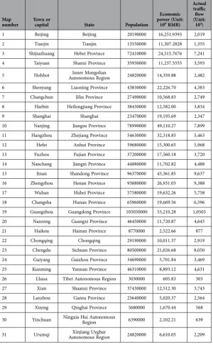
Map
number Town or capital State Population
Economic power (Unit:
109RMB)
Actual traffic flow (Unit:
104)
1 Beijing Beijing 20190000 16,251.9393 2,019 2 Tianjin Tianjin 13550000 11,307.2828 1,355 3 Shijiazhuang Hebei Province 72410000 24,515.7676 7,241 4 Taiyuan Shanxi Province 35930000 11,237.5555 3,593 5 Hohhot Autonomous RegionInner Mongolian 24820000 14,359.88 2,482 6 Shenyang Liaoning Province 43830000 22,226.70 4,383 7 Changchun Jilin Province 27490000 10,568.83 2,749 8 Harbin Heilongjiang Province 38430000 12,582.00 3,834 9 Shanghai Shanghai 23470000 19,195.69 2,347 10 Nanjing Jiangsu Province 78990000 49,110.27 7,899 11 Hangzhou Zhejiang Province 54630000 32,318.85 5,463 12 Hefei Anhui Province 59680000 15,300.65 5,968 13 Fuzhou Fujian Province 37200000 17,560.18 3,720 14 Nanchang Jiangxi Province 44880000 11,702.82 4,488 15 Jinan Shandong Province 96370000 45,361.85 9,637 16 Zhengzhou Henan Province 93880000 26,931.03 9,388 17 Wuhan Hubei Province 57580000 19,632.26 5,758 18 Changsha Hunan Province 65960000 19,669.56 6,596 19 Guangzhou Guangdong Province 105050000 53,210.28 1,0505 20 Nanning Guangxi Province 46450000 11,720.87 4,645 21 Haikou Hainan Province 8770000 2,522.66 877 22 Chongqing Chongqing 29190000 10,011.37 2,919 23 Chengdu Sichuan Province 80500000 21,026.68 8,050 24 Guiyang Guizhou Province 34690000 5,701.84 3,469 25 Kunming Yunnan Province 46310000 8,893.12 4,631 26 Lhasa Tibet Autonomous Region 3030000 605.83 303 27 Xian Shaanxi Province 37430000 12,512.30 3,743 28 Lanzhou Gansu Province 25640000 5,020.37 2,564 29 Xining Qinghai Province 5680000 1,670.44 568 30 Yinchuan Ningxia Hui Autonomous Region 6390000 2,102.21 639
31 Urumqi Autonomous RegionXinjiang Uyghur 24820000 6,610.05 2,209
∑
+ =( )
Q I 0
3
i i1 0
∑
− =( )
Q I 0
4
i i2 0
where I0 is the flux flowing from the source node and I0 is a constant value here.
Figure 7. Comparison of the networks constructed by the Physarum for different values of α . (A) The network constructed by Physarum when the edges with conductivity α less than 0.02 are filtered out. (B) The network with edges with α less than 0.05 are eliminated. (C) The constructed network when α is 0.07. (D) The developed network when α is 0.09.
In order to describe such an adaptation of tubular thickness we assume that the conductivity Dij
changes over time according to the flux Qij. An evolution of Dij(t) can be described by the following
equation:
( )
γ= − ( )
d
dtDij f Qij Dij 5
where γ is a decay rate of the tube. The equation implies that a conductivity becomes nil if there no flux
along the edge. The conductivity increases with the flux. The f is monotonically increasing continuous
function satisfying f(0) = 0.
Then the network Poisson equation for the pressure can be obtained from the Eq. (1)-(4) as follows:
(
)
∑
− = − = = , . ( ) DL p p
I for j I for j
otherwise 1 2 0 6 i ij
ij i j
0 0
By setting p2= 0 as a basic pressure level, all pi can be determined by solving Eq. (6) and Qij can also
be obtained.
In this paper, f Q( ) = Q is used because f Q
( )
ij = Q, =γ 1, Physarum can always converge tothe shortest path regardless of whether the distribution of conductivities in the initial state is random or
biased49. With the flux calculated, the conductivity can be derived, where Eq. (7) is used instead of Eq.
(5), adopting the functional form f Q( ) = Q.
δ − = − ( ) + + D D
t Q D 7
ijn ijn
ijn 1
1
Here, D +
ijn 1 represents the conductivity on link (i,j) in the n + 1 iteration. The first part |Q| in the
above equation means the acquired energy while the second part D +
ijn 1 denotes the energy consumed by
Physarum. For details, please refer to Ref. 49.
The Gravity Model. Gravity models are trip distribution models, which have been widely used in
transportation systems for estimating the traffic flow between the origins and the destinations57–62. The
gravity model adapts the concept of the law of universal gravitation: it takes into consideration the pop-ulation of two different places, corresponding to mass in gravity, and the distance between them. The gravity model can be expressed in the following form:
Figure 9. Transport performance, fault tolerance, and efficiency for the network developed by real
=
( )
α α α
F rM M
D 8
ij i j
ij
1 2
3
where Fij represents the traffic flow starting from node i to node j; Mi and Mj denote the economic sizes
of these two places, respectively; Dij is an economic cost associated with these two positions, such as the
distance between them, G is an index and it has a constant value. Here, the traffic flow for an individual
city is meant to the sum of outward traffic flow.
In the past decades, many researchers have shown that the traffic flow is highly dependent on Gross
Domestic Product (GDP) of the associated areas. For example, Cline et al.63 demonstrated that there was
a positive relationship between GDP and freight traffic. Zhang and Guo64 found that the air traffic flow
of Beijing International Airport and its corresponding GDP was positively correlated with the correla-tion coefficient up to 0.968. From this point of view, GDP can be used to predict the actual traffic flow. Except that, GDP is a comprehensive indicator. In this indicator, it has accounted for many factors, such as population, industries, income, etc, which in turn reflects development level of a city. As a result, it is more comprehensive in comparison with population. Hence, we will use GDP to represent the economic sizes of the cities.
On the other hand, with the rapid development of transportation networks, including air traffic net-works, railways netnet-works, and highway netnet-works, the world has become smaller than before. In this case,
the factor distance is not so important as before. For example, Marimoutou et al.65 explicitly stated that
The larger the partner’s GDP, the less will be the distance effect on trade . Kwon and Jung59 revealed that
the total bus flows between cities depends on only its population size. As a result, we assume that the traffic flow depends on the square root of the product of the GDP of city A and the GDP of city B, but
has no relation with the distance between them. As a result, α1,α2 are set the same value 0.5. At the same
time, as traffic flow has no relation with the distance between these cities, as a result, α3 is 0.
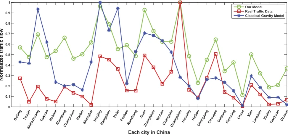
In order to confirm our assumption, we have compared our model with real traffic data and the classical gravity model for the traffic flow of China in 2011. In classical gravity model, they predict the traffic flow as the square root of the product of the population of city A and city B over the square of the distance between them. Based on the data shown in Table 2, by normalizing the traffic flow, we display the traffic flow prediction results between these models in Fig. 10. As can be noted that, the proportions traffic flow trends uncovered in our model and observed in the real traffic data are similar. We can change
the prediction results proportionally by adjusting the value of r existing in Eq. (8). However, for the
clas-sical gravity model, there are obvious differences between the prediction results and the real traffic data. For example, in the classical gravity model, Nanjing has the biggest traffic flow while in real traffic data, Guangzhou has the highest traffic volume. This in turn demonstrates the correctness of our assumption and the efficiency of our method.
Physarum Model for Network Design Problem. Consider a network G(V,E), where V denotes a set of nodes, E represents a set of arcs, Lij represents the length of edge (i,j). Assume F is a set of traffic
flow in the network G and Fij denotes the traffic flow from the origin i to the destination j. Ft represents
a number of O-D pairs (Here, the O-D pairs denotes the table of origin-destination demand) in F. Here,
Eq. (6) is expressed in the following form:
(
)
∑
− = − = , = , . ( ) DL p p
F for j s
F for j e
otherwise
0 9
i ij
ij i j
ij ij
Next, nodes i and j are starting and ending node in the Physarum model, respectively. The Physarum
algorithm runs only for one iteration when i= j.
Each link in the network is filled with some flux and their conductivity changes correspondingly. As assume the links obtain some energy from the flux whilst some energy will be also consumed. We
employ Physarum to simulate the traffic flow onthe link Fik (i,k) ∈ E, the procedure is similar with that
of traffic flow Fij. Energy in the network is limited. Therefore, all the links compete with each other for
traffic. Unused links gradually fade and disappear.
At this step, we record the conductivity matrix Dkij, which expresses the conductivity matrix when the
algorithm of Physarum starting from node i to node j is iterated for kth times. The conductivity matrix
of other O-D pairs in the kth iteration can be retained and they are expressed as
( = ,, , = ,, )
D ikij 1 N j 1 N . To reflect the functioneach O-D pair plays in the network, the
follow-ing Eq. (10) is constructed.
∑ ∑
= ( ) = = D D 10 k i N j N kij 1 1To achieve convergence of the Physarum algorithm, we must keep a scale of the conductivity matrix
D ranging from 0 to 1. As a result, the following normalised measure is obtained:
( , ) = ( , )
( )( = ,, , = ,, ) ( )
D i j D i j
D i N j N
max 1 1 11
k k
k
where max(Dk) expresses the largest value in the conductivity matrix Dk.
In what follows, Dk will be input as the initialised value of the conductivity matrix for the (k+ 1)th
iteration. The algorithm runs until a termination criterion is met. There could be several possible ter-mination criteria, including a maximum number of iterations achieved or stationary flux through each tube recorded. In present paper, we adopt the following termination criterion: the algorithm stops when values of conductivity matrix elements stabilize. A general flow of this method is shown in Algorithm 1.
References
1. Chen, L., & Yang, H. Managing congestion and emissions in road networks with tolls and rebates. Transp. Res. Part B:
Methodological46, 933–948 (2012).
2. Baublys, A., & Išoraitė, M. Improvement of external transport cost evaluation in the context of Lithuanias integration into the
European Union. Transport Reviews25, 245–259 (2005).
3. Yang, H., & Wang, X. Managing network mobility with tradable credits. Transp. Res. Part B: Methodological45, 580–594 (2011). 4. Zhang, X., Yang, H., & Huang, H. J. Improving travel efficiency by parking permits distribution and trading. Transp. Res. Part B:
Methodological45, 1018–1034 (2011).
5. Nie, Y. M. Transaction costs and tradable mobility credits. Transp. Res. Part B: Methodological46, 189–203 (2012).
6. Xiao, F., Qian, Z. S., & Zhang, H. M. Managing bottleneck congestion with tradable credits. Transp. Res. Part B: Methodological 56, 1–14 (2013).
7. Wang, X., & Yang H. Bisection-based trial-and-error implementation of marginal cost pricing and tradable credit scheme. Transp. Res. Part B: Methodological46, 1085–1096 (2012).
8. Berger, R. T., & Raghavan, S. Long-distance access network design. Manage. Sci.50, 309–325 (2004).
9. Balakrishnan, A., Magnanti, T. L., & Mirchandani, P. A dual-based algorithm for multi-level network design. Manage. Sci.40,
567–581 (1994).
10. D’Andreagiovanni, F., Carlo M., & Antonio S. Gub covers and power-indexed formulations for wireless network design. Manage. Sci.59, 142–156 (2013).
11. Pishvaee, M. S., Farahani, R. Z., & Dullaert, W. A memetic algorithm for bi-objective integrated forward/reverse logistics network design. Comput. Oper. Res.37, 1100–1112 (2010).
12. Crainic, T. G. Service network design in freight transportation. Eur. J. Oper. Res.122, 272–288 (2000).
13. Verter, V., & Kara, B. Y. A path-based approach for hazmat transport network design. Manage. Sci.54, 29–40 (2008). 14. Mauttone, A., & Urquhart, M. E. A route set construction algorithm for the transit network design problem. Comput. Oper. Res.
36, 2440–2449 (2009).
15. Dionne, R., & Florian, M. Exact and approximate algorithms for optimal network design. Networks9, 37–59 (1979).
16. Gabrel, V., Knippel, A., & Minoux, M. Exact solution of multicommodity network optimization problems with general step cost functions. Oper. Res. Lett.25, 15–23 (1999).
17. Davis, G. A. Exact local solution of the continuous network design problem via stochastic user equilibrium assignment. Transp. Res. Part B: Methodological28, 61–75 (1994).
18. Dressler, F., & Akan, O. B. Bio-inspired networking: from theory to practice. IEEE Commun. Mag.48, 176–183 (2010). 19. Juang, C. F. A hybrid of genetic algorithm and particle swarm optimization for recurrent network design. IEEE Trans. on Cybern.
28. Poorzahedy, H., & Rouhani, O. M. Hybrid meta-heuristic algorithms for solving network design problem. Eur. J. Oper. Res.182,
578–596 (2007).
29. Tom, V. M., & Mohan, S. Transit route network design using frequency coded genetic algorithm. J. Transp. Eng. 129, 186–195 (2003).
30. Zhang, X. et al. IFSJSP: a novel methodology for the job-shop scheduling problem based on intuitionistic fuzzy sets. Int. J. Prod. Res.51, 5100–5119 (2013).
31. Wang, C., Yu, S., Chen, W., & Sun, C. Highly efficient light-trapping structure design inspired by natural evolution. Sci. Rep.3,
doi:10.1038/srep01025, (2013).
32. Su, Z. et al. Robustness of interrelated traffic networks to cascading failures. Sci. Rep.4, doi:10.1038/srep05413, (2014). 33. Latora, V., & Marchiori, M. Efficient behavior of small-world networks. Phys. Rev. Lett. 87, 198701 (2001).
34. Bicchi, A., & Pallottino, L. On optimal cooperative conflict resolution for air traffic management systems. IEEE Trans. Intell. Transp. Syst. 1, 221–231 (2000).
35. Dickinson, M. H. et al. How animals move: an integrative view. Science288, 100–106 (2000).
36. Nakagaki, T., Yamada, H., & Ágota Tóth, A. Intelligence: Maze-solving by an amoeboid organism. Nature407, 470–470 (2000). 37. Solnon, C. Ants can solve constraint satisfaction problems. IEEE Trans. Evol. Comput.6, 347–357 (2002).
38. Detrain, C., Natan, C., Deneubourg, J. L. The influence of the physical environment on the self-organised foraging patterns of ants. Naturwissenschaften88, 171–174 (2001).
39. Krasnogor, N., Giuseppe, N., Mario, P., & David, P. Nature inspired cooperative strategies for optimization (nicso 2007), Springer, (2008)
40. Stephenson, S. L., Stempen, H., & Hall, I. Myxomycetes: a handbook of slime molds (Timber Press, Oregon, 1994).
41. Nakagaki, T., Yamada, H., & Ueda, T. Interaction between cell shape and contraction pattern in the physarum plasmodium.
Biophys. Chem.84, 195–204 (2000).
42. Nakagaki, T., Yamada, H., & Toth, A. Path finding by tube morphogenesis in an amoeboid organism. Biophys. Chem.92, 47–52 (2001).
43. Adamatzky, A. Physarum machines: computers from slime mould (World Scientific, Singapore, 2010). 44. Tero, A. et al. Rules for biologically inspired adaptive network design. Science327, 439–442 (2010).
45. Adamatzky, A. Physarum machine: implementation of a kolmogorov-uspensky machine on a biological substrate. Parallel
Processing Lett. 17, 455–467 (2007).
46. Shirakawa, T., Adamatzky, A., Gunji, Y. P., & Miyake, Y. On simultaneous construction of voronoi diagram and delaunay triangulation by physarum polycephalum. Int. J. Bifurcation Chaos19, 3109–3117 (2009).
47. Tsuda, S., Aono, M., & Gunji, Y. P. Robust and emergent physarum logical-computing. Biosystems73, 45–55 (2004). 48. Schumann, A., & Adamatzky, A. Physarum spatial logic. New Mathematics and Natural Computation7, 483–498 (2011). 49. Tero, A., Kobayashi, R., & Nakagaki, T. A mathematical model for adaptive transport network in path finding by true slime mold.
J. Theor. Biol.244, 553–564 (2007).
50. Bonifaci, V., Mehlhorn, K., & Varma, G. Physarum can compute shortest paths. J. Theor. Biol.309, 121–133 (2012).
51. Erlander, S., & Stewart, N. F. The gravity model in transportation analysis: theory and extensions, Vol. 3 (VSP, Netherlands, 1990). 52. Adamatzky, A., Martinez, G. J., Chapa-Vergara, S. V., Asomoza-Palacio, R., & Stephens, C. R. Approximating mexican highways
with slime mould. Natural Computing10, 1195–1214 (2011).
53. Tsompanas, M. A., Sirakoulis, G., & Adamatzky, A. Evolving transport networks with cellular automata models inspired by slime
mould. IEEE Trans. on Cybern. doi: 10.1109/TCYB.2014.2361731, (2014).
54. Tsompanas, M. A., Sirakoulis, G., & Adamatzky, A. Physarum in silicon: the Greek motorways study. Nat. Comput. doi: 10.1007/ s11047-014-9459-0, (2014).
55. China Population. National Bureau of Statistics of China. http://data.stats.gov.cn/datamap/index?m= fsnd, (2011) (Date of access: 20/08/2014).
56. Johnson, D. S., Lenstra, J. K., & Kan, A. H. G. The complexity of the network design problem. Networks8, 279–285 (1978). 57. Evans, S. P. A relationship between the gravity model for trip distribution and the transportation problem in linear programming.
Transp. Res. 7, 39–61 (1973).
58. Carrere, C. Revisiting the effects of regional trade agreements on trade flows with proper specification of the gravity model. Eur. Econ. Rev.50, 223–247 (2006).
59. Kwon, O., & Jung, W. S. Intercity express bus flow in korea and its network analysis. Physica A391, 4261–4265 (2012). 60. Simini, F., González, M. C., Maritan, A., & Barabási, A. L. A universal model for mobility and migration patterns. Nature484,
96–100 (2012).
61. Simini, F., Maritan, A. & Néda, Z. Human mobility in a continuum approach. Plos one8, e60069 (2013).
62. Ren, Y., Ercsey-Ravasz, M., Wang, P., González, M. C., & Toroczkai, Z. Predicting commuter flows in spatial networks using a
radiation model based on temporal ranges. Nat. Commun.5 doi:10.1038/ncomms6347, (2014).
63. Cline, R. C., Ruhl, T. A., Gosling, G. D., & Gillen, D. W. Air transportation demand forecasts in emerging market economies: a case study of the Kyrgyz Republic in the former Soviet Union. J. Air Transport Manage. 4, 11–23 (1998).
64. Zhang, Z., & Guo, S. Gray interval prediction of air traffic flow of capital airport. J. Civil Aviat. Univ. of China25, 1–4 (2007). 65. Marimoutou, V., Peguin, D., & Peguin-Feissolle, A. The” distance-varying” gravity model in international economics: is the
distance an obstacle to trade? Economics Bulletin29, 1157–1173 (2009).
66. Adamatzky, A., Yang, X. S., & Zhao, Y. X. Slime mould imitates transport networks in China. Int. J. Intell. Comput. and Cybern.
Acknowledgment
The work is partially supported Chongqing Natural Science Foundation, Grant No. CSCT, 2010BA2003, National Natural Science Foundation of China, Grant Nos. 61174022 and 71271061, National High Technology Research and Development Program of China (863 Program) (No.2013AA013801), Science and Technology Planning Project of Guangdong Province, China (2010B010600034, 2012B091100192), Business Intelligence Key Team of Guangdong University of Foreign Studies (TD1202), Doctor Funding of Southwest University Grant No. SWU110021.
Author Contributions
X.Z., A.A., F.T.S.C., S.M. designed and performed research. X.Z. wrote the paper. Y.H., M.A.T., G.S. performed the computation. X.S.Y. and Y.D. analyzed the data. All authors discussed the results and commented on the manuscript.
Additional Information
Supplementary information accompanies this paper at http://www.nature.com/srep
Competing financial interests: The authors declare no competing financial interests.
How to cite this article: Zhang, X. et al. A Biologically Inspired Network Design Model. Sci. Rep.5, 10794; doi: 10.1038/srep10794 (2015).