Graph convolutional networks:
a comprehensive review
Si Zhang
1*, Hanghang Tong
1, Jiejun Xu
2and Ross Maciejewski
3Introduction
Graphs naturally arise in many real-world applications, including social analysis [1], fraud detection [2, 3], traffic prediction [4], computer vision [5], and many more. By representing the data as graphs, the structural information can be encoded to model the relations among entities, and furnish more promising insights underlying the data. For example, in a transportation network, nodes are often the sensors and edges repre-sent the spatial proximity among sensors. In addition to the temporal information pro-vided by the sensors themselves, the graph structure modeled by the spatial correlations leads to a prominent improvement in the traffic prediction problem [4]. Moreover, by
Abstract
Graphs naturally appear in numerous application domains, ranging from social analysis, bioinformatics to computer vision. The unique capability of graphs enables capturing the structural relations among data, and thus allows to harvest more insights com-pared to analyzing data in isolation. However, it is often very challenging to solve the learning problems on graphs, because (1) many types of data are not originally struc-tured as graphs, such as images and text data, and (2) for graph-strucstruc-tured data, the underlying connectivity patterns are often complex and diverse. On the other hand, the representation learning has achieved great successes in many areas. Thereby, a potential solution is to learn the representation of graphs in a low-dimensional Euclid-ean space, such that the graph properties can be preserved. Although tremendous efforts have been made to address the graph representation learning problem, many of them still suffer from their shallow learning mechanisms. Deep learning models on graphs (e.g., graph neural networks) have recently emerged in machine learning and other related areas, and demonstrated the superior performance in various problems. In this survey, despite numerous types of graph neural networks, we conduct a com-prehensive review specifically on the emerging field of graph convolutional networks, which is one of the most prominent graph deep learning models. First, we group the existing graph convolutional network models into two categories based on the types of convolutions and highlight some graph convolutional network models in details. Then, we categorize different graph convolutional networks according to the areas of their applications. Finally, we present several open challenges in this area and discuss potential directions for future research.
Keywords: Graph convolutional networks, Graph representation learning, Deep learning, Spectral methods, Spatial methods, Aggregation mechanism
Open Access
© The Author(s) 2019. This article is distributed under the terms of the Creative Commons Attribution 4.0 International License (http://creat iveco mmons .org/licen ses/by/4.0/), which permits unrestricted use, distribution, and reproduction in any medium, provided you give appropriate credit to the original author(s) and the source, provide a link to the Creative Commons license, and indicate if changes were made.
RESEARCH
*Correspondence: [email protected]
1 University of Illinois
modeling the transactions among people as a graph, the complex transaction patterns can be mined for synthetic identity detection [3] and money laundering detection [6].
However, the complex structure of graphs [7] often hampers the capability of gain-ing the true insights underlygain-ing the graphs. Such complexity, for example, resides in the non-Euclidean nature of the graph-structured data. A potential solution to dealing with the complex patterns is to learn the graph representations in a low-dimensional Euclidean space via embedding techniques, including the traditional graph embedding methods [8–10], and the recent network embedding methods [11, 12]. Once the low-dimensional representations are learned, many graph-related problems can be easily done, such as the classic node classification and link prediction [12]. There exist many thorough reviews on both traditional graph embedding and recent network embed-ding methods. For example, Yan et al. review several well-established traditional graph embedding methods and discuss the general framework for graph dimensionality reduc-tion [13]. Hamilton et al. review the general graph representation learning methods, including node embedding and subgraph embedding [14]. Furthermore, Cui et al. dis-cuss the differences between the traditional graph embedding and the recent network embedding methods [15]. One notable difference is that the recent network embedding is more suitable for the task-specific network inference. Other existing literature reviews on network embedding include [16, 17].
Despite some successes of these embedding methods, many of them suffer from the limitations of the shallow learning mechanisms [11, 12] and might fail to discover the more complex patterns behind the graphs. Deep learning models, on the other hand, have been demonstrated their power in many applications. For example, convolution neural networks (CNNs) achieve a promising performance in many computer vision [18] and natural language processing [19] applications. One key reason of such successes is that CNN models can highly exploit the stationarity and compositionality properties of certain types of data. In particular, due to the grid-like nature of images, the convolu-tional layers in CNNs enable to take advantages of the hierarchical patterns and extract high-level features of the images to achieve a great expressive capability. The basic CNN models aim to learn a set of fixed-size trainable localized filters which scan every pixel in the images and combine the surrounding pixels. The core components include the convolutional and pooling layers that can be operated on the data with an Euclidean or grid-like structure.
domain (i.e., vertex domain) as the aggregations of node representations from the node neighborhoods. The emergence of these operations opens a door to graph convolutional networks. Generally speaking, graph convolutional network models are a type of neural network architectures that can leverage the graph structure and aggregate node informa-tion from the neighborhoods in a convoluinforma-tional fashion. Graph convoluinforma-tional networks have a great expressive power to learn the graph representations and have achieved a superior performance in a wide range of tasks and applications. Note that in the past few years, many other types of graph neural networks have been proposed, including (but are not limited to): (1) graph auto-encoder [21], (2) graph generative model [22, 23], (3) graph attention model [24, 25], and (4) graph recurrent neural networks [26, 27].
There exist several other related surveys on the topic of graph neural networks. Bron-stein et al. review the mathematical details and a number of early approaches of geo-metric deep learning for both graphs and manifolds [28]. Zhang et al. present a detailed review that covers many existing graph neural networks beyond graph convolutional networks, such as graph attention networks and gated graph neural network [29]. In addition, Wu et al. also review the studies on graph generative models and neural net-works for spatial-temporal netnet-works [30]. Besides, Lee et al. present an overview of graph neural networks with a special focus on graph attention networks [31]. However, since graph convolutional network is a very hot and fast developing research area, these existing surveys may not cover the most up-to-date models. In this survey, we focus spe-cifically on reviewing the existing literature of the graph convolutional networks and cover the recent progress. The main contributions of this survey are summarized as follows:
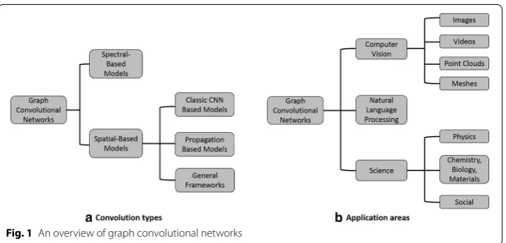
1. We introduce two taxonomies to group the existing graph convolutional network models (Fig. 1). First, we categorize graph convolutional networks into spectral-based and spatial-spectral-based models depending on the types of convolutions. Then, we introduce several graph convolutional networks according to their application domains.
2. We motivate each taxonomy by surveying and discussing the up-to-date graph con-volutional network models.
3. We discuss the challenges of the current models that need to be addressed and high-light some promising directions for the future work.
The rest of the paper is organized as follows. We start by summarizing the notations and introducing some preliminaries of graph convolutional networks in “Notations and pre-liminaries” section. Then, in “Spectral graph convolutional networks” and “Spatial graph convolutional networks” sections, we categorize the existing models into the spectral-based methods and the spatial-spectral-based methods by the types of graph filtering with some detailed examples. “Applications of graph convolutional networks” section presents the methods from a view of applications. In “Challenges and future researches” section, we discuss some challenges of the existing graph convolutional network models and pro-vide some directions for the future work. Finally, we conclude our survey in “Concluding remarks” section.
Notations and preliminaries
In this section, we present the notations and some preliminaries for the graph convolu-tional networks. In general, we use bold uppercase letters for matrices, bold lowercase letters for vectors, and lowercase letters for scalars. For matrix indexing, we use A(i,j) to
denote the entry at the intersection of the ith row and jth column. We denote the trans-pose of a matrix A as AT.
Graphs and graph signals
In this survey, we are interested in the graph convolutional network models on an undi-rected connected graph G= {V,E, A} , which consists of a set of nodes V with |V| =n ,
a set of edges E with |E| =m and the adjacency matrix A . If there is an edge between node i and node j, the entry A(i,j) denotes the weight of the edge; otherwise, A(i,j)=0 .
For unweighted graphs, we simply set A(i,j)=1 . We denote the degree matrix of A as a diagonal matrix D , where D(i,i)=nj=1A(i,j) . Then, the Laplacian matrix of A is denoted as L=D−A . The corresponding symmetrically normalized Laplacian matrix
is L˜ =I−D−1
2AD−12 , where I is an identity matrix.
A graph signal defined on the nodes is represented as a vector x∈Rn , where x(i) is the
signal value on the node i [20]. Node attributes, for instance, can be considered as the graph signals. Denote X∈Rn×d as the node attribute matrix of an attributed graph, and
then, the columns of X are the d signals of the graph.
Graph Fourier transform
It is well-known that the classic Fourier transform of an 1-D signal f is computed by
ˆ
f(ξ )= �f,e2πiξt� , where ξ is the frequency of fˆ in the spectral domain and the complex
exponential is the eigenfunction of the Laplace operator. Analogously, the graph Lapla-cian matrix L is the Laplace operator defined on a graph. Hence, an eigenvector of L
associated with its corresponding eigenvalue is an analog to the complex exponential at a certain frequency. Note that the symmetrically normalized Laplacian matrix L˜ and the
of U is the eigenvector ul and (l,l) is the corresponding eigenvalue l , and then, we can
compute the Fourier transform of a graph signal x as:
The above equation represents in the spectral domain a graph signal defined in the ver-tex domain. Then, the inverse graph Fourier transform can be written as:
Graph filtering
Graph filtering is a localized operation on graph signals. Analogous to the classic sig-nal filtering in the time or spectral domain, one can localize a graph sigsig-nal in its vertex domain or spectral domain, as well.
(1) Frequency filtering: Recall that the frequency filtering of a classic signal is often represented as the convolution with the filter signal in the time domain. However, due to the irregular structure of the graphs (e.g., different nodes having different numbers of neighbors), graph convolution in the vertex domain is not as straightforward as the clas-sic signal convolution in the time domain. Note that for clasclas-sic signals, the convolution in the time domain is equivalent to the inverse Fourier transform of the multiplication between the spectral representations of two signals. Therefore, the spectral graph convo-lution is defined analogously as:
Note that xˆ(l)yˆ(l) indicates the filtering in the spectral domain. Thus, the frequency
filtering of a signal x on graph G with a filter y is exactly same as Eq. (3) and is further
re-written as:
(2) Vertex filtering: The graph filtering of a signal x in the vertex domain is generally
defined as a linear combination of the signal components in the nodes neighborhood. Mathematically, the vertex filtering of a signal x at node i is:
where N(i,K) represents the K-hop neighborhood of node i in the graph and the
parameters {wi,j} are the weights used for the combination. It can be shown that using
a K-polynomial filter, the frequency filtering can be interpreted from the vertex filtering perspective [20].
(1)
ˆ
x(l)= �x, ul� = n
i=1
x(i)u∗l(i).
(2) x(i)=
n
l=1
ˆ
x(l)ul(i).
(3)
(x∗Gy)(i)=
n
l=1
ˆ
x(l)yˆ(l)ul(i).
(4)
xout =x∗Gy=U
ˆ
y(1) 0 . .. 0 yˆ(n)
U
Tx.
(5) xout(i)=wi,ix(i)+
Spectral graph convolutional networks
In this section and the subsequent “Spatial graph convolutional networks” section, we cat-egorize the graph convolutional neural networks into the spectral-based methods and the spatial-based methods, respectively. We consider the spectral-based methods to be those methods that start with constructing the frequency filtering.
The first notable spectral-based graph convolutional network is proposed by Bruna et al. [32]. Motivated by the classic CNN, this deep model on graphs contains several spectral convolutional layers that take a vector Xp of size n×dp as the input feature map of the pth
layer and output a feature map Xp+1 of size n×dp+1 by:
where Xp(:,i) ( Xp+1(:,j) ) is the ith (jth) dimension of the input (output) feature map,
respectively; θp
i,j denotes a vector of learnable parameters of the filter at the pth layers.
Each column of V is the eigenvector of L and σ (·) is the activation function. However,
there are several issues with this convolutional structure. First, the eigenvector matrix V
requires the explicit computation of the eigenvalue decomposition of the graph Lapla-cian matrix, and hence suffers from the O(n3) time complexity which is impractical for
large-scale graphs. Second, though the eigenvectors can be pre-computed, the time complexity of Eq. (6) is still O(n2) . Third, there are O(n) parameters to be learned in
each layer. Besides, these non-parametric filters are not localized in the vertex domain. To overcome the limitations, the authors also propose to use a rank-r approximation of eigenvalue decomposition. To be specific, they use the first r eigenvectors of V that carry the most smooth geometry of the graph and consequently reduce the number of param-eters of each filter to O(1). Moreover, if the graph contains the clustering structure that can be explored via such a rank-r factorization, the filters are potentially localized. Build-ing upon [32], Henaff et al. propose to apply an input smoothing kernel (e.g., splines) and use the corresponding interpolated weights as the filter parameters for graph spec-tral convolutions [33]. As claimed in [33], the spatial localization in the vertex domain can be somewhat achieved. However, the computational complexity and the localization power still hinder learning better representations of the graphs.
To address these limitations, Defferrard et al. propose the ChebNet that uses K -polyno-mial filters in the convolutional layers for localization [34]. Such a K-polynomial filter is represented by y(ˆ l)=K
k=1θkkl . As mentioned in “Notations and preliminaries” section,
the K-polynomial filters achieve a good localization in the vertex domain by integrating the node features within the K hop neighborhood [20], and the number of the trainable param-eters decreases to O(K)=O(1) . In addition, to further reduce the computational
complex-ity, the Chebyshev polynomial approximation [35] is used to compute the spectral graph convolution. Mathematically, the Chebyshev polynomial Tk(x) of order k can be recursively
computed by Tk(x)=2xTk−1(x)−Tk−2(x) with T0=1,T1(x)=x . Defferrard et al.
nor-malize the filters by ˜l =2 l
max −1 to make the scaled eigenvalues lie within [−1, 1] . As a
result, the convolutional layer is:
(6) Xp+1(:,j)=σ
dp �
i=1 V
(θp
i,j)(1) 0
. .. 0 (θp
i,j)(n)
VTXp(:,i)
where θp
i,j is a K-dimensional parameter vector for the ith column of input feature map
and the jth column of output feature map at the −p th layer. The authors also design a
max-pooling operation with the multilevel clustering method Graclus [36] which is quite efficient to uncover the hierarchical structure of the graphs.
As a special variant, the graph convolutional network proposed by Kipf et al. (named as GCN) aims at the semi-supervised node classification task on graphs [37]. In this model, the authors truncate the Chebyshev polynomial to first-order (i.e., K=2 in Eq.
(7)) and specifically set (θ)i,j(1)= −(θ)i,j(2)=θi,j . Besides, since the eigenvalues of L˜ are
within [0, 2], relaxing max=2 still guarantees −1≤ ˜l≤1,∀l=1,· · ·,n . This leads to
the simplified convolution layer as:
where A˜ =I+A is equivalent to adding self-loops to the original graph and D˜ is the
diagonal degree matrix of A˜ , and p is a dp+1×dp parameter matrix. Besides, Eq. (8)
has a close relationship with the Weisfeiler–Lehman isomorphism test [38]. In addition, since Eq. (8) is essentially equivalent to aggregating node representations from their direct neighborhood, GCN has a clear meaning of vertex localization and, thus, is often considered as bridging the gap between the spectral-based methods and spatial-based methods. However, the training process could be costly in terms of memory for large-scale graphs. Moreover, the transduction of GCN interferes with the generalization, making the learning of representations of the unseen nodes in the same graph and the nodes in an entirely different graph more difficult [37].
To address the issues of GCN [37], FastGCN [39] improves the original GCN model by enabling the efficient minibatch training. It first assumes that the input graph G is an
induced subgraph of a possibly infinite graph G′ , such that the nodes V of G are i.i.d.
sam-ples of the nodes of G′ (denoted as V′ ) under some probability measure P . This way, the original convolution layer represented by Eq. (8) can be approximated by Monte Carlo sampling. Denote some i.i.d. samples up1,. . .,uptp at layer-p, the graph convolution can be estimated by:
Note that this Monte Carlo estimator of graph convolution could lead to a high variance of estimation. To reduce the variance, the authors formulate the variance and solve for an importance sampling distribution P of nodes. In addition, Chen et al. develop
con-trol variate-based algorithms to approximate GCN model [37] and propose an efficient sampling-based stochastic algorithm for training [40]. Besides, the authors theoretically prove the convergence of the algorithm regardless of the sampling size in the training phase [40]. Recently, Huang et al. develop an adaptive layer-wise sampling method to
(7) Xp+1(:,j)=σ
dp
�
i=1
K−1 �
k=0 (θp
i,j)(k+1)Tk(L)X˜ p(:,i)
, ∀j=1,. . .,dp+1,
(8) Xp+1=σD˜−12A˜D˜−12Xpp,
(9)
Xp+1(v,:)=σ
1 tp
tp �
i=1
˜
A(v,upi)Xp(upi,:)p
accelerate the training process in GCN models [41]. They first construct the layers in a graph convolutional network in a top-down way and then propose a layer-wise sampler to avoid the over-expansion of the neighborhoods due to the fixed-size sampling. To fur-ther reduce the variance, an explicit importance sampling is derived.
In parallel to the above models built upon Chebyshev polynomial approximations, other localized polynomial filters and their corresponding graph convolutional network models have also been proposed. For example, Levie et al. propose to use a more com-plex approximation method, namely Cayley polynomial, to approximate filters [42]. The proposed CayleyNet model is motivated by the fact that as the eigenvalues of the Lapla-cian matrix used in Chebyshev polynomials are scaled to the band [−1, 1] , the narrow
frequency bands (i.e., eigenvalues concentrated around one frequency) are hard to be detected. Given that this narrow-band characteristic often appears in the community-structured graphs, ChebNet has limited flexibility and performance in a broader range of graph mining problems. Specifically, the Cayley filters of order K have the following form:1
where c= [c0,· · · ,cK] are the parameters to be learned and h>0 is a spectral zoom
parameter used to dilate graph spectrum, so that the Cayley filters can specialize differ-ent frequency bands. The localization property as well as the linear complexity can be achieved by further using Jacobi approximation [42]. In addition, LanczosNet [43] is pro-posed to encode the multi-scale characteristic naturally resided in graphs and penetrates the computation bottleneck of most existing models that involve the exponentiated graph Laplacian in the graph convolution operators to capture multi-scale information (e.g., [34]). In detail, the authors first compute the low rank approximation of matrix
˜
A by Lanczos algorithm, such that A˜ ≈VRVT , where V=QB , Q∈Rn×K contains the
first K Lanczos vectors, and BRBT is the eigen-decomposition of a tridiagonal matrix T . In this way, the tth power of A˜ can be simply approximated by A˜t≈VRtVT . Based on
this, the proposed spectral filter in LanczosNet is formulated as:
where Rˆ(k)=fk([R0,. . ., RK−1]) is a diagonal matrix and fk is a multi-layer perceptron
(MLP). To leverage the multi-scale information, the above spectral filter is modified by adding short-scale parameters and long-scale parameters. A variant for node represen-tation learning is also proposed in [43]. Beyond the Fourier transform-based spectral filters, Xu et al. propose to use the spectral wavelet transform on graphs, such that the consequent model can vary different scales of graphs to be captured [44].
Moreover, since many graph structures are manually constructed based upon the simi-larities among data points (e.g., kNN graphs), these fixed graphs may not have the best learning capability for some specific tasks. To this end, Li et al. propose a spectral graph convolution layer that can simultaneously learn the graph Laplacian [45]. In particular,
(10)
ˆ
yc,h(l)=c0+2Re
K
k=1
ck(hl−i)j(hl+i)−j
,
(11) Xp+1(:,j)= [Xp(:,i), VRˆ(1)VTXp(:,i),. . ., VRˆ(K−1)VTXp(:,i)]i,j,
instead of directly parameterizing the filter coefficients, the spectral graph convolu-tion layer parameterizes a funcconvolu-tion over the graph Laplacian by introducing a noconvolu-tion of residual Laplacian. However, the main drawback of this method is the inevitable O(n2)
complexity.
Spatial graph convolutional networks
As the spectral graph convolution relies on the specific eigenfunctions of Laplacian matrix, it is still nontrivial to transfer the spectral-based graph convolutional network models learned on one graph to another graph whose eigenfunctions are different. On the other hand, according to the graph filtering in vertex domain (i.e., Eq. (5)), graph convolution can be alternatively generalized to some aggregations of graph signals within the node neighborhood. In this section, we categorize the spatial graph con-volutional networks into the classic CNN-based models, propagation-based models, and other related general frameworks.
Classic CNN‑based spatial graph convolutional networks
Classic CNN models on grid-like data, such as images, have been shown great suc-cesses in many related applications, including images classification [46–48], object detection [18, 49], semantic segmentation [50, 51], etc. The basic properties of grid-like data that are exploited by convolution architectures include: (1) the number of neighboring pixels for each pixel is fixed, and (2) the spatial order of scanning images is naturally determined, i.e., from left to right and from top to bottom. However, dif-ferent from images, neither the number of neighboring units nor the spatial order among them is fixed in the arbitrary graph data.
To address these issues, many works have been proposed to build graph convolu-tional networks directly upon the classic CNNs. Niepert et al. propose to address the aforementioned challenges by extracting locally connected regions from graphs
[52]. The proposed PATCHY-SAN model first determines the nodes ordering by a
given graph labeling approach such as centrality-based methods (e.g., degree, Pag-eRank, betweenness, etc.) and selects a fixed-length sequence of nodes. Second, to address the issue of arbitrary neighborhood size of nodes, a fixed-size neighborhood for each node is constructed. Finally, the neighborhood graph is normalized accord-ing to graph labelaccord-ing procedures, so that nodes of similar structural roles are assigned similar relative positions, followed by the representation learning with classic CNNs. However, as the spatial order of nodes is determined by the given graph labeling approach that is often solely based on graph structure, PATCHY-SAN lacks the learn-ing flexibility and generality to a broader range of applications.
Different from PATCHY-SAN that order nodes by structural information [52],
LGCN model [53] is proposed to transform the irregular graph data to grid-like data by using both structural information and input feature map of the p-th layer. In par-ticular, for a node u∈V in G , it stacks the input feature map of the node u’s neighbors into a single matrix M∈R|N(u)|×dp , where |N(u)| represents the number of 1-hop
neighboring nodes of node u. For each column of M , the first r largest values are
along with the structural information of the graph can be transformed to an 1-D grid-like data Xp˜ ∈Rn×(r+1)×dp . Then, the classic 1-D CNN can be applied to X˜p and learn
new node representations Xp+1 . Note that a subgraph-based training method is also
proposed to scale the model to large-scale graphs.
As the convolution in the classic CNNs can only manage the data with the same topological structures, another way to extend the classic CNNs to graph data is to develop a structure-aware convolution operation for both Euclidean and non-Euclid-ean data. Chang et al. first build the connection between the classical filters and uni-variate functions (i.e., functional filters) and then model the graph structure into the generalized functional filters to be structural aware [54]. Since this structure-aware convolution requires infinite parameters to be learned, the Chebyshev polynomial [35] is used for approximation. Another work [55] re-architects the classic CNN by designing a set of fixed-size learnable filters (e.g., size-1 up to size-K) and shows that these filters are adaptive to the topology of the graph.
Propagation‑based spatial graph convolutional networks
In this subsection, we focus on the spatial graph convolutions that propagate and aggre-gate the node representations from neighboring nodes in the vertex domain. One nota-ble work is [56] where the graph convolution for node u at the pth layer is designed as:
where p
|N(u)| is the weight matrix for nodes with the same degree as |N(u)| at the p-=th
layer. However, for arbitrarily large graphs, the number of unique values of node degree is often a very large number. Consequently, there will be many weight matrices to be learned at each layer, possibly leading to the overfitting problem.
Atwood et al. propose a diffusion-based graph convolutional network (named as DCNN) which evokes the propagations and aggregations of node representations by graph diffusion processes [57]. A k-step diffusion is conducted by the kth power of tran-sition matrix Pk , where P=D−1A . Then, the diffusion–convolution operation is
formu-lated as:
where Z(u,k,i) is the ith output feature of node u aggregated based on Pk and the
non-linear activation function σ (·) is chosen as the hyperbolic tangent function. Suppose that
K hops diffusion is considered, and then, the K-th power of transition matrix requires an
O(n2K) computational complexity which is prohibited especially for large-scale graphs.
Monti et al. propose a generic graph convolution network framework named
MoNet [5] by designing a universe patch operator which integrates the signals
within the node neighborhood. In particular, for a node i and its neighboring node
j∈N(i) , they define a d-dimensional pseudo-coordinates u(i,j) and feed it into P
(12)
xpN(u)=Xp(u,:)+
v∈N(u)
Xp(v,:)
(13) Xp+1(u,:)=σxpN(u)p
|N(u)|
,
(14)
Z(u,k,i)=σ
(k,i) n
v=1
Pk(u,v)X(v,i)
learnable kernel functions (w1(u),. . .,wP(u)) . Then, the patch operator is formulated as Dp(i)=j∈N(i)wp(u(i,j))x(j), p=1,. . .,P , where x(j) is the signal value at the node j.
The graph convolution in the spatial domain is then based on the patch operator as:
It is shown that by carefully selection of u(i,j) and the kernel function wp(u) , many exist-ing graph convolutional network models [37, 57] can be viewed as a specific case of MoNet. SplineCNN [58] follows the same framework [i.e., Eq. (15)], but uses a different convolution kernel based on B-splines.
For graphs accompanied with edge attribute information, the weight parameters of fil-ters are often conditioned on the specific edge attributes in the neighborhood of a node. To exploit edge attributes, an edge-conditioned convolution (ECC) operation [59] is designed by borrowing the idea of dynamic filter network [60]. For the edge between node v and node u at the p-th ECC layer, with the corresponding filter-generating net-work Fp: Rs→Rdp+1×dp that generates edge-specific weights matrix p
v,u , the convolu-tion operaconvolu-tion is mathematically formalized as:
where bp is a learnable bias and the filtering–generating network Fp is implemented by
multi-layer perceptrons.
In addition, Hamilton et al. propose an aggregation-based inductive representation learning model, named GraphSAGE [61]. The full batch version of the algorithm is straightforward: for a node u, the convolution layer in GraphSAGE (1) aggregates the representation vectors of all its immediate neighbors in the current layer via some learn-able aggregator, (2) concatenates the representation vector of node u with its aggregated representation, and then (3) feeds the concatenated vector to a fully connected layer with some nonlinear activation function σ (·) , followed by a normalization step. Formally, the p-th convolutional layer in GraphSAGE contains:
There are several choices of the aggregator functions, including the mean aggregator, LSTM aggregator, and the pooling aggregator. By using mean aggregators, Eq. (17) can be simplified to:
which approximately resembles the GCN model [37]. Besides, pooling aggregator is for-mulated as:
(15)
(x∗sy)(i)=
P
l=1
g(p)Dp(i)x.
(16)
Xp+1(u,:)= 1 |N(u)|
v∈N(u)
pv,uXp(v,:)+bp,
(17) xpN(u)←AGGREGATEp({X
p(v,:), ∀v∈N(u)});
(18) Xp+1(u,:)←σCONCAT(Xp(u,:), xpN(u))p
.
Xp+1(u,:)←σMEAN({Xp(u,:)} ∪ {Xp(v,:), ∀v∈N(u)})p,
AGGREGATEpoolp =max
{σ (Xp(v,:)p+bp), ∀v∈N(u)}
To allow the minibatch training, the authors also provide a variant by uniformly sam-pling a fixed size of the neighboring nodes for each node [61].
However, the performance in node representation learning is often degraded as the graph convolutional models become deeper. In practice, it has been shown that a two-layer graph convolution model often achieves the best performance in GCN [37] and GraphSAGE [61]. According to [62], the convolution in GCN [37] is related to Laplacian smoothing [63] and more convolution layers result in less distinguishable representations even for nodes from different clusters. From a different perspective, Xu et al. analyze different expansion behav-iors for two types of nodes, including the nodes in an expander-like core part and nodes in the tree part of the graphs, and show that the same number of propagation steps can lead to different effects [64]. For example, for nodes within the core part, the influence of their features spreads much faster than the nodes in the tree part and thereby this rapid aver-age causes the node representations indistinguishable. To mitigate this issue and make the graph convolutional models deeper, by borrowing the idea of the residual network [65] in computer vision, Xu et al. propose a skip connection architecture named Jumping Knowl-edge Network [64]. The Jumping Knowledge Network can adaptively select the aggrega-tions from the different convolution layers. In other words, the last layer of the model can selectively aggregate the intermediate representations for each node independently. The layer-wise aggregators include concatenation aggregator, max-pooling aggregator, and LSTM-attention aggregator. In addition, the Jumping Knowledge Network model admits the combination with the other existing graph neural network models, such as GCN [37], GraphSAGE [61], and GAT [24].
Related general graph neural networks
Graph convolutional networks that use convolutional aggregations are a special type of the general graph neural networks. Other variants of graph neural networks based on different types of aggregations also exist, such as gated graph neural networks [26] and graph atten-tion networks [24]. In this subsection, we briefly cover some general graph neural network models of which graph convolutional networks can be viewed as special variants.
One of the earliest graph neural networks is [66] which defines the parametric local tran-sition function f and local output function g. Denote X0(u,:) as the input attributes of node
u and Eu as the edge attributes of the edges incident to node u. Then, the local transition
function and local output function are formulated as:
where H(u,:) , X(u,:) are the hidden state and output representation of node u. Eq. (19)
defines one general form of aggregations in graph neural network. In [66], the function
f is restricted to a contraction mapping to ensure convergence and suggested by the Banach’s fixed point theorem [67]. In this way, a classic iterative scheme is applied to update the hidden states. However, it is inefficient and less effective to update the states in an iterative manner to obtain steady states. In contrast, SSE [68] aims to learn the steady states of node representations iteratively but in a stochastic way. Specifically, for a
(19)
H(u,:)=fX0(u,:), Eu, H(u,:), X0(N(u),:)
node u, SSE first samples a set of nodes V˜ from V and updates the node representations
for T iterations to be close to stability by:
where node u∈ ˜V and T is the aggregation function defined by:
where X0(u,:) denotes the input attributes of node u.
Message-Passing Neural Networks (MPNNs) proposed in [69] generalize many vari-ants of graph neural networks, such as graph convolutional networks (e.g., [37, 56, 61])
and gated graph neural networks [26]. MPNN can be viewed as a two-phase model,
including message-passing phase and readout phase. In the message-passing phase, the model runs node aggregations for P steps and each step contains the following two functions:
where Mp,Up are the message function and the update function at the pth step,
respec-tively, and eu,v denotes the attributes of edge (u, v). Then, the readout phase computes
the feature vector for the whole graph by:
where R denotes the readout function.
In addition, Xu et al. theoretically analyze the expressive power of the existing neigh-borhood aggregation-based graph neural networks [70]. They analyze how powerful the existing graph neural networks are based on the close relationship between graph neu-ral networks and the Weisfeiler–Lehman graph isomorphism test, and conclude that the existing neighborhood aggregation-based graph neural networks (e.g., [37, 61]) can be at most as powerful as the one-dimensional Weisfeiler–Lehman isomorphism test. To achieve the equal expressive power of Weisfeiler–Lehman test, Xu et al. propose a sim-ple architecture named Graph Isomorphism Network [70].
Applications of graph convolutional networks
Graph convolutional networks can be also categorized according to their application domains. In this section, we mainly introduce the applications of graph convolutional networks in computer vision, natural language processing, science, and other domains.
Applications in computer vision
Computer vision has been one of the hottest research areas in the past decades. Many existing deep learning architectures used in computer vision problems are built upon the classic convolution neural networks (CNNs). Despite the great successes of CNNs,
(21) X(u,:)←(1−α)X(u,:)+αT[{X(v,:), ∀v∈N(u)}],
T[{X(v,:), ∀v∈N(u)}]=σ
X0(u,:), �
v∈N(u)
[X(v,:), X0(v,:)]
2
1,
(22) Hp+1(u,:)=
v∈N(u)
Mp(Xp(u,:), Xp(v,:), eu,v)
(23) Xp+1(u,:)=Up(Xp(u,:), Hp+1(u,:)),
(24) ˆ
they are difficult to encode the intrinsic graph structures in the specific learning tasks. In contrast, the graph convolutional networks have been applied to solve some computer vision problems and shown a comparable or even better performance. In this subsec-tion, we further categorize these applications based on the type of data.
Images
Image classification is of a great importance in many real-world applications. By some carefully hand-crafted graph construction methods (e.g., kNN similarity graphs) or other supervised approaches, the unstructured images can be converted to the structured graph data and thereby are able to be applied to graph convolutional networks. Existing models for image classification include, but are not limited to [5, 32, 34, 71, 72]. Another application on images is visual question answering that explores the answers to the ques-tions on images. Narasimhan et al. propose a graph convolutional network-based deep learning model to use the information from multiple facts of the images from knowl-edge bases to aid question answering, which relies less on retrieving the single correct fact of images [73]. In addition, as images often contain multiple objects, understanding the relationships (i.e., visual relationships) among the objects helps to characterize the interactions among them, which makes visual reasoning a hot topic in computer vision. For visual relationships detection, Cui et al. propose a graph convolutional network to leverage both the semantic graphs of words and spatial scene graph [74]. Besides, Yao et al. propose an architecture of graph convolutional networks and LSTM to explore the visual relationships for image captioning [75]. To generate scene graphs, despite some existing message-passing-based methods [76, 77], many of them may not handle the unreliable visual relationships. Yang et al. propose an attentional graph convolutional model that can place attention on the reliable edges while dampening the influence of unlikely edges [78]. In the opposite direction, Johnson et al. use a graph convolutional network model to process the input scene graph and generate the images by a cascaded refinement network [79] trained adversarially [80].
Videos
One of the high-impact applications of videos is the action recognition which can help video understanding. In [81], a spatial-temporal graph convolutional model is designed to eliminate the need of hand-crafted part assignment and can achieve a greater expres-sive power. Another skeleton-based method is [82], where a generalized graph con-struction process is proposed to capture the variation in the skeleton sequences and the generalized graph is then fed to a graph convolutional network for variation learning. Wang and Gupta [83] represents the input video as a space-time region graph which builds two types of connections (i.e., appearance similarity and spatial-temporal proxim-ity), and then recognizes actions by applying graph convolutional networks. Zhang et al. propose a tensor convolutional network for action recognition [84].
Point clouds
However, these works ignore the geometric relationships among points. EdgeConv [87], on the other hand, is proposed to capture the local geometric structure while maintain-ing the permutation invariance property and outperforms other existmaintain-ing approaches in the point cloud segmentation task. A regularized graph convolutional network model has been proposed for segmentation on point clouds in [88] in which the graph Lapla-cian is dynamically updated to capture the connectivity of the learned features. FeaStNet [89] built upon graph convolutional networks dynamically determines the association between filter weights and graph neighborhood, showing a comparable performance in part labeling. Wang et al. propose a local spectral graph convolutional network for both point cloud classification and segmentation [90]. For point cloud classification, other graph convolution-based methods include [45, 59]. Valsesia et al. propose a localized generative model by using graph convolution to generate 3D point clouds [91].
Meshes
One application on meshes which we consider in this paper is the shape correspondence, i.e., to find correspondences between collections of 3D shapes. Beyond the classic CNN-based methods (e.g., [92, 93]), several graph convolutional network-based approaches have been proposed, including [5, 89]. In addition, Litany et al. propose to combine graph convolutional networks with variational auto-encoder for the shape completion task [94].
Applications in natural language processing
Text classification is one of the most classical problems in natural language processing. With the documents as nodes and the citation relationships among them as edges, the citation network can be constructed, in which node attributes are often modeled by the bag-of-words. In this scenario, the straightforward way to classify documents into differ-ent categories is by node classification. Many graph convolutional network models have been proposed, to name a few, including [5, 37, 42, 61, 95]. Another way is to view the documents at the graph-level (i.e., each document is modeled as a graph) and classify the texts by graph classification [33, 34]. Besides, TextGCN [96] models a whole corpus to a heterogeneous graph and learn word embedding and document embedding simul-taneously, followed by a softmax classifier for text classification. Gao et al. use a graph pooling layer and the hybrid convolutions of graph convolution and classic convolution to incorporate node ordering information, achieving a better performance over the tra-ditional CNN-based and GCN-based methods [97]. When there are lots of labels at dif-ferent topical granularities, these single-granularity methods may achieve a suboptimal performance. In [98], a graph-of-words is constructed to capture long-distance seman-tics, and then, a recursively regularized graph convolution model is applied to leverage the hierarchy of labels.
Graph convolutional networks have been designed to the relation extraction between words [100, 101] and event extraction [102, 103].
In addition, Marcheggiani et al. develop a syntactic graph convolutional network model that can be used on top of syntactic dependence trees, which is suitable for vari-ous NLP applications such as semantic role labeling [104], and neural machine transla-tion [105]. For semantic machine translation, graph convolutional networks can be used to inject a semantic bias into sentence encoders and achieve performance improvements [106]. Moreover, the dilated iterated graph convolutional network model is designed for dependence parsing [107].
Applications in science
Physics
In particle physics, jets are referred to the collimated sprays of energetic hadrons and many tasks are related to jets, including the classification and regression problems asso-ciated with the progenitor particles giving rise to the jets. Recently, variants of the mes-sage-passing neural network [69] have been designed to classify jets into two classes: quantum chromodynamics-based jets and W-boson-based jets [108]. ParticleNet, built upon edge convolutions [87], is a customized neural network architecture that operates directly on particle clouds for jet tagging [109]. Besides, graph convolutional network model has been also applied for IceCube signal classification [110]. Another interesting application is to predict the physical dynamics, e.g., how a cube deforms as it collides with the ground. Mrowca et al. propose a hierarchical graph-based object representation that decomposes an object into particles and connects particles within the same group, or to the ancestors and descendants [111]. They then propose a hierarchical graph con-volutional network to learn the physics predictions.
Chemistry, biology, and materials science
a so-called crystal graph convolutional neural network to directly learn material proper-ties from the connection of atoms in the crystal.
Social network analysis
Beyond the applications in classical problems of social science, such as community detection [42, 118], and link prediction [21, 119, 120], graph convolutional networks have been applied in many other problems. DeepInf [121] aims to predict social influ-ences by learning users latent features. Vijayan et al. propose to use graph convolutional networks for retweet count forcasting [122]. Moreover, fake news can be also detected by graph convolutions [123]. Graph convolutional networks have been widely used for social recommendation which aims to leverage the user–item interactions and/or user–user interactions to boost the recommendation performance. Wu et al. propose a neural influence diffusion model that takes how users are influenced by their trusted friends into considerations for better social recommendations [124]. Ying et al. propose a very efficient graph convolutional network model PinSage[125] based on GraphSAGE [61] which exploits the interactions between pins and boards in Pinterest. Wang et al. propose a neural graph collaborative filtering framework that integrates the user–item interactions into the graph convolutional network and explicitly exploits the collabora-tive signals [126].
Challenges and future researches Deep graph convolutional networks
Although the initial objective of graph convolutional network models is to leverage the deep architecture for better representation learning, most of the current models still suf-fer from their shallow structure. For example, GCN [37] in practice only uses two layers and using more graph convolution layers may even hurt the performance. This is also intuitive due to its simple propagation procedure. As deeper the architecture is, the rep-resentations of nodes may become smoother even for those nodes that are distinct and far from each other. This issue violates the purpose of using deep models. Although few works have been proposed to address this issue (e.g., skip connection based models), how to build a deep architecture that can better adaptively exploits the deeper structural patterns of graphs is still an open challenge.
Graph convolutional networks for dynamic graphs
More powerful graph convolutional networks
Most of the existing spatial graph convolutional network models are based on neighbor-hood aggregations. These models have been proved theoretically to be at most as pow-erful as one-dimensional Weisfeiler–Lehman graph isomorphism test, and the graph isomorphism network has been proposed to reach the limit [70]. However, one natu-ral question to be asked is: can we break the limit of 1-dimensional Weisfeiler–Lehman graph isomorphism test? A few works have studied the related questions such as [127–
129]. However, further researches on this problem are still quite challenging.
Multiple graph convolutional networks
As already mentioned before, the major drawback of the spectral graph convolutional networks is its inability of adaptation from one graph to another graph if two graphs have different Fourier basis (i.e., eigenfunctions of the Laplacian matrix). The existing work [130] alternatively learns the filter parameters by generalizing the eigenfunc-tions of a single graph to the eigenfunceigenfunc-tions of the Kronecker product graph of mul-tiple input graphs. As a different track, inductive learning is possible for many spatial graph convolutional network models, such that one model learned on one or several graphs can be applied to other graphs. However, a drawback of these methods is that the interactions (e.g., anchor links, cross-network node similarities) or correlations (e.g., correlations among multiple views) across multiple graphs are not exploited. In fact, given multiple graphs, the representation learning of a unique node should be able to benefit from more information provided across graphs or views. However, to our best knowledge, there is no existing model aiming at the problems in this setting.
Concluding remarks
Graph convolutional network models, as one category of the graph neural network mod-els, have become a very hot topic in both machine learning and other related areas, and a substantial amount of models have been proposed to solve different problems. In this survey, we conduct a comprehensive literature review on the emerging field of graph convolutional networks. Specifically, we introduce two intuitive taxonomies to group the existing works based on the types of graph filtering operations and also on the areas of applications. For each taxonomy, we highlight with some detailed examples from a unique standpoint. We also discuss some open challenges and potential issues of the existing graph convolutional networks and provide some future directions.
Abbreviations
Acknowledgements
This material is supported by the National Science Foundation (IIS-1651203, IIS-1715385), by the United States Air Force and DARPA under contract number FA8750-17-C-01532, and by the U.S. Department of Homeland Security under Grant Award Number 2017-ST-061-QA0001. The content of the information in this document does not necessarily reflect the position or the policy of the Government, and no official endorsement should be inferred. The U.S. Government is author-ized to reproduce and distribute reprints for Government purposes notwithstanding any copyright notation here on. Authors’ contributions
All authors read and approved the final manuscript. Funding
This material is supported by the National Science Foundation under Grant Nos. IIS-1651203, IIS-1715385, IIS-1743040, and CNS-1629888, by DTRA under the Grant Number HDTRA1-16-0017, by the United States Air Force and DARPA under Contract Number FA8750-17-C-0153, by Army Research Office under the Contract Number W911NF-16-1-0168, and by the U.S. Department of Homeland Security under Grant Award Number 2017-ST-061-QA0001.
Availability of data and materials Not applicable.
Competing interests
The authors declare that they have no competing interests. Author details
1 University of Illinois Urbana-Champaign, Champaign, USA. 2 HRL Laboratories, LLC, Malibu, USA. 3 Arizona State
Univer-sity, Tempe, USA.
Received: 22 March 2019 Accepted: 10 September 2019
References
1. Backstrom L, Leskovec J. Supervised random walks: predicting and recommending links in social networks. In: WSDM. New York: ACM; 2011. p. 635–44.
2. Akoglu L, Tong H, Koutra D. Graph based anomaly detection and description: a survey. Data Min Knowl Discov. 2015;29(3):626–88.
3. Zhang S, Zhou D, Yildirim MY, Alcorn S, He J, Davulcu H, Tong H. Hidden: hierarchical dense subgraph detection with application to financial fraud detection. In: SDM. Philadelphia: SIAM; 2017. p. 570–8.
4. Li Y, Yu R, Shahabi C, Liu Y. Diffusion convolutional recurrent neural network: data-driven traffic forecasting. 2018. 5. Monti F, Boscaini D, Masci J, Rodola E, Svoboda J, Bronstein MM. Geometric deep learning on graphs and
mani-folds using mixture model cnns. In: CVPR, vol. 1. 2017. p. 3.
6. Zhou D, Zhang S, Yildirim MY, Alcorn S, Tong H, Davulcu H, He J. A local algorithm for structure-preserving graph cut. In: KDD. New York: ACM; 2017. p. 655–64.
7. Boccaletti S, Latora V, Moreno Y, Chavez M, Hwang D-U. Complex networks: structure and dynamics. Phys Rep. 2006;424(4–5):175–308.
8. Tenenbaum JB, De Silva V, Langford JC. A global geometric framework for nonlinear dimensionality reduction. Science. 2000;290(5500):2319–23.
9. Roweis ST, Saul LK. Nonlinear dimensionality reduction by locally linear embedding. Science. 2000;290(5500):2323–6.
10. Belkin M, Niyogi P. Laplacian eigenmaps and spectral techniques for embedding and clustering. In: NIPS. 2002. p. 585–91.
11. Perozzi B, Al-Rfou R, Skiena S. Deepwalk: online learning of social representations. In: KDD. New York: ACM; 2014. p. 701–10.
12. Grover A, Leskovec J. node2vec: scalable feature learning for networks. In: KDD. New York: ACM; 2016. p. 855–64. 13. Yan S, Xu D, Zhang B, Zhang H-J, Yang Q, Lin S. Graph embedding and extensions: a general framework for
dimen-sionality reduction. IEEE Trans Pattern Anal Mach Intell. 2007;29(1):40–51.
14. Hamilton WL, Ying R, Leskovec J. Representation learning on graphs: methods and applications. 2017. arXiv pre-print arXiv :1709.05584
15. Cui P, Wang X, Pei J, Zhu W. A survey on network embedding. TKDE. 2018.
16. Goyal P, Ferrara E. Graph embedding techniques, applications, and performance: a survey. Knowl Based Syst. 2018;151:78–94.
17. Cai H, Zheng VW, Chang K. A comprehensive survey of graph embedding: problems, techniques and applications. TKDE. 2018.
18. Girshick R, Donahue J, Darrell T, Malik J. Rich feature hierarchies for accurate object detection and semantic seg-mentation. In: Proceedings of the IEEE conference on computer vision and pattern recognition. 2014. p. 580–7. 19. Gehring J, Auli M, Grangier D, Dauphin YN. A convolutional encoder model for neural machine translation. 2016.
arXiv preprint arXiv :1611.02344
20. Shuman DI, Narang SK, Frossard P, Ortega A, Vandergheynst P. The emerging field of signal processing on graphs: extending high-dimensional data analysis to networks and other irregular domains. IEEE Signal Process Mag. 2013;30(3):83–98.
21. Kipf TN, Welling M. Variational graph auto-encoders. 2016. arXiv preprint arXiv :1611.07308
22. Wang H, Wang J, Wang J, Zhao M, Zhang, W, Zhang F, Xie X, Guo M. Graphgan: graph representation learning with generative adversarial nets. In: Thirty-second AAAI conference on artificial intelligence. 2018.
23. You J, Ying R, Ren X, Hamilton WL, Leskovec J. Graphrnn: a deep generative model for graphs. 2018. arXiv preprint arXiv :1802.08773
24. Velickovic P, Cucurull G, Casanova A, Romero A, Lio P, Bengio Y. Graph attention networks. 2017. arXiv preprint arXiv :1710.10903
25. Lee JB, Rossi R, Kong X. Graph classification using structural attention. In: KDD. New York: ACM; 2018. p. 1666–74. 26. Li Y, Tarlow D, Brockschmidt M, Zemel R. Gated graph sequence neural networks. 2015. arXiv preprint arXiv
:1511.05493
27. Tai KS, Socher R, Manning CD. Improved semantic representations from tree-structured long short-term memory networks. 2015. arXiv preprint arXiv :1503.00075
28. Bronstein MM, Bruna J, LeCun Y, Szlam A, Vandergheynst P. Geometric deep learning: going beyond euclidean data. IEEE Signal Process Mag. 2017;34(4):18–42.
29. Zhou J, Cui G, Zhang Z, Yang C, Liu Z, Sun M. Graph neural networks: a review of methods and applications. 2018. arXiv preprint arXiv :1812.08434 .
30. Wu Z, Pan S, Chen F, Long G, Zhang C, Yu PS. A comprehensive survey on graph neural networks. 2019. arXiv preprint arXiv :1901.00596
31. Lee JB, Rossi RA, Kim S, Ahmed NK, Koh E. Attention models in graphs: a survey. 2018. arXiv preprint arXiv :1807.07984
32. Bruna J, Zaremba W, Szlam A, LeCun Y. Spectral networks and locally connected networks on graphs. 2013. arXiv preprint arXiv :1312.6203
33. Henaff M, Bruna J, LeCun Y. Deep convolutional networks on graph-structured data. 2015. arXiv preprint arXiv :1506.05163
34. Defferrard M, Bresson X, Vandergheynst P. Convolutional neural networks on graphs with fast localized spectral filtering. In: NIPS. 2016. p. 3844–52.
35. Hammond DK, Vandergheynst P, Gribonval R. Wavelets on graphs via spectral graph theory. Appl Comput Harmon Anal. 2011;30(2):129–50.
36. Dhillon IS, Guan Y, Kulis B. Weighted graph cuts without eigenvectors a multilevel approach. IEEE Trans Pattern Anal Mach Intell. 2007;29(11):1944–57.
37. Kipf TN, Welling M. Semi-supervised classification with graph convolutional networks. 2016. arXiv preprint arXiv :1609.02907 .
38. Shervashidze N, Schweitzer P, Leeuwen EJ, Mehlhorn K, Borgwardt KM. Weisfeiler-lehman graph kernels. JMLR. 2011;12:2539–61.
39. Chen J, Ma T, Xiao C. Fastgcn: fast learning with graph convolutional networks via importance sampling. 2018. arXiv preprint arXiv :1801.10247 .
40. Chen J, Zhu J, Song L. Stochastic training of graph convolutional networks with variance reduction. In: ICML. 2018. p. 941–9.
41. Huang W, Zhang T, Rong Y, Huang J. Adaptive sampling towards fast graph representation learning. In: Advances in neural information processing systems. 2018. p. 4563–72.
42. Levie R, Monti F, Bresson X, Bronstein MM. Cayleynets: graph convolutional neural networks with complex rational spectral filters. IEEE Trans Signal Process. 2017;67(1):97–109.
43. Liao R, Zhao Z, Urtasun R, Zemel RS. Lanczosnet: multi-scale deep graph convolutional networks. 2019. arXiv preprint arXiv :1901.01484 .
44. Xu B, Shen H, Cao Q, Qiu Y, Cheng X. Graph wavelet neural network. In: International conference on learning repre-sentations. 2019. https ://openr eview .net/forum ?id=H1ewd iR5tQ .
45. Li R, Wang S, Zhu F, Huang J. Adaptive graph convolutional neural networks. In: Thirty-second AAAI conference on artificial intelligence. 2018.
46. Krizhevsky A, Sutskever I, Hinton GE. Imagenet classification with deep convolutional neural networks. In: Advances in neural information processing systems. 2012. p. 1097–105.
47. Wang J, Yang Y, Mao J, Huang Z, Huang C, Xu W. Cnn-rnn: a unified framework for multi-label image classification. In: Proceedings of the IEEE conference on computer vision and pattern recognition. 2016. p. 2285–94.
48. Simonyan K, Zisserman A. Very deep convolutional networks for large-scale image recognition. 2014. arXiv pre-print arXiv :1409.1556.
49. Girshick R. Fast r-cnn. In: Proceedings of the IEEE international conference on computer vision. 2015. p. 1440–8. 50. Long J, Shelhamer E, Darrell T. Fully convolutional networks for semantic segmentation. In: Proceedings of the IEEE
conference on computer vision and pattern recognition. 2015. p. 3431–40.
51. Chen L.-C, Papandreou, G, Kokkinos, I, Murphy, K, Yuille, AL. Semantic image segmentation with deep convolu-tional nets and fully connected crfs. 2014. arXiv preprint arXiv :1412.7062.
52. Niepert M, Ahmed M, Kutzkov K. Learning convolutional neural networks for graphs. In: International conference on machine learning. 2016. p. 2014–23.
53. Gao H, Wang Z, Ji S. Large-scale learnable graph convolutional networks. In: KDD. New York: ACM; 2018. p. 1416–24.
54. Chang J, Gu J, Wang L, Meng G, Xiang S, Pan C. Structure-aware convolutional neural networks. In: Advances in neural information processing systems. 2018. p. 11–20.
56. Duvenaud DK, Maclaurin D, Iparraguirre J, Bombarell R, Hirzel T, Aspuru-Guzik A, Adams RP. Convolutional net-works on graphs for learning molecular fingerprints. In: Advances in neural information processing systems. 2015. p. 2224–32.
57. Atwood J, Towsley D. Diffusion-convolutional neural networks. In: NIPS. 2016.
58. Fey M, Lenssen JE, Weichert F, Müller H. Splinecnn: Ffast geometric deep learning with continuous b-spline ker-nels. In: CVPR. 2018. p. 869–77.
59. Simonovsky M, Komodakis N. Dynamic edge-conditioned filters in convolutional neural networks on graphs. In: Proceedings of the IEEE conference on computer vision and pattern recognition. 2017. p. 3693–702.
60. Jia X, De Brabandere B, Tuytelaars T, Gool L.V. Dynamic filter networks. In: Advances in neural information process-ing systems. 2016. p. 667–75.
61. Hamilton W, Ying Z, Leskovec J. Inductive representation learning on large graphs. In: NIPS. 2017. p. 1024–34. 62. Li Q, Han Z, Wu X.-M. Deeper insights into graph convolutional networks for semi-supervised learning. In:
Thirty-second AAAI conference on artificial intelligence. 2018.
63. Taubin G. A signal processing approach to fair surface design. In: Proceedings of the 22nd annual conference on computer graphics and interactive techniques. New York: ACM; 1995. p. 351–8.
64. Xu K, Li C, Tian, Y, Sonobe, T, Kawarabayashi K.-i, Jegelka S. Representation learning on graphs with jumping knowl-edge networks. 2018. arXiv preprint arXiv :1806.03536
65. He K, Zhang X, Ren S, Sun J. Deep residual learning for image recognition. In: Proceedings of the IEEE conference on computer vision and pattern recognition. 2016. p. 770–8.
66. Scarselli F, Gori M, Tsoi AC, Hagenbuchner M, Monfardini G. The graph neural network model. IEEE Trans Neural Netw. 2009;20(1):61–80.
67. Khamsi MA, Kirk WA. An introduction to metric spaces and fixed point theory, vol. 53. New York: Wiley; 2011. 68. Dai H, Kozareva Z, Dai B, Smola A, Song L. Learning steady-states of iterative algorithms over graphs. In:
Interna-tional conference on machine learning. 2018. p. 1114–22.
69. Gilmer J, Schoenholz SS, Riley PF, Vinyals O, Dahl GE. Neural message passing for quantum chemistry. In: Proceed-ings of the 34th international conference on machine learning, vol. 70. 2017. p. 1263–72. http://JMLR.org 70. Xu K, Hu W, Leskovec J, Jegelka S. How powerful are graph neural networks? 2018. arXiv preprint arXiv :1810.00826 71. Garcia V, Bruna J. Few-shot learning with graph neural networks. 2017. arXiv preprint arXiv :1711.04043
72. Kampffmeyer M, Chen Y, Liang X, Wang H, Zhang Y, Xing EP. Rethinking knowledge graph propagation for zero-shot learning. 2018. arXiv preprint arXiv :1805.11724
73. Narasimhan M, Lazebnik S, Schwing A. Out of the box: reasoning with graph convolution nets for factual visual question answering. In: Advances in neural information processing systems. 2018. p. 2659–70.
74. Cui Z, Xu C, Zheng W, Yang J. Context-dependent diffusion network for visual relationship detection. In: 2018 ACM multimedia conference on multimedia conference. New York: ACM; 2018. p. 1475–82.
75. Yao T, Pan Y, Li Y, Mei T. Exploring visual relationship for image captioning. In: Proceedings of the European confer-ence on computer vision (ECCV). 2018. p. 684–99.
76. Xu D, Zhu Y, Choy C.B, Fei-Fei L. Scene graph generation by iterative message passing. In: Proceedings of the IEEE conference on computer vision and pattern recognition. 2017. p. 5410–9.
77. Dai B, Zhang Y, Lin D. Detecting visual relationships with deep relational networks. In: Proceedings of the IEEE conference on computer vision and Pattern recognition. 2017. p. 3076–86
78. Yang J, Lu J, Lee S, Batra D, Parikh D. Graph r-cnn for scene graph generation. In: Proceedings of the European conference on computer vision (ECCV). 2018. p. 670–85.
79. Chen Q, Koltun V. Photographic image synthesis with cascaded refinement networks. In: Proceedings of the IEEE international conference on computer vision. 2017. p. 1511–20
80. Johnson J, Gupta A, Fei-Fei L. Image generation from scene graphs. In: Proceedings of the IEEE conference on computer vision and pattern recognition. 2018. p. 1219–28
81. Yan S, Xiong Y, Lin D. Spatial temporal graph convolutional networks for skeleton-based action recognition. In: Thirty-second AAAI conference on artificial intelligence. 2018.
82. Gao X, Hu W, Tang J, Pan P, Liu J, Guo Z. Generalized graph convolutional networks for skeleton-based action recognition. 2018. arXiv preprint arXiv :1811.12013 .
83. Wang X, Gupta A. Videos as space-time region graphs. In: Proceedings of the European conference on computer vision (ECCV). 2018. p. 399–417
84. Zhang T, Zheng W, Cui Z, Li Y. Tensor graph convolutional neural network. 2018; arXiv preprint arXiv :1803.10071 85. Qi C.R, Su H, Mo K, Guibas LJ. Pointnet: deep learning on point sets for 3d classification and segmentation. In:
Proceedings of the IEEE conference on computer vision and pattern recognition. 2017. p. 652–60
86. Shen Y, Feng C, Yang Y, Tian D. Neighbors do help: deeply exploiting local structures of point clouds. 2017. arXiv preprint arXiv :1712.06760
87. Wang Y, Sun Y, Liu Z, Sarma SE, Bronstein MM, Solomon JM. Dynamic graph cnn for learning on point clouds. 2018. arXiv preprint arXiv :1801.07829
88. Te G, Hu W, Guo Z, Zheng A. Rgcnn: regularized graph cnn for point cloud segmentation. 2018. arXiv preprint arXiv :1806.02952
89. Verma, N, Boyer, E, Verbeek, J. Feastnet: feature-steered graph convolutions for 3d shape analysis. In: Proceedings of the IEEE conference on computer vision and pattern recognition. 2018. p. 2598–606.
90. Wang C, Samari B, Siddiqi K. Local spectral graph convolution for point set feature learning. In: Proceedings of the European conference on computer vision (ECCV). 2018. p. 52–66.
91. Valsesia D, Fracastoro G, Magli E. Learning localized generative models for 3d point clouds via graph convolution. In: International conference on learning representations. 2019.
92. Boscaini D, Masci J, Rodolà E, Bronstein M. Learning shape correspondence with anisotropic convolutional neural networks. In: Advances in neural information processing systems. 2016. p. 3189–97.