Bayesian Functional Optimisation with Shape Prior

The Thirty-Third AAAI Conference on Artificial Intelligence (AAAI-19)

Bayesian Functional Optimisation with Shape Prior

Pratibha Vellanki,

_{Santu Rana,}

_{Sunil Gupta,}

_{David Rubin de Celis Leal,}

Alessandra Sutti,

Murray Height,

Svetha Venkatesh

1_{Centre for Pattern Recognition and Data Analytics}

Deakin University, Geelong, Australia

pratibha.vellanki, santu.rana, sunil.gupta, [email protected]

2_{Institute for Frontier Materials, GTP Research, Deakin University, Geelong, Australia}

d.rubindecelisleal, alessandra.sutti, [email protected]

Abstract

Real world experiments are expensive, and thus it is important to reach a target in a minimum number of experiments. Exper-imental processes often involve control variables that change over time. Such problems can be formulated as functional optimisation problem. We develop a novel Bayesian optimi-sation framework for such functional optimioptimi-sation of expen-sive black-box processes. We represent the control function using Bernstein polynomial basis and optimise in the coef-ficient space. We derive the theory and practice required to dynamically adjust the order of the polynomial degree, and show how prior information about shape can be integrated. We demonstrate the effectiveness of our approach for short polymer fibre design and optimising learning rate schedules for deep networks.

Introduction

Functional optimisation arises when a time-varying system requires optimal control variable values to change with time. As an example consider optimising the learning rate ule while training a neural network. The learning rate sched-ule can be expressed as a function of time and often there is knowledge about the shape of this function; traditionally, it is a decreasing function. Consider also recirculation pro-cesses, common in industries like drug production or plastic recycling. Recirculation involves the reintroduction of par-tially formed output product into the input of the system until target output is reached. Recirculation might require adjusting of input parameters as a function of time to keep the system optimal throughout. Often, industrial knowledge exists about the trend of this adjustment.

We propose a Bayesian functional optimisation algorithm for expensive processes that offers two main capabilities: a) allows detection of underspecification of complexity of the functional search space and adjusting for it in a dynamic fashion, and b) admits loose prior information on the shape of the function.

The closest work is that of (Vien, Zimmermann, and Tou-ssaint 2018), where functions are represented in a functional RKHS, captured through functional kernels. Based on that a Gaussian process is constructed and subsequently, Bayesian optimisation is performed. However, their method does not

Copyright c2019, Association for the Advancement of Artificial Intelligence (www.aaai.org). All rights reserved.

allow incorporating prior information or for adjustment of function complexity mid-optimisation. When Bayesian op-timisation is used for opop-timisation of physical experiments loose prior knowledge may be available. But, only recently, the value of using such information in Baysian optimisation is being looked at (Li et al. 2018).

Our solution is primarily based on representing the con-trol function on Bernstein polynomial basis (Bernstein 1912) and then optimising in the coefficient space. Bern-stein polynomials basis follow the Stone-Weierstrass ap-proximation theorem i.e. any function on a bounded sub-space when represented on this basis system can be point-wise approximated to an arbitrary precision. Whilst the the-orem is true for any polynomial basis system, Bernstein ba-sis offers many unique properties, some of which are critical for achieving our goals. They are presented in more detail in proposed framework. Once the control functions are rep-resented on a Bernstein basis with a suitable order, we can directly use the coefficient vector as the input subspace for the global optimisation of a function, which maps the coef-ficient vector to the outcome of the system.

Bernstein polynomials have been a popular choice in the field of aerospace for the optimisation of aerofoil geome-try. For example, it has been used in (Kulfan and Busso-letti 2006) to convert a shape optimisation problem into a function optimisation problem. Often Computational Fluid Dynamic (CFD) tools are used to optimise such geometries (Samareh 2001). However, these methods are not designed to be sample-efficient, and hence, not feasible for expen-sive optimisation tasks. The proposed Bayesian functional optimisation algorithm addresses the optimisation of expen-sive experimental processes, two of which we present in this paper (physical recirculation systems, and optimisation of learning rate schedule for a large neural network model be-ing trained on a large dataset).

Mathematically, ifg(t)is the control function that drives the system output (y) by a functionalh : g(t) → ywhere

g ∈ B(R), the space of all bounded real-valued functions, then the original functional optimisation problem can be written as:

g∗(t) =argmax_g(t)∈B(R)h(g(t))

When we convertg(t)onto thenth order Bernstein polyno-mial as g(t) = Pn

v=0αvbv,n(t),whereα = {αv}

0 0.1 0.2 0.3 0.4 0.5 0.6 0.7 0.8 0.9 1

t

0 0.5 1

g(t)

Current function (B) Best possible with order 3 (R) Target function (G)

0 0.1 0.2 0.3 0.4 0.5 0.6 0.7 0.8 0.9 1

t

-4 -3 -2 -1 0

d(g(t))/dt

d(B)/dt d(R)/dt d(G)/dt

Figure 1: Intuition behind determining whether the current order of Bernstein suffices to capture the optimal function.

the Bernstein coefficients andbv,n(t)are the base

polyno-mials (more in framework), the above optimisation problem can thus be reformulated in a more familiar function optimi-sation problem as:

α∗=argmax_α∈Af(α)

wheref : α → y. In addition to a control function, we may also have some other control variables (u) that need to be optimised. For example, in the case of neural net-work hyper-parameter tuning,umay represent network size parameters, whilst α represents the learning rate sched-ule. In such cases, our formulation can be easily extended to{α∗_,u∗_{} = argmax}

α∈A,u∈Uf(α,u). Putting them

to-gether, we will henceforth indicatex ={α,u}, andX = A ∪ U.

Next, following the properties of derivative of a func-tion of Bernstein basis, and using results from (Chang et al. 2007), we show that prior information on shapes such as monotonicity or unimodality can be encoded by simply adding constraint functions on the values ofα. We further propose a principled way to detect if the order of the poly-nomial is underspecified. The intuition is as follows: Fig 1 shows three functions at the top and their corresponding derivative at the bottom panel with matching colour. Let us assume that the current function we have with a 3rd or-der Bernstein polynomial is the red function. The maximum derivative of the red function happens at t = 0 and it is around -2.8. The target function is depicted via the colour green and its maximum derivative as seen from the bottom panel is -4 at t = 0. In the absolute sense, the derivative magnitude is higher than the current function that we have. However, we see that the derivative limit of a 3rd order Bern-stein polynomial (blue function) is at -3, which in the magni-tude sense is lower than the maximum derivative of the target function (green). Thus the optimal function (green) cannot be reached by a 3rd order Bernstein polynomial. The target function can only be reached if the order is increased. An underspecification of the order is thus detected if the deriva-tive magnitude is close to the theoretical maxima possible within the current order of the polynomial basis based on

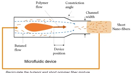
Figure 2: Short polymer fibre production using recirculation.

the ranges overα. When an underspecification is detected, we increment the order of the Bernstein basis. We derive a key lemma to compute the maximum of the derivative for a function realised using Bernstein polynomial basis of a fixed order. Next, using the existing results of order eleva-tion for Bernstein basis, we show how to reuse observaeleva-tion obtained using lower order basis for the new higher order basis. In some cases, it may not be possible to detect order underspecification via derivative checking (if the function has more number of modes than can be modelled by the cur-rent order of the polynomial), and hence, we also increment order at a fixed interval up to a maximum specified order. At all times, we use all the observations using order elevation technique. Convergence is guaranteed as long as the func-tion is realisable within the maximum order specified.

We apply our algorithm to two problems: the design and production of concentrated short polymer fibre solution us-ing recirculation and learnus-ing rate schedule optimisation for neural network training. Interesting new materials like short polymer fibres can impart exotic properties to natural fabrics (Feng et al. 2003; Ma, Hill, and Rutledge 2008). Production involves injecting a liquid polymer into a high speed butanol flow through a specially designed apparatus (Fig 2) (Li et al. 2017). This turns the liquid polymer into short nano-scale fibres. The control variables include the apparatus geometry and flow rates which in turn determine the produced fibre quality. To increase the fibre concentration in the mixture produced, the same mixture (butanol+fibre) is recirculated through the apparatus, keeping the polymer flow uninter-rupted. Since the recirculation process introduces dynamics in the constituents of the mixture, one may need to change the control variables to keep them optimal throughout this dynamic process. We apply our algorithm in maximising the quality of fibre yield for the already mentioned short poly-mer fibre production process. During recirculation we only change the butanol flow rate as a function of time, as others are not easy to change dynamically in the used setup. We used the experimenter’s hunch that an increasing flow rate will result in the highest quality fibre. In our experiments, we found two profiles, one which is nearly constant, and the other which is increasing that both result in the highest qual-ity possible, loosely validating the experimenter’s hunch.

be modelled either as a long vector or as a function of epochs (Bengio 2012). The latter is attractive as the smoothness in the consecutive learning rate values implies smaller effec-tive design space when considered as a function than with a full blown vector of the corresponding schedule. We ap-plied our algorithm for learning rate schedule optimisation and found that an optimised learning rate schedule can even make SGD to perform better than both the method proposed by (Vien, Zimmermann, and Toussaint 2018) and a state of the art optimiser with automatic scheduling like Adam.

Bayesian optimisation

Bayesian optimisation is a global optimisation method for expensive black-box function (Jones, Schonlau, and Welch 1998; Mockus 1994). The optimisation problem:

x∗=argmax_x∈Xf(x)

The function is usually modelled using aGaussian Process

(Rasmussen 2006) as the priori.e.

f(x) ∼ GP(m(x), k(x,x0)).

wherem(x)andk(x,x0_{)are the mean and the covariance}

functions of the Gaussian process (Brochu, Cora, and de Freitas 2010). Mean m(x) can be assumed to be a zero function without any loss of generalisation. Popular co-variance functions include squared exponential (SE) kernel, Mat´ern kernel, etc. The predictive mean and variance of the Gaussian process is a Gaussian distribution, which encap-sulates epistemic uncertainty. Using an observation model of y = f(x) +, where ∼ N(0, σ2

noise), and denoting

D={xi, yi}ti=1, the predictive distribution can be derived

as:

P(ft+1| D1:t,x) =N(µt+1(x), σt2+1(x))

where, k = [k(x,x1), . . . , k(x,xt)], the kernel matrix

[Kij] =k(xi,xj)∀i, j∈1, . . . , t, and

µt+1(x) =kT[K+σnoise2 I]−1y1:t σt+1(x) =k(x,x)−kT[K+σ2noiseI]−1k

Next, a surrogate utility function calledacquisition func-tionis constructed to find the next sample to evaluate. It bal-ances two contrastive needs of sampling at the high mean location versus sampling at the high uncertainty location so that the global optima for f(.)is reached in a fewer num-ber of samples. Acquisition functions are either constructed based on improvement over the current best (e.g. Probabil-ity of Improvement, Expected Improvement (Kushner 1964; Mockus, Tiesis, and Zilinskas 1978)), or information based criteria (e.g. Entropy Search (Hennig and Schuler 2012). Predictive Entropy Search (Hern´andez-Lobato, Hoffman, and Ghahramani 2014)), or confidence based criteria (e.g. GP-UCB (Srinivas et al. 2010)). A GP-UCB acquisition function for the(t+ 1)th iteration is:

at+1(x) =µt(x) + p

βt+1σt(x)

where βt is an increasing sequence of O(log t). An

ex-ample sequence can beβt = 2log(td/2+2π2/3δ)whered

represents the dimensionality of the data and1−δ is the probability of convergence. A regret rt is defined as the

difference of the t’th function evaluation and the global maxima, i.e. rt = maxx∈Xf(x)− f(xt), and the

cu-mulative regret is defined as Rt = P t

t0₌₁rt0. It can be

shown that when Gaussian process is used with SE ker-nel then Rt ∼ O(pt(log t)d+1_{), i.e. the cumulative}

re-gret only grows sublinearly and Limt→∞Rt/t → 0, im-plying a ‘no regret’ algorithm. Generic Bayesian optimi-sation is a sequential algorithm with one recommendation per iteration. However, when at each iteration it is conve-nient to perform a batch of recommendation. it can be al-tered to batch Bayesian optimisation (Contal et al. 2013; Desautels, Krause, and Burdick 2014; Vellanki et al. 2017; Gupta et al. 2018).

Proposed framework

As previously mentioned, we model the control function

g(t)using the Bernstein polynomial basis. Instead of opti-mising the functiong(t)directly, we optimise its Bernstein coefficients{αv}v=1:n. In this manner, we are able to

con-vert our functional optimisation problem into a vector opti-misation problem. In this section, first we present how the optimum control function can be found in the presence of basic shape information. We also discuss how the order of the polynomial can be adjusted based on the complexity of the control function being optimised.

Bernstein polynomial representation with shape

constraints

Annth_{order Bernstein polynomial as a linear combination}

of its basis polynomials is represented as

gn(t) =P n

v=0αvbv,n(t) (1)

wherebv,n(t) = n_v

tv_(1−t)n−v _{are the Bernstein basis}

polynomials for orderndefined on[0,1], n_vis the binomial coefficient, andαv are the Bernstein coefficients. In other words, the Bernstein polynomial is the weighted sum of the basis polynomials. We first present a lemma that guarantees universality of Bernstein polynomial basis.

Lemma 1. (Bernstein 1912). Any continuous function f

defined on the closed interval [0,1]can be uniformly ap-proximated by a Bernstein polynomial functionBn(f). Let Bn(f)(t) = P

n v=0f

v n

bv,n(t). then asn → ∞,Bn(f)

converges to the functionf, i.e.limn→∞Bn(f) =f. @

Next, we present the lemma to control the shape of the function. Our interest lies in the elegant relationship be-tween the Bernstein coefficients{αv}nv=0and the shape of

the Bernstein polynomial. In Theorem 1 and 2, we elaborate on the details of this relationship for the monotonic function and the unimodal function case. The following Lemma leads us towards Theorems 1 and 2.

Lemma 2. For a Bernstein polynomial gn(t) =

Pn

b=0αvbv,n(t), the derivative of the polynomial is given

byg_n0(t) =nPn−1

v=0(αv+1−αv)bv,n−1(t). In other words

Theorem 1. (Monotonicity):Ifαv+1 ≥αv, thengn(t)is a

monotonically increasing function. Similarly ifαv+1≤αv,

thengn(t)is a monotonically decreasing function.(Chang et al. 2007)

Proof. From Lemma 2, consider the derivative of the Bern-stein polynomialg_n0(t) = nPn−1

v=0(αv+1−αv)bv,n−1(t).

Here, the base polynomials{bv,n−1(t)}n−_v=01are always

pos-itive by definition. Therefore, if the difference(αv+1−αv)

is kept positive, the derivativeg0_n(t)remains positive imply-inggn(t)to be a monotonically increasing function. A

sim-ilar argument can be made forgn(x)to be a monotonically decreasing function providedαv+1< αv.

Theorem 2. (Unimodality)(Chang et al. 2007):Forn≥3. Ifα0=α1 =...=αl1 < αl1+1 ≤αl1+2 ≤... ≤αl2 and αl₂ ≥ αl₂+1 ≥ ... ≥ αl3 > αl3+1 = ... = αn for some

0 ≤ l1 < l2 ≤ l3 ≤n, then there exists somes ∈ (0, τ)]

such thatsis the unique maximum point ofgn(t)andgn(t) is strictly increasing on[0, s]and it is strictly decreasing on [s, τ].

Proof. Please refer to (Chang et al. 2007) for proof. The proof also uses Lemma 2 as a key ingredient.

These theorems are used to formulate the constraints in the next subsection. Chang et al. (Chang et al. 2007) have also provided theory for the cases other than unimodal con-cave. Our framework can be extended to all such cases where such a relationship between the coefficients and the shape of the polynomial has been established. Often the prior information about the trend is available from the do-main experts. Specifically, in the design of short polymer fibre, it is known that fibres get shorter as they are recircu-lated. Hence, to get a narrow size-distribution we need to produce longer fibres initially, with a gradual reduction in length. This would require butanol flow to increase mono-tonically with time. On the contrary, for deep learning sched-ule tuning we use monotonically decreasing constraint. Our method can also be applied to applications where the func-tion is either unimodal or even when there is no prior infor-mation available about the shape of the control function.

For illustration, let us consider the functions that are rep-resented via third order Bernstein polynomial basis. The base polynomials in this case are b0,3(t) = (1 − t)3,

b1,3(t) = 3t(1−t)2,b2,3(t) = 3t2(1−t),andb3,3(t) =t3.

Fig 3 shows the sample functions from functions with only range constraint, as well as functions with monotonicty con-straint and unimodality concon-straint.

Control function optimisation with shape

constraints

We recall our optimisation problem as:

x∗_=argmax

x∈Xf(x)

wherex = {α,u},X = A ∪ U,α is the Bernstein co-efficient vector anduare the other fixed control variables. When prior information about the shape of the control func-tion is available, then it boils down to usual constrained op-timisation problem as:

0 0.1 0.2 0.3 0.4 0.5 0.6 0.7 0.8 0.9 1

t 0

0.1 0.2 0.3 0.4 0.5 0.6 0.7 0.8 0.9 1

b0,3(t) b1,3(t) b2,3(t) b3,3(t)

(a) Bernstein base polynomials for the third order Bernstein polynomial.

0 0.5 1 0

0.5

1 random alpha

0 0.5 1 0

0.5

1 increasing alpha

0 0.5 1 0

0.5

1 decreasing alpha

0 0.5 1 0

0.5

1 unimodal alpha

(b) Examples of Bernstein polynomialg3(t)based on how al-phas are sampled.

Figure 3: Examples of a third order Bernstein polynomial.

x∗=argmax_x∈Xf(x) s.t._C≥0

whereCis a set of inequality constraints over the parameter

space. Such constraints can be easily enforced during ac-quisition function optimisation. In the following, we present the _Cfor monotonically increasing and decreasing control functions, and unimodal control functions based on the The-orems 1 and 2.

Controlling the range of the control function: By

choos-ing the values ofα0:n ∈ [0,1]the Bernstein polynomial is

limited to the range [0,1] (this is possible due to Lemma 3, which will be described in the next subsection). For any application, optimised Bernstein polynomial can then be rescaled using the known range of input function.

Increasing control function: C = {Cv}n−v=01 where

Cv =αv+1−αv. This is used in the design of recirculation

control function in short polymer fibre production experi-ment as presented in experiexperi-ments.

Decreasing control function: _C = {Cv}n−v=01 where

Algorithm 1Framework for control function optimisation. Input: Observations D1:m = {xi, yi}mi=1, where yi =

f(gn(t) | xi) +ε for annth order Bernstein polynomial,

xi={αi,ui}forαi ∈R1×n. Fixed increment scheduleω.

Constraints based on shape priorC. form= 1 :M axIteration

buildGPonD1:m

samplexm+1=argmaxx∈Xa(xm|C,D)

evaluateym+1=f(gn(t)|xm+1)(see eq: (1))

obtain the current best sample{x+_{, y}+_}

compute the maximum differencedbetween any ... two coefficients inα+

ifd >0.95ormmodω= 0 update ordern=n+ 1

re-evaluate{αi}mi=1forαi∈R1×(n+1)

update observationsD1:m end if

augment the dataD1:m+1=D1:m∪ {xm+1, ym+1}

end for

learning rate schedules for deep neural network optimisers as presented in experiments.

Unimodal control function: For unimodal control

func-tion we chose simplified constraints adapted from Theo-rem 2. For some0 < l < n, we define the constraints as

C={Cv}n−v=01whereCv=αv+1−αv∀v= 0 :landCv=

αv−αv+1∀v=l:n−1.

Dynamically adjusting order of Bernstein basis

As discussed earlier the intuition is illustrated in Fig 1. We compare the maximum computed derivative of the best con-trol function with the maximum derivative possible with the same order polynomial. If it is close then we increase the polynomial order.

We first derive Lemma 3 that provides an easy way to compute the maximum of the derivative of a function based on the Bernstein coefficients.

Lemma 3. The derivativeg0n(t)of the Bernstein

polyno-mial of order ngn(t)is bounded by ‘n’ times the maxima of the basis polynomial with the highest coefficient.

Proof. It can be said about Bernstein polynomials that the range of the polynomialgn(t)is bounded by the values of

the minimum and maximum values of the Bernstein coef-ficients {αv}v=0:n. Then from Lemma 2 we can say that

the derivative of the Bernstein polynomialg_n0(t)is bounded by the values of the minimum and maximum of the val-ues of the Bernstein coefficients{n(αv+1−αv)}v=0:n−1.

By the same token the theoretical maximum of the mag-nitude of the derivative is(αmax−αmin), assumingα ∈

[αmax, αmin].

Based on this it can be said that ann-th order Bernstein polynomial can only be used to sufficiently approximate a function if the derivate of the function is within the bounds as stated in Lemma 3. We should test whether the current function has already reached the limit or at least close to it. If it is true then we can decide that the current order is underspecified and we increment the order by one.

Next, we use the following lemma to reuse the past ob-servations by transforming{αv}v=0:nvectors of lengthnto

{α0_v}v=0:n+1vectors of lengthn+ 1.

Lemma 4. A Bernstein polynomial of ordern and with Bernstein coefficients {αv}v=0:n can be represented

us-ing a Bernstein polynomial of order n+ 1with Bernstein coefficients {α0_v}v=0:n+1, such that α

0

v = n+1v αv−1 +

1− v n+1

αv. In other words, it is possible to raise the

or-der of the Bernstein polynomial and recompute the Bern-stein coefficients.(Please refer to (Lorentz 2012)) @

Lemma 3 can detect one type of signs of underspecifica-tion. To avoid underspecification altogether, we also incre-ment the order at a regular interval until a maximum spec-ified order is reached. The overall algorithm is presented in Algo 1. If the order of the Bernstein polynomial be-comes very high then it is possible to use high-dimensional Bayesian optimisation (Rana et al. 2017; Oh, Gavves, and Welling 2018).

Experiments

We evaluate our proposed functional optimisation method on one synthetic and two real world experiments: optimi-sation of fibre yield in short polymer fibre production, and learning rate schedule optimisation for neural network train-ing. For convenience, we refer to the proposed algorithm as BFO-SP. For all experiments, we start with a 5th order Bern-stein polynomial basis, but limit the highest order to 10. The change of order is triggered due to hitting the derivative limit when it reaches 95% of the maximum derivative magni-tude possible. The code will be made available upon request. Given a problem, the shape prior is an estimation of the field expert. For example, in the application of short polymer fi-bre design, our material science collaborators know from the fluid dynamics principles that the shape of the function needs to have an increasing flow profile for optimal produc-tion of fibres. It is this hunch that has been incorporated into the optimisation system. In a scenario where such a hunch is unavailable we would have used the general form of BFO without the shape prior constraint.

1 2 3 4 5 6 7 8 9 10

t

0 0.2 0.4 0.6 0.8 1

g(t)

Optimal

Best with degree = 5 Final best (degree = 8) Final best (Vien et al. 2018)

(a) With monotonicity constraint.

1 2 3 4 5 6 7 8 9 10

t

0 0.2 0.4 0.6 0.8 1 1.2

g(t)

Optimal

Best with degree = 5 Final best (degree = 9) Final best (Vien et al. 2018)

(b) With unimodality constraint.

Figure 4: Synthetic experiment.

Synthetic experiments

In the synthetic experiment, we construct two different 10 dimensional vectors, one which is monotonically decreas-ing and the other which is unimodal convex. These can be thought of schedule vectors, sampled on a fixed grid of size 10 from the optimal control functions that we would like to recover via our functional optimisation approach. For each, the utility of a trial control function is measured by first sam-pling the control function on the same grid and evaluating the resultant 10 dimensional vector through a Gaussian pdf function whose mean is the respective optimal vector.

We start with Bernstein polynomial of order 5 and then increase the order when either a) at the trigger as mentioned in Lemma 2, or b) at a fixed schedule of every 10 iterations. The results are shown in Fig 4 with a) showing the case for monotonicity and b) showing the case for unimodality. In the plots we show the optimal (in red), the best so far when the first order change is triggered by lemma 2 (in teal) and the best one after 20 iterations. For both the cases order changes have been triggered multiple times resulting in the final best with a considerable higher order (8 for monotonicity and 9

0 1 2 3 4 5 6 7 8

time 0

10 20 30 40

butanol flow

g1(t) g2(t) baseline

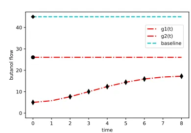
Figure 5: Short polymer fibre production: Best recircula-tion control funcrecircula-tions g(t)found compared to baseline.

g1(t)andg2(t)gave highest score (9).

for unimodality). The final best ones appear much closer to the optimal one. The results are compared with the method proposed by (Vien, Zimmermann, and Toussaint 2018) (in green), where incorporating prior is not possible.

Short polymer fibre production

We optimise the butanol flow profile over the recirculation period to achieve a high quality yield of concentrated fibres. All other variables (device geometry and polymer flow) are fixed to the known best setting. The recirculation is run till a fixed time, limited by the maximum concentration achiev-able with the chosen polymer flow. At the end of each exper-iment a sample of fibre is looked at under a powerful optical microscope to inspect fibre length and diameter distribution. Quality score is given between 1-10, with 10 being the high-est for fibre distribution with small variance. Experimenters had a hunch that an increasing flow profile will result in a higher quality yield, which we used as our shape prior. We used GP-UCB-PE with batch size of 6.

We have been able to reach a score of 9 out of a max-imum score of 10, within 5 iterations. Fig 5 shows exam-ples of butanol flow schedules for which high scores were recorded. Both a flat and increasing profile results in a score of 9, thus validating the experimenter’s hunch. These are im-provements over their current baseline with a fixed butanol flow (8). The markers on each function are time intervals at which the butanol flow is changed.

Learning rate schedule optimisation

Dataset Validation error

BFO-SP + SGD SGD Adam BFO + SGD (Vien et al. 2018)

CFIR10 18.81% 20.30% 20.20% 22.2%

MNIST 0.74% 1.26% 0.86% 0.87%

Table 1: Comparison of prediction error of Bayesian optimisation of learning rate schedule against SGD and Adam with exponential decay for both CFIR10 and MNIST datasets.

0 1 2 3 4 5 6 7 8 9

epoch number 0.01

0.02 0.03 0.04 0.05 0.06 0.07

leanring rate

CFIR10 LR Schedule MNIST LR Schedule

Figure 6: Learning rate schedules that resulted in the highest accuracy on CFIR10 and MNIST datasets using the BFO-SP with known prior - monotonicity constraint.

0 1 2 3 4 5 6 7 8 9 10 11 12 13 14 epoch number

0.000 0.025 0.050 0.075 0.100 0.125 0.150 0.175 0.200

leanring rate

CFIR10 LR Schedule MNIST LR Schedule

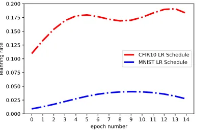
Figure 7: Learning rate schedules that resulted in the highest accuracy on CFIR10 and MNIST datasets using (Vien, Zimmermann, and Toussaint 2018)

For CFIR10 we use a network architecture that be sum-marised as (Conv2D → Dropout → Conv2D →

M axpooling2D) × 3 → F latten → (Dropout →

Dense)×3. Whereas for MNIST the network architecture used is (Conv2D → M axpooling2D → Dropout →

F latten→Dense→Dense). (Details about the network architecture are given in the supplementary material). Fig 6 shows the optimised learning schedules for CFIR10 and MNIST datasets using the proposed method. For Bayesian optimisation the range of learning rate was chosen between 0.2 and 0.0001. For Adam and SGD the starting learning rate used was 0.01, with 0.8 momentum for SGD and default values for hyper-parameters of Adam (Kinga and Adam 2015). We compare the performance of learning rate

opti-mised stochastic gradient descent (SGD) optimiser against a) SGD with an exponential decay and b) Adam. Tab 1 shows the performance comparison with the baselines af-ter 20 Bayesian optimisation iaf-teration. On both the datasets our method BFO-SP achieved higher performance than the baselines. The results are also compared with BFO by (Vien, Zimmermann, and Toussaint 2018) as shown in Fig 7. By ad-mitting prior knowledge, our proposed method turns out to be the most efficient .

Conclusion

We present a novel approach for functional optimisation with Bayesian optimisation. We use Bernstein polynomials to model the control function and in turn optimise the Bern-stein coefficients to learn the optimum function shape. Prior shape information (e.g. monotonicity, unimodality etc) is in-tegrated and the polynomial order is dynamically adjusted during the optimisation process. We demonstrate the perfor-mance of our method by applying it for short polymer fi-bre production via a recirculating process, and for modelling learning rate schedule for deep learning networks. For fibre production we use monotonically increasing prior, whereas for deep networks we use monotonically decreasing shape prior. Our method outperform baselines in all the cases.

Currently, the method proposed is built to work for uni-modal and increasing or decreasing shape priors. A natural progression is to extend this for other complex shape pri-ors (eg. multimodal) as well. It would also be interesting to consider multi-variate Bernstein polynomial when multiple variables may form inter-related function of time. An inte-gration of stable Bayesian optimisation (Dai Nguyen et al. 2017) will be important for industrial applications. It would be interesting to analyse how variation in the final schedule dictates variation in the coefficients of the Bernstein polyno-mials. The proposed method can be applied in a variety of domains including plastic recycling industry, drug manufac-turing and even in alloy heat treatment optimisation where the usual process of constant temperature heat treatment can be replaced by a variable temperature treatment to achieve faster result with possibly lower energy usage.

Acknowledgement

References

Bengio, Y. 2012. Practical recommendations for gradient-based training of deep architectures. InNeural networks: Tricks of the trade. Springer. 437–478.

Bernstein, S. 1912. Demonstration of a theorem of weierstrass based on the calculus of probabilities. Com-munications of the Kharkov Mathematical Society Volume XIII(1912/13):1–2.

Brochu, E.; Cora, V. M.; and de Freitas, N. 2010. A tuto-rial on Bayesian optimization of expensive cost functions, with application to active user modeling and hierarchical re-inforcement learning.arXiv:1012.2599.

Chang, I.-S.; Chien, L.-C.; Hsiung, C. A.; Wen, C.-C.; and Wu, Y.-J. 2007. Shape restricted regression with random bernstein polynomials. Lecture Notes-Monograph Series

187–202.

Contal, E.; Buffoni, D.; Robicquet, A.; and Vayatis, N. 2013. Parallel Gaussian process optimization with upper confi-dence bound and pure exploration. InJoint European Con-ference on Machine Learning and Knowledge Discovery in Databases, 225–240. Springer.

Dai Nguyen, T.; Gupta, S.; Rana, S.; and Venkatesh, S. 2017. Stable Bayesian optimization. InPacific-Asia Conference on Knowledge Discovery and Data Mining, 578–591. Springer. Desautels, T.; Krause, A.; and Burdick, J. W. 2014. Paral-lelizing exploration-exploitation tradeoffs in Gaussian pro-cess bandit optimization. Journal of Machine Learning Re-search15(1):3873–3923.

Feng, L.; Song, Y.; Zhai, J.; Liu, B.; Xu, J.; Jiang, L.; and Zhu, D. 2003. Creation of a superhydrophobic surface from an amphiphilic polymer. Angewandte Chemie International Edition42(7):800–802.

Gupta, S.; Shilton, A.; Rana, S.; and Venkatesh, S. 2018. Exploiting strategy-space diversity for batch bayesian opti-mization. In Storkey, A., and Perez-Cruz, F., eds., Proceed-ings of the Twenty-First International Conference on Artifi-cial Intelligence and Statistics, volume 84 ofProceedings of Machine Learning Research, 538–547. Playa Blanca, Lan-zarote, Canary Islands: PMLR.

Hennig, P., and Schuler, C. J. 2012. Entropy search for information-efficient global optimization. Journal of Ma-chine Learning Research13:1809–1837.

Hern´andez-Lobato, J. M.; Hoffman, M. W.; and Ghahra-mani, Z. 2014. Predictive entropy search for efficient global optimization of black-box functions. InAdvances in neural information processing systems, 918–926.

Jones, D. R.; Schonlau, M.; and Welch, W. J. 1998. Effi-cient global optimization of expensive black-box functions.

Journal of Global optimization13(4):455–492.

Kinga, D., and Adam, J. B. 2015. A method for stochas-tic optimization. InInternational Conference on Learning Representations (ICLR), volume 5.

Kulfan, B., and Bussoletti, J. 2006. ” Fundamental” pa-rameteric geometry representations for aircraft component shapes. In11th AIAA/ISSMO multidisciplinary analysis and optimization conference, 6948.

Kushner, H. J. 1964. A new method of locating the max-imum point of an arbitrary multipeak curve in the presence of noise. Journal of Basic Engineering86(1):97–106. Li, C.; de Celis Leal, D. R.; Rana, S.; Gupta, S.; Sutti, A.; Greenhill, S.; Slezak, T.; Height, M.; and Venkatesh, S. 2017. Rapid bayesian optimisation for synthesis of short polymer fiber materials. Scientific reports7(1):5683. Li, C.; Rana, S.; Gupta, S.; Nguyen, V.; Venkatesh, S.; Sutti, A.; Rubin, D.; Slezak, T.; Height, M.; Mohammed, M.; and Gibson, I. 2018. Accelerating experimental design by in-corporating experimenter hunches. InData Mining (ICDM), 2018 IEEE International Conference on, 1–8. IEEE. Lorentz, G. G. 2012. Bernstein polynomials. American Mathematical Soc.

Ma, M.; Hill, R. M.; and Rutledge, G. C. 2008. A re-view of recent results on superhydrophobic materials based on micro-and nanofibers. Journal of Adhesion Science and Technology22(15):1799–1817.

Mockus, J.; Tiesis, V.; and Zilinskas, A. 1978. The appli-cation of Bayesian methods for seeking the extremum. To-wards Global Optimization2:117–129.

Mockus, J. 1994. Application of bayesian approach to nu-merical methods of global and stochastic optimization. Jour-nal of Global Optimization4(4):347–365.

Oh, C.; Gavves, E.; and Welling, M. 2018. BOCK : Bayesian optimization with cylindrical kernels. In Dy, J., and Krause, A., eds.,Proceedings of the 35th International Conference on Machine Learning, volume 80 of Proceed-ings of Machine Learning Research, 3868–3877. PMLR. Rana, S.; Li, C.; Gupta, S.; Nguyen, V.; and Venkatesh, S. 2017. High dimensional Bayesian optimization with elastic Gaussian process. In Precup, D., and Teh, Y. W., eds., Pro-ceedings of the 34th International Conference on Machine Learning, volume 70 ofProceedings of Machine Learning Research, 2883–2891. PMLR.

Rasmussen, C. E. 2006. Gaussian processes for machine learning.

Samareh, J. A. 2001. Survey of shape parameterization tech-niques for high-fidelity multidisciplinary shape optimiza-tion. AIAA journal39(5):877–884.

Srinivas, N.; Krause, A.; Kakade, S.; and Seeger, M. W. 2010. Gaussian process optimization in the bandit set-ting: No regret and experimental design. In Proceedings of the 27th International Conference on Machine Learning (ICML-10), 1015–1022.