Learning Diffusions without Timestamps

(1)

The Thirty-Third AAAI Conference on Artificial Intelligence (AAAI-19)

Learning Diffusions without Timestamps

Hao Huang,

1

_{Qian Yan,}

1

_{Ting Gan,}

1

_{Di Niu,}

2

_{Wei Lu,}

3

_{Yunjun Gao}

4

1_{School of Computer Science, Wuhan University, China}

2_{Department of Electrical and Computer Engineering, University of Alberta, Canada} 3_{School of Information and DEKE, MOE, Renmin University of China, China}

4_{College of Computer Science and Technology, Zhejiang University, China}

{haohuang, qy, ganting}@whu.edu.cn, [email protected], [email protected], [email protected]

Abstract

To learn the underlying parent-child influence relationships between nodes in a diffusion network, most existing ap-proaches require timestamps that pinpoint the exact time when node infections occur in historical diffusion processes. In many real-world diffusion processes like the spread of epidemics, monitoring such infection temporal information is often expensive and difficult. In this work, we study how to carry out diffusion network inference without infection timestamps, using only the final infection statuses of nodes in each historical diffusion process, which are more readily accessible in practice. Our main result is a probabilistic model that can find for each node an appropriate number of most probable parent nodes, who are most likely to have generated the historical infection results of the node. Exten-sive experiments on both synthetic and real-world networks are conducted, and the results verify the effectiveness and efficiency of our approach.

Introduction

In real life, many underlying influence relationships among people form various diffusion networks, spreading different contents such as information, viewpoints, or even viruses. Diffusion network inference aims to uncover these influ-ence relationships based on the spread results observed in historical diffusion processes. Therefore, this problem is fundamental in many applications such as information propagation (He et al. 2015), viral marketing (Leskovec, Adamic, and Huberman 2007), and epidemic prevention (Wallinga and Teunis 2004), in which the inferred influence relationships can intuitively illustrate the latent diffusion paths, and help users to better predict, promote or prevent future diffusion events.

Most existing approaches to diffusion network inference are based on the following basic ideas: nodes that are infected sequentially within a time interval are assumed to have influence relationships, and the previously infected ones are regarded as potential parent nodes of the subse-quently infected ones. Hence, these approaches require the observed spread results used by them (known as cascades) to include the exact infection timestamps of the infected nodes in each diffusion process. To infer diffusion networks

with given cascades, a major method is adopting a con-vex optimization framework to find influence relationships that maximize the likelihood of the cascades, and utiliz-ing techniques, such as sequential quadratic programmutiliz-ing (Myers and Leskovec 2010; Gomez-Rodriguez, Balduzzi, and Schölkopf 2011), block coordinate descent (Du et al. 2012), stochastic and proximal gradient methods (Gomez-Rodriguez, Leskovec, and Schölkopf 2013b; Daneshmand et al. 2014), survival theory (Gomez-Rodriguez, Leskovec, and Schölkopf 2013a), EM algorithm (Wang et al. 2014; Rong, Zhu, and Cheng 2016), and sparse recovery (Pouget-Abadie and Horel 2015), to approximate the optimal solution. While several other approaches adopt non-convex optimization frameworks, each of them finally decouples the non-convex problem into multiple smaller convex problems (Netrapalli and Sanghavi 2012; Narasimhan, Parkes, and Singer 2015; Kalimeris et al. 2018). Another effective method is trans-forming the problem of diffusion network inference into that of submodular optimization (Gomez-Rodriguez, Leskovec, and Krause 2010; Gomez-Rodriguez and Schölkopf 2012) by constructing a likelihood function of cascades with the property of submodularity. Then, a near-optimal solution of the submodular optimization problem can be achieved by applying greedy algorithm. It has been validated that with adequate amount of complete and correct cascades, the influence relationships can be accurately recovered, even using some simple inference approaches (Abrahao, Chierichetti, and Kleinberg 2013). In addition, some more sophisticated approaches are proposed to handle the case that cascades have partial incorrect infection timestamps (Sefer and Kingsford 2015) or miss partial snapshots of the network (He et al. 2016; Lokhov 2016).

(2)

occurrence time of infections.

To avoid the limitation of cascade-based approaches, new techniques are required to learn diffusions without the infection timestamps. To the best of our knowledge, only two existing works have partially addressed this problem by learning either from path traces (referred to as PATH henceforth) or from the seed and resulting sets of infected nodes (referred to as S2R henceforth). In PATH (Gripon and Rabbat 2013), the learner is assumed to have all path-connected triples, i.e., three nodes that are activated along a diffusion path through the network. Although PATH has a solid mathematical foundation, the triples are not al-ways naturally observable in practice. Even if complete and correct cascades are available, inferring exact triples is still challenging. S2R (Amin, Heidari, and Kearns 2014) calculates the lifting effect of each seed nodeuto another infected nodev, which measures the increase in the proba-bility ofv’s infection on the condition thatuis previously infected. Then, S2R adds a directed edge (i.e., an influence relationship) from u to v, if u has the greatest current lifting effect tov. It’s worth noting that if there is no priori knowledge on the number of edges in the network, S2R will keep adding edges until all nodes are connected.

Aiming at a more general solution to diffusion learn-ing, in this paper, we study the problem of how to infer diffusion networks with only the final infection statuses of the nodes in historical diffusion processes, which are more readily accessible in practice. We propose an effective and efficient algorithm called TWIND (DiffusionNetwork

InferenceWithoutTimestamps) for this problem. TWIND reveals potential parent-child influence relationships by find-ing for each node a set of most probable parent nodes, who are most likely to have generated the observed infection results. To this end, we present a probabilistic model to quantify the possibility of inferred influence relationships given the observed final infection statuses. Based on the model, we can also theoretically derive an upper limit on the amount of most probable parent nodes for each node in the network, which helps TWIND to prevent its inferred diffusion network from containing too many low-probability influence relationships not in the original diffusion net-work. Furthermore, to reduce redundant computation during the execution of TWIND, we disqualify the insignificant candidate parent nodes whose infections have rather weak correlations with the infections of the corresponding child nodes, and exclude them from the selection of most probable parent nodes.

In summary, our key contributions include the following: (1) We propose a new infection timestamp-free approach for diffusion network inference. To execute this approach, there is no need to monitor the infection timestamps of nodes through each diffusion process, or to worry about the correctness of observed infection timestamps. Except for the final infection statuses of nodes, the approach does not need any other information of infections or priori knowledge on the network. (2) We theoretically guarantee that TWIND will find for each node an limited number of most probable parent nodes, avoiding an overly complex inferred network. In what follows, we first present our problem statement,

and then elaborate our proposed TWIND algorithm, fol-lowed by reporting experimental results and our findings before concluding the paper.

Problem Statement

A diffusion network can be represented as a directed graph

G = {V, E}, where V = {v1, v2, ..., vn} is the set of n

nodes in the network, andEis the set ofmdirected edges (i.e., influence relationships) between the nodes. A directed edge from a parent nodevito a child nodevjindicates that

whenviis infected andvjis uninfected,viwill successfully infectvj with a certain probability (which can be regarded as the edge weight of this directed edge). As a few existing approaches have presented how to calculate the edge weight based on observed infection status results for a specified edge (Yan et al. 2017), in this paper, we focus on inferring the unknown directed edge set of the objective network. Our problem can be formulated as follows.

Given:a setS ={S1_{, ..., S}β_}_{of infection status results}

observed on a diffusion networkGinβdiffusion processes, where Sℓ ₌ _{sℓ

1, ..., sℓn} is a n-dimensional vector that

records the final infection statussℓ

i ∈ {0,1}(1 for infected

status and 0 for uninfected status) of each node vi ∈ V

observed in theℓ-th diffusion process (ℓ∈ {1, . . . , β}).

Infer:the edge setEof the diffusion networkG.

The TWIND Algorithm

In this section, we first introduce how to identify the most probable parent nodes for each node in the network, fol-lowed by a theoretical analysis of the upper limit on the amount of most probable parent nodes, and then we present how to reduce redundant computation during the identifica-tion of most probable parent nodes before giving the detailed steps of our TWIND algorithm. We conclude this section with a complexity analysis on our approach.

Identification of Most Probable Parent Nodes

Let matrix A ∈ Rn×n be a network structure variable, of which each elementAij ∈ {0,1}(i, j ∈ {1, . . . , n})

indi-cating whether there is a directed edge from nodevito node

vj (1 for yes,0 for no), diffusion network inference using

infection status resultsS is equivalent to finding a optimal

Athat maximizes the following conditional probability:

P(A|S) =_∑ P(A, S)

A′_∈_QP(A′, S)

(1)

where setQis the set of all possible matrices ofA, and the value of∑

A′_∈_QP(A′, S)is a certain constant. Maximizing

probabilityP(A | S)is equivalent to maximizing the joint probabilityP(A, S), which can be calculated as follows.

P(A, S) = ∫

B

P(S|A, B)f(B|A)P(A)dB

=P(A)

∫

B

P(S|A, B)f(B|A)dB

(2)

whereB is an×nblock matrix related toA. IfAij = 0,

(3)

2×2nonnegative matrix, of which each element refers to a conditional probabilityP(Xj |Xi)_>0, whereXi∈ {0,1}

andXj ∈ {0,1}are the infection status variables of nodes viandvj, respectively.

Since each historical diffusion process is independent to each other, eachSℓ _{is generated independently. Moreover,}

since the infection of each node can be only affected by its parent nodes during each diffusion process, the relationship

P(X1, . . . , Xn) = ∏n

i=1P(Xi | XFi)holds, whereFi is the parent node set of nodevi, andXFiis the infection status variables of the parent nodes ofvi. Then, we can reformulate the probabilityP(S|A, B)in Eq. (2) as follows.

P(S|A, B) =∏β

ℓ=1P(S ℓ

|A, B)

=∏β

ℓ=1P(X1=s ℓ

1, . . . , Xn=sℓn|A, B)

=∏β

ℓ=1

∏n

i=1P(Xi=s ℓ

i|XFi=π

ℓ i, B)

=

n

∏

i=1 2|Fi|

∏

j=1 2

∏

k=1

P(Xi=sk|XF_i=πij, B)Nijk

=

n

∏

i=1 2|Fi|

∏

j=1 2

∏

k=1 θNijk

ijk

(3)

where πℓ_i refers to the infection statuses of vi’s parent nodes in the ℓ-th diffusion process, sk ∈ {0,1} is the

k-th possible infection status of a node (without loss of generality,s1 = 0, s2= 1),2|Fi|_{refers to the number of all} possible combinations of the infection statuses ofvi’s parent nodes,πij is the correspondingj-th possible combination, Nijkis the number of times situationXi=sk∧XF_i =πij

appears inS,θijkis equal toP(Xi =sk |XFi =πij, B), and∀vi,∑2|Fi|

j=1

∑2

k=1Nijk=β,θij1+θij2= 1.

Letf(θij1, θij2)denote the probability density function of (θij1, θij2). Since there is no correlation between the influences of different parent nodes to a same child node (or a same parent node to different child nodes), relationship

f(B|A) = ∏n

i=1

∏2|Fi|

j=1 f(θij1, θij2)holds. Combining it

with Eq. (3), we can reformulate the calculation of probabil-ityP(A, S)as follows.

P(A, S)

=P(A)

∫

B

⎛

⎝ (

∏n

i=1

∏2|Fi|

j=1

∏2

k=1θ Nijk

ijk

)

×(∏n

i=1

∏2|Fi|

j=1 f(θij1, θij2)

) ⎞

⎠dB

=P(A)

n

∏

i=1 2|Fi|

∏

j=1

∫ ∫

θij1,θij2

( ∏2

k=1θ Nijk

ijk ×f(θij1, θij2)

)

dθij1dθij2

(4) As there is no prior knowledge on the value ofθijk, we

are indifferent to regard every possible value ofθijk. In other words, we assume that distributionf(θij1, θij2)is uniform,

for 1 ₆ i ₆ n, 1 ₆ j ₆ 2|Fi|_{. Then, the value of}

f(θij1, θij2), denoted ascij, is a constant. According to the

property of probability density function, we have

∫ ∫

θij1,θij2

f(θij1, θij2)dθij1dθij2

= ∫ ∫

θij1,θij2

cijdθij1dθij2= 1

(5)

According to Dirichlet’s integral, we have

∫ ∫

θij1,θij2

dθij1dθij2=

1

(2−1)! = 1 (6)

∫ ∫

θij1,θij2

( ₂

∏

k=1 θNijk

ijk

)

dθij1dθij2

= Nij1!·Nij2!

(Nij1+Nij2+ 2−1)!

(7)

Combining Eqs. (5) & (6), we havef(θij1, θij2) = cij =

1. Combining this conclusion with Eq. (7), we can finally formulate the calculation of probabilityP(A, S)as follows.

P(A, S) =P(A)

n

∏

i=1 2|Fi|

∏

j=1

Nij1!·Nij2!

(Nij1+Nij2+ 1)! (8)

To estimate P(A, S), we need a prior probabilityP(A)

for each possible network structure, and the numbers Nij1

andNij2determined by each nodeviand its parent nodes

Fi in corresponding network structure.Nij1 andNij2 can be counted from the observed infection status results S, while there is no prior knowledge on the network structure to estimateP(A). Furthermore, as there are 2n(n−1)_possible

network structures, it is not feasible to apply Eq. (8) for each possible network structure whenn is large. Therefore, we equally treat each possible network structure by assuming equal priors onA, i.e., the prior probabilityP(A)is equal to a certain constant. Then, to maximizeP(A, S), what we need to do is finding for each nodevia optimal parent node

setFithat maximizes the following scoring function.

g(vi, Fi) = log

2|Fi|

∏

j=1

Nij1!·Nij2!

(Nij1+Nij2+ 1)!

=

2|Fi|

∑

j=1

(

logNij1! + logNij2!

−log(Nij1+Nij2+ 1)!

)

(9)

where the base oflogis 2. Then, the nodes in this optimal

Fiare regarded as the most probable parent nodes ofvi. Given the above scoring function, we can utilize greedy search to find the most probable parent nodes for vi. It starts from an empty parent node setFi, and expands the setFi by incrementally adding a node combination (i.e., a subset ofV\{vi}) that can most increase the value of current

g(vi, Fi)until this value dose not increase. In this way, we

(4)

Upper Limit on Amount of Parent Nodes

At the beginning of the greedy search for most probable parent nodes of a nodevi,Fi =∅and currentg(vi, Fi)can

be calculated as follows.

g(vi,∅) =∑2

k=1logNik!−log(β+ 1)! (10)

whereNikis the number of times situationXi=skappears inS, and∑2

k=1Nik = β. Since( N

e)

N _{< N}_! _{< e}₍N 2)

N

always holds for any positive integerN, we can deduce a lower bound on the value ofg(vi,∅)as follows.

g(vi,∅)> 2

∑

k=1

log

(_N

ik e

)Nik

−loge

(_β_{+ 1}

2

)β+1

=

2

∑

k=1

NiklogNik

e −loge−(β+ 1) log

β+ 1 2

=

2

∑

k=1

Niklogβ

e +β 2

∑

k=1 Nik

β log Nik

β −loge

−(β+ 1) logβ+ 1

2

=βlogβ

e −βH(Xi)−loge−(β+ 1) log

β+ 1 2

(11)

whereH(Xi)is the entropy of variableXi.

When the greedy search method adds a few nodes into set

Fi(i.e.,Fi̸=∅), the following inequality should hold. g(vi, Fi)> g(vi,∅) (12)

Moreover, although there are2|Fi|_{possible combinations} of the infection statuses of nodes inFi, some combinations may not have instances in the observed infection status results S. We denote the number of these non-existent combinations as δi. It can be obtained by checking how

many of the 2|Fi| _{possible combinations have instances in}

S. As each of these existent combinations has at least one instance inS, i.e.,Nij1+Nij2>1, we can have relationship

∑2|Fi|

j=1 log(Nij1+Nij2+ 1) >

∑2|Fi|−δi

j=1 log(1 + 1). In

addition, given the fact that N! ₆ NN_{, we can deduce a}

upper bound on the value ofg(vi, Fi)as follows.

g(vi, Fi)6 2|Fi|

∑

j=1

( ₂

∑

k=1

logNijkNijk

)

− 2|Fi|₋_δ

i

∑

j=1

log 2

=

2|Fi|

∑

j=1 2

∑

k=1

Nijklog (

βNijk β

)

−(2|Fi|₋_δi₎

=

2|Fi|

∑

j=1 2

∑

k=1

Nijklogβ−2|Fi|₊_δi

−

⎛

⎝−β

2|Fi|

∑

j=1 2

∑

k=1 Nijk

β log Nijk

β

⎞

⎠

=βlogβ−2|Fi|₊_δi₋_βH₍_{Xi, XF} i)

(13)

whereH(Xi, XFi)is the entropy of variablesXiandXFi. Combining Eqs. (11)–(13), we have relationship

βlogβ−βH(Xi, XFi)−2

|Fi|₊_δi

> βlogβ

e −βH(Xi)−loge−(β+ 1) log

β+ 1 2

(14)

which can be translated as

2|Fi|_<₍_β_{+ 1) log}

(

eβ+ 1

2 )

+δi−βH(XF_i|Xi)

(15) whereH(XF_i|Xi) =H(Xi, XF_i)−H(Xi)is the entropy ofXFiconditioned onXi. As relationshipH(XFi|Xi)>0 always holds, we have

|Fi|<log (

(β+ 1) log

(

eβ+ 1

2 )

+δi

)

(16)

Therefore, by using the greedy search method to find a setFi

of most probable parent nodes for a nodevi, the upper limit ηfor the set size ofFiislog((β+ 1) log(eβ+1₂ )+δi). In practice, if there is enough historical data logged inS, i.e.,

β ≫δi, we can adopt a fast estimation on the value ofηby

usingη=⌈log((β+ 1) log(eβ+1₂ ))⌉.

Based on thisη, each possible node combination that has the chance to be added into current Fi should satisfy the condition that when this node combination is added into currentFi, the size of newFiwill not be greater thanη.

Pruning of Candidate Parent Nodes

In a given diffusion network with a node setV, each node

vj ∈ V\{vi} could be a candidate parent node for node

vi ∈ V, resulting in ∑η

i=1

( i

n−1

)

possible parent node combinations forvi, wherenis the number of nodes inV. To avoid redundant computation, we should prune the candidate parent nodes to reduce the number of possible parent node combinations for each nodeviin the network.

Given the fact that the infections of nodes are affected by their parent nodes, the infection statuses of the parent nodes and corresponding child nodes should have correlation. In other words, if the infection statuses of two nodes are independent or have extremely low correlation to each other, there is a very low probability that these nodes have influ-ence relationship between them. To quantify the correlation between two variables, mutual information (abbreviated as

M I) is a commonly used criterion and can be calculated as

M I(Xi, Xj) =P(Xi, Xj) log P(Xi, Xj)

P(Xi)P(Xj)

. (17)

A greater value of M I(Xi, Xj) indicates a stronger cor-relation between the infection statuses of nodes vi andvj. Furthermore, in a real-world diffusion network, each node

vi often has a finite number of parent nodes. Many other

nodes in this network do not have influence relationships to

vi, and their infection statuses often have no (or very low)

(5)

Algorithm 1:The TWIND Algorithm

Input :Node setV ={v1, . . . , vn}, infection status

resultsS ={S1_{, . . . , S}β_}_{observed on}_V_. Output:The diffusion networkG={V, E}.

1 E=∅; // the set of directed edge

2 ∀vi∈V, vj∈V, calculateM I(Xi, Xj)by Eq. (17); 3 Partition allM Ivalues into two groups byK-means

(withK= 2and one mean fixed to 0), and setτto the greatestM Ivalue in the group with mean closer to 0;

4 η =

⌈

log((β+ 1) log(eβ+1₂ ))⌉; //|Fi|’s upper limit

5 for eachv_i∈V do

6 Fi=∅; // inferred parent node set ofvi 7 Pi=∅; // candidate parent node set ofvi 8 Ci=∅; //set of possible parent node combinations

9 for eachvj∈V(j ̸=i)do

10 if M I(Xi, Xj)> τ then

11 Pi=Pi⋃{vj}; // mergevjintoPi

12 for eachW ⊆Pi,|W|6ηdo

13 Calculateg(v_i, W)by Eq. (9);

14 Ci={Ci, W}; // add a new elementW toCi

15 while Ci̸=∅do

16 W∗= arg max

W∈Ci

g(vi, W);

17 if |Fi⋃W∗|6ηthen

18 F_i=F_i⋃W∗;

19 Ci=Ci\W∗;

20 E={(vj, vi)|vj ∈Fi}⋃E; //(vj, vi)is directed

Inspired by this kind of situations, we can carry out a heuristic pruning method to screen out insignificant candi-date parent nodes for each node. As the very small M I

values form a compact cluster with a mean close to 0, we can executeK-means withK= 2and fix one of the two means to 0 through all the iterations ofK-means. This modifiedK -means algorithm can efficiently partition allM Ivalues into two groups, in which one group has a mean very close to 0. Letτ be the greatestM Ivalue in the group with a mean closer to 0, then for eachM I(Xi, Xj) ₆τ, we regard the corresponding nodevj as an insignificant candidate parent

node forvi, and exclude it from the candidate parent node set ofvi, since the very smallM Ivalue means that there is

a high probability thatvjhas no influence relationship tovi.

Algorithm

To infer a diffusion network with observed infection status resultsS, we introduce how to identify the most probable parent nodes for each node in the network, deduce an upper limit on the amount of most probable parent nodes, and present a heuristic pruning method to help avoid redundant computation during the identification of most probable par-ent nodes. Based on these preparing work, we propose an algorithm called TWIND, which is outlined in Algorithm 1. TWIND takes as inputs node set V of the objective

diffusion network Gand a setS of infection status results observed on V in β diffusion processes, and consists of two main phases, i.e., (1) the phase of pruning candidate parent nodes, which calculates the M I value for each node pair by Eq. (17) (lines 2), and performs K-means to select candidate parent nodes with greater M I values (lines 3, 9–11), and (2) the phase of greedy search for the parent node set Fi of each node vi (lines 12–20), which first traverses all possible parent node combinations and calculates corresponding scores by scoring function proposed in Eq. (9) (lines 12–14), and then continuously expands the parent node set Fi with the highest scored

parent node combinations until the size of Fi is equal to the upper boundηor there is no more possible parent node combination (lines 15–19). Finally, a directed edge from each node in Fi tovi will be added into the inferred edge

setEof the objective diffusion networkG(line 20).

Complexity Analysis

In TWIND, the most computationally expensive process consists of the following two parts. (1) In the phase of pruning candidate parent nodes, calculating M I values requires O(βn2₎_{time, and performing} _K_{-means on these} M I values takes O(tn2) time, wheren is the number of nodes in the network,βis the number of historical diffusion processes, and t is the number of iterations of K-means (t ≪ n). (2) Since there are at most ∑η

i=1

(i κ

)

6 ηκη

possible parent node combinations for each node, scoring each possible parent node combination takes at mostO(βη)

time, scoring all of them takes at most O(η2_κη_nβ₎ _time,

whereη ≪ n is the upper-bound of parent node set size, andκis the number of candidate parent nodes for each node. As the candidate parent nodes are pruned by our proposed heuristic method,κis usually much less thann, i.e.,κ≪n. In summary, the overall time complexity of TWIND is aboutO(βn2₊_tn2₊_η2_κη_nβ₎_{, where}_t_≪_n_,_η_≪_n_{, and} κ≪n. Therefore, the runtime of TWIND mainly depends on the network size and the number of diffusion processes.

Experimental Evaluation

In this section, we first introduce the experimental setup, and then verify the effectiveness and efficiency of our TWIND algorithm on synthetic and real-world networks. To this end, we investigate the effects of diffusion network size, diffusion network’s average degree, initial infection ratio, and the amount of diffusion processes on the accuracy performance and runtime of TWIND. All algorithms in the experiments are implemented in Java, running on a desktop PC with Intel Core i3-6100 CPU at 3.70GHz and 8GB RAM.

Experimental Setup

(6)

Table 1: Properties of LFR benchmark graphs

Graphs Number of Nodes Average Degree

LFR1-5 100,150,200,250,300 4

LFR6-10 200 2,3,4,5,6

is a coauthorship network containing 379 scientists and 1602 coauthorships, and DUNF (Wang et al. 2014) which is a microblogging network containing 750 users and 2974 following relationships.

Infection Data. The infection status results S can be obtained by simulating β times of diffusion processes on each network with randomly selected initially infected nodes in each simulation (α denotes the initial infection ratio). Corresponding cascades are also recorded for cascade-based tested algorithms in the experiments. In each diffusion process, each infected node tries to infect its uninfected child nodes with a transmission rate, which subjects to a Gaussian distribution with a mean of0.3and a standard deviation of 0.05, to make about 95% of transmission rate values are within a range from0.2to0.4.

Performance Criterion. To evaluate the accuracy perfor-mance of TWIND algorithm, we report the F-score (i.e., the harmonic mean of precision and recall) of its inferred directed edges, which can be calculated as follows.

P recision= NT P

NT P +NF P, Recall=

NT P NT P +NF N,

F-score= 2·P recision·Recall

P recision+Recall ,

whereNT P refers to the number of true positives, i.e., the true edges which are correctly inferred by the algorithm;

NF P refers to the number of false positives, i.e., the wrong inferred edges which are not in the real network; andNF N

refers to the number of false negatives, i.e., the true edges which are not correctly inferred by the algorithm.

Benchmark Algorithms. We compare our algorithm with a classical convex programming-based approach NetRate (Gomez-Rodriguez, Balduzzi, and Sch¨olkopf 2011), a state-of-the-art non-convex programming-based approach using hyper-parameters (referred to as Hyper henceforth) (Kalimeris et al. 2018), a high performance submodularity-based approach MulTree (Gomez-Rodriguez and Sch¨olkopf 2012), and an efficient infection timestamp-free approach S2R (Amin, Heidari, and Kearns 2014) for performance comparison. Since NetRate infers the transmission rate between each two node in the network, we give NetRate a privilege in accuracy performance comparison, i.e., by calculating the F-score of edges whose transmission rates are greater than a threshold, we use different thresholds to find a highest F-score and report this F-score as the final accuracy performance of NetRate. Moreover, since MulTree and S2R need users to specify the number of edges to be inferred, we use the real numberm

of edges in the network as an input of these two algorithms.

100 150 200 250 300 0.1

0.2 0.3 0.4 0.5 0.6 0.7 0.8 0.9

Network Size

F−score

S2R NetRate Hyper MulTree

TWIND

(a)F-score

100 150 200 250 300 100

102 104

Network Size

Runtime (seconds)

S2R NetRate Hyper MulTree TWIND

(b)Runtime

Figure 1: Effect of diffusion network size

2 3 4 5 6

0 0.1 0.2 0.3 0.4 0.5 0.6 0.7 0.8

Average Degree of Network

F−score

S2R NetRate Hyper

MulTree TWIND

(a)F-score

2 3 4 5 6

10−2 100 102 104

Average Degree of Network

Runtime (seconds)

S2R NetRate Hyper

MulTree TWIND

(b)Runtime

Figure 2: Effect of average degree of diffusion network

Effect of Diffusion Network Size

To study the effect of diffusion network size on algorithm performance, we adopt five synthetic networks, i.e., LFR1– 5, of which the sizes vary from 100 to 300. We simulate 150 times of diffusion processes on each network (i.e.,β= 150). In each simulation,0.15nnodes are randomly selected as the initial infected nodes (i.e.,α= 0.15).

Fig. 1 illustrates the F-score and runtime of each tested algorithm, from which we can observe that (1) a greater diffusion network size tends to degrade the accuracy per-formance of NetRate, Hyper, MulTree and S2R, while the accuracy performance of TWIND is reasonably insensitive to diffusion network size and outperforms that of the others. (2) The runtime of each tested algorithm increases with the growth of diffusion network size. S2R executes the fastest (but with a low accuracy performance), and TWIND is reasonably more efficient than NetRate, Hyper and MulTree.

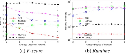
Effect of Average Degree of Diffusion Network

To study the effect of diffusion network’s average degree on algorithm performance, we test the algorithms on five synthetic networks, i.e., LFR6–10, of which the average degrees vary from 2 to 6. We simulate 150 times of dif-fusion processes on each network (i.e.,β = 150). In each simulation,0.15nnodes are randomly selected as the initial infected nodes (i.e.,α= 0.15).

(7)

0.05 0.1 0.15 0.2 0.25 0

0.2 0.4 0.6 0.8 1

Initial Infection Ratio

F−score

(a)F-score

0.05 0.1 0.15 0.2 0.25 10−2

100 102

Runtime (seconds)

S2R NetRate Hyper

MulTree TWIND

(b)Runtime

Figure 3: Effect of initial infection ratio on NetSci

0.05 0.1 0.15 0.2 0.25 0

0.2 0.4 0.6 0.8 1

F−score

S2R NetRate Hyper

MulTree TWIND

(a)F-score

0.05 0.1 0.15 0.2 0.25 100

102 104

Runtime (seconds)

S2R NetRate Hyper

MulTree TWIND

(b)Runtime

Figure 4: Effect of initial infection ratio on DUNF

average degree exceeds 5. Compared with the other tested algorithms, our TWIND algorithm has a reasonably better accuracy performance. (2) The runtimes of NetRate, Hyper, MulTree, S2R and TWIND increase with the growth of av-erage degree, and TWIND shows a significant advantage on efficiency performance over NetRate, Hyper and MulTree.

Effect of Initial Infection Ratio

The ratio of initially infected nodes may affect the number of final infected nodes. To study the effect of initial infection ratio on algorithm performance, we test the algorithms on two real-world networks NetSci and DUNF with different initial infection ratiosα(vary from 0.05 to 0.25). For each initial infection ratio, we simulate 150 times of diffusion processes on each network (i.e.,β= 150).

Figs. 3 & 4 illustrate the F-score and runtime of each al-gorithm on NetSci and DUNF, respectively. From the figures we can observe that (1) a greater initial infection ratio tends to improve the accuracy performance of MulTree, while degrading the accuracy performance of NetRate, Hyper and S2R. TWIND is reasonably insensitive to initial infection ratio and has better accuracy performance. (2) The increase of initial infection ratio has little effect on the runtime of NetRate, Hyper, S2R and TWIND, but results in more runtime for MulTree. Similar results can also be observed on synthetic networks LRF1–10.

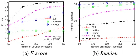
Effect of Amount of Diffusion Processes

The inference of diffusion network is based on the observed diffusion results of diffusion processes. Hence, the amount of diffusion processes may affect the accuracy performance of diffusion network inference. Generally, more diffusion

50 100 150 200 250 0.1

0.2 0.3 0.4 0.5 0.6 0.7

Number of Diffusion Processes

F−score

(a)F-score

50 100 150 200 250 100

101 102 103

Runtime (seconds)

(b)Runtime

Figure 5: Effect of number of diffusion processes on NetSci

50 100 150 200 250 0.1

0.2 0.3 0.4 0.5 0.6 0.7 0.8 0.9

F−score

S2R NetRate Hyper

MulTree TWIND

(a)F-score

50 100 150 200 250 100

102 104

Runtime (seconds)

(b)Runtime

Figure 6: Effect of number of diffusion processes on DUNF

processes will contain more information about diffusion net-work, and help the diffusion network inference algorithms to achieve more accurate inference results. To study the effect of the amount of diffusion processes on algorithm performance, we test the algorithms on two real-world networks NetSci and DUNF with different number β of diffusion processes (β varies from 50 to 250). In each diffusion process, we randomly selected0.15nnodes as the initial infection nodes (α= 0.15).

Figs. 5 & 6 illustrate the F-score and runtime of each algorithm on NetSci and DUNF, respectively. From the figures we can observe that (1) a greater amount of diffusion processes often helps the tested algorithms to achieve more accurate results on diffusion network structure inference. TWIND often has a better accuracy performance compared with the other tested algorithms. (2) To analyze the infection status results observed from more diffusion processes, the tested algorithms often require more runtime. Compared with NetRate, Hyper and MulTree, TWIND shows a signif-icant advantage on efficiency performance. Similar results can also be observed on synthetic networks LRF1–10.

Conclusion

(8)

we have also presented a heuristic pruning method for candidate parent nodes to reduce redundant computation during the identification of the most probable parent nodes. Extensive experiments on both synthetic and real-world networks have been conducted, and the results have verified the effectiveness and efficiency of our approach.

Acknowledgments

This research was supported partly by the NSFC Grants 61502347, 61502504 and 61522208, the Technological In-novation Major Projects of Hubei Province under Grant No. 2017AAA125, Beijing Municipal Science and Tech-nology Projects under Grant No. Z171100005117002, and the Science and Technology Program of Wuhan City under Grant No. 2018010401011288, in which Di’s work was supported in part by the NSERC Canada under the grant CRDPJ 479555 Niu. Wei Lu is the corresponding author.

References

Abrahao, B.; Chierichetti, F.; and Kleinberg, R. 2013. Trace complexity of network inference. InKDD 2013, 491–499.

Amin, K.; Heidari, H.; and Kearns, M. 2014. Learning from contagion(without timestamps). InICML 2014, 1845–1853. Daneshmand, H.; Gomez-Rodriguez, M.; Song, L.; and Sch¨olkopf, B. 2014. Estimating diffusion network structures: Recovery conditions, sample complexity & soft-thresholding algorithm. InICML 2014, 793–801.

Du, N.; Song, L.; Smola, A.; and Yuan, M. 2012. Learning networks of heterogeneous influence. InNIPS 2012, 2780– 2788.

Gomez-Rodriguez, M., and Sch¨olkopf, B. 2012. Submod-ular inference of diffusion networks from multiple trees. In

ICML 2012, 489–496.

Gomez-Rodriguez, M.; Balduzzi, D.; and Sch¨olkopf, B. 2011. Uncovering the temporal dynamics of diffusion networks. InICML 2011, 561–568.

Gomez-Rodriguez, M.; Leskovec, J.; and Krause, A. 2010. Inferring networks of diffusion and influence. InKDD 2010, 1019–1028.

Gomez-Rodriguez, M.; Leskovec, J.; and Sch¨olkopf, B. 2013a. Modeling information propagation with survival theory. InICML 2013, 666–674.

Gomez-Rodriguez, M.; Leskovec, J.; and Sch¨olkopf, B. 2013b. Structure and dynamics of information pathways in online media. InWSDM 2013, 23–32.

Gripon, V., and Rabbat, M. 2013. Reconstructing a graph from path traces. InISIT 2013, 2488–2492.

He, X.; Rekatsinas, T.; Foulds, J.; Getoor, L.; and Liu, Y. 2015. Hawkestopic: A joint model for network inference and topic modeling from text-based cascades. InICML 2015, 871–880.

He, X.; Xu, K.; Kempe, D.; and Liu, Y. 2016. Learning influence functions from incomplete observations. InNIPS 2016, 2065–2073.

Huang, H.; Chiew, K.; Gao, Y.; Q, H.; and Li, Q. 2014. Rare category exploration.Expert Systems with Applications

41(9):4197–4210.

Kalimeris, D.; Singer, Y.; Subbian, K.; and Weinsberg, U. 2018. Learning diffusion using hyperparameters. InICML 2018, 2420–2428.

Lancichinetti, A.; Fortunato, S.; and Radicchi, F. 2008. Benchmark graphs for testing community detection algo-rithms. Physical Review E78(4).

Leskovec, J.; Adamic, L. A.; and Huberman, B. A. 2007. The dynamics of viral marketing.ACM Transactions on the Web1(1):5.

Lokhov, A. 2016. Reconstructing parameters of spreading models from partial observations. In NIPS 2016, 3467– 3475.

Myers, S., and Leskovec, J. 2010. On the convexity of latent social network inference. InNIPS 2010, 1741–1749. Narasimhan, H.; Parkes, D. C.; and Singer, Y. 2015. Learnability of influence in networks. InNIPS 2015, 3186– 3194.

Netrapalli, P., and Sanghavi, S. 2012. Learning the graph of epidemic cascades. InSIGMETRICS 2012, 211–222. Newman, M. E. J. 2006. Finding community structure in networks using the eigenvectors of matrices. Physical Review E74(3):036104.

Pouget-Abadie, J., and Horel, T. 2015. Inferring graphs from cascades: A sparse recovery framework. In ICML 2015, 977–986.

Rong, Y.; Zhu, Q.; and Cheng, H. 2016. A model-free approach to infer the diffusion network from event cascade. InCIKM 2016, 1653–1662.

Sefer, E., and Kingsford, C. 2015. Convex risk minimization to infer networks from probabilistic diffusion data at multiple scales. InICDE 2015, 663–674.

Tang, Y.; Xiao, X.; and Shi, Y. 2014. Influence max-imization: Near-optimal time complexity meets practical efficiency. InSIGMOD 2014, 75–86.

Wallinga, J., and Teunis, P. 2004. Different epidemic curves for severe acute respiratory syndrome reveal similar impacts of control measures. American Journal of Epidemiology

160(6):509–516.

Wang, S.; Hu, X.; Yu, P.; and Li, Z. 2014. MMRate: Inferring multi-aspect diffusion networks with multi-pattern cascades. InKDD 2014, 1246–1255.