R E S E A R C H
Open Access
Regularized minimum class variance extreme
learning machine for language recognition
Jiaming Xu
1,2*, Wei-Qiang Zhang
3, Jia Liu
3and Shanhong Xia
1Abstract
Support vector machines (SVMs) have played an important role in the state-of-the-art language recognition systems. The recently developed extreme learning machine (ELM) tends to have better scalability and achieve similar or much better generalization performance at much faster learning speed than traditional SVM. Inspired by the excellent feature of ELM, in this paper, we propose a novel method called regularized minimum class variance extreme learning machine (RMCVELM) for language recognition. The RMCVELM aims at minimizing empirical risk, structural risk, and the intra-class variance of the training data in the decision space simultaneously. The proposed method, which is
computationally inexpensive compared to SVM, suggests a new classifier for language recognition and is evaluated on the 2009 National Institute of Standards and Technology (NIST) language recognition evaluation (LRE). Experimental results show that the proposed RMCVELM obtains much better performance than SVM. In addition, the RMCVELM can also be applied to the popular i-vector space and get comparable results to the existing scoring methods.
Keywords: Language recognition; Extreme learning machine; Single-hidden layer feedforward neural networks; Support vector machine
1 Introduction
The task of spoken language recognition is to automat-ically determine the identity of the language spoken in a speech sample [1]. It has received increasing attention due to its importance for the enhancement of automatic speech recognition (ASR) [2] and multi-language transla-tion systems [3, 4].
The most popular language recognition techniques can usually be categorized as phonotactic [5–7] and acous-tic approaches [8, 9]. The former method is based upon phone recognizer followed by language models (PRLM), parallel PRLM (PPRLM), and supper vector machines PRLM. The later approach uses shifted-delta-cepstral (SDC) coefficients as a means of incorporating temporal information about the speech into the feature vector.
The introduction of support vector machines (SVMs) into language recognition resulted in significant improve-ment in performance [10]. SVMs have proven to be an effective method and have been widely used for many
*Correspondence: [email protected]
1State Key Laboratory of Transducer Technology, Institute of Electronics, Chinese Academy of Sciences, 100190 Beijing, China
2University of Chinese Academy of Sciences, 100190 Beijing, China Full list of author information is available at the end of the article
years [11]. SVMs perform a nonlinear mapping from an input space to an SVM feature space. The standard opti-mization method is then used to find the solution of max-imizing the separating margin of two different classes in this potentially high-dimensional feature space while min-imizing the training errors. In language recognition, we usually adopt the one-versus-rest tactic to deal with mul-ticlass classification problems when using SVMs, namely, setting data from target language as the positive samples and data from all the other languages as the negative sam-ples. In this way, the amount of training samples between the positive language and negative languages is unbal-anced and sometimes it is even impossible to separate them properly by a linear hyperplane. In addition, the training of SVMs involves a quadratic programming (QP) problem, the computational complexity of SVM training algorithms is usually intensive, which is at least quadratic with respect to the number of training samples.
In recent years, extreme learning machine (ELM) [12, 13] has emerged and attracted the attention from more and more researchers. ELM is a single-hidden layer feedforward network (SLFN) which randomly selects input weights and hidden neuron biases without training.
The output weights are analytically determined by Moore-Penrose generalized inverse. The input weights are the weights of the connections between input neurons and hidden neurons and the output weights are the weights of the connections between hidden neurons and output neurons. ELM overcomes the proposed challenges faced by SVMs. Solving the regularized least square problem in ELM is faster than solving the quadratic program-ming problem in standard SVMs. Recent papers show that predicting accuracy achieved by ELM is comparable with or even higher than that of SVMs [14, 15]. Besides, ELM can learn the training data not only one-by-one but also chunk-by-chunk [16], so it provides a promis-ing method to deal with big data. Moreover, traditional kernel methods can also be applied to ELM [15]. Due to its excellent features, ELM has been successfully used in many areas and there has been increasing research inter-est in it [17–19]. Many researchers have came up with some methods to improve ELM theories, such as ELMs for noisy/missing data [20, 21] and imbalanced data [22]. In [23], minimum class variance extreme learning machine (MCVELM) was proposed for human action recognition and achieved excellent performance. MCVELM borrows the idea from minimum class variance support vector machines (MCVSVM) [24] which is inspired from the optimization of Fisher’s discriminant ratio. The objec-tive of MCVELM is to minimize both the intra-class variance of training data in the decision space and the training errors. However, the MCVELM does not take the structural risk into consideration, so it can lead to the over-fitting problem.
Inspired by its successful application to classification problems, in this paper, we introduce ELM into spoken language recognition, hoping to open up a new research direction for language recognition community. A new method referred to as regularized minimum class variance extreme learning machine (RMCVELM) is proposed and used as classifier for language recognition. Different from MCVELM, the proposed RMCVELM also minimizes the output weight norm directly which can effectively pre-vent the over-fitting problem. Therefore, the proposed RMCVELM can be considered as minimizing empirical risk, structural risk, and the intra-class variance of the training data in the decision space simultaneously. Since RMCVELM is based on structural risk minimization, it can be expected to provide better generalization ability.
To evaluate the effectiveness of the proposed RMCVELM, in this work, two types of acoustic features are used, GMM supervectors (GSVs) [25] and i-vectors [26]. The GSV has been widely used for many years and the i-vector approach, which provides an elegant way to capture the majority of useful variabilities of an utterance, has proven to be one of the most successful methods for language recognition nowadays [27, 28].
The outline of the paper is as follows. In Section 2, we introduce the ELM algorithm briefly. The proposed RMCVELM is described in detail in Section 3. In Section 4, experimental setup is introduced. In Section 5, we demonstrate the potential of the algorithm by applying it to language recognition task. In Section 6, computa-tional complexity is analyzed. Finally, some conclusions are given in Section 7.
2 Overview of extreme learning machine 2.1 Basic extreme learning machine
ELM was first proposed by Huang [12] as an extremely simple and efficient method to train the single-hidden layer feedforward network. He has proven that the SLFN network with randomly chosen input weights and hidden neuron biases can approximate any continuous function to any desirable accuracy [29]. The input weights and hid-den biases need not be tuned after randomly selected, and the output weights are analytically calculated using Moore-Penrose generalized pseudo-inverse.
Let us denote the training data asℵ = {(xi,ti)|xi∈Rd,
i = 1,. . .,N}, wheredis the dimension of training data andN is the number of training data.ti is the label ofxi which is a vector of lengthm,mis the number of classes. If
xibelongs to classj, then all elements oftiare zero except thejth element, which takes the value 1.
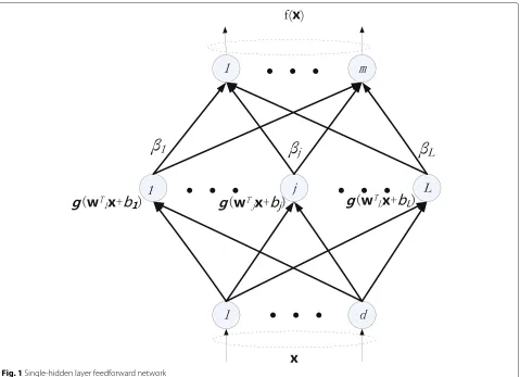
The structure of ELM is shown in Fig. 1.Lis the number of hidden nodes.wjandbjare the input weights and bias of thejth hidden node, respectively. Hidden node param-eterswjandbjremain fixed after randomly generated.βj is the output weights of thejth hidden node. The output of hidden layer with respect to training dataxiish(xi),
h(xi)=
g
wT1xi+b1
. . .g
wTLxi+bL
(1)
where g(wTj xi+ bj) is the activation function of thejth hidden node. Many activation function can be used, such as sigmod, sine, and RBFs. The most widely used is the sigmod function.
g
wTj xi+bj
= 1
1+exp
−wTj xi+bj
(2)
From the perspective of ELM,h(xi)is a feature map which transforms the samplexiinto ELM feature space.
The hidden layer output matrixHis defined as:
H=
⎡ ⎢ ⎣
g wT1x1+b1
. . . g wTLx1+bL
..
. · · · ...
g wT1xN +b1
. . . g wTLxN+bL
⎤ ⎥ ⎦
N×L (3)
Fig. 1Single-hidden layer feedforward network
The target of original ELM is to minimize the training error, namely
minimize:Hβ−T22 (4)
where
β= ⎡ ⎢ ⎣
βT
1
.. .
βT L
⎤ ⎥ ⎦
L×m
T=
⎡ ⎢ ⎣
tT1
.. .
tTN
⎤ ⎥ ⎦
N×m
(5)
The solution of the above linear system is:
β=H†T (6)
The orthogonal projection method can be efficiently used in ELM, namely H† = HTH−1HT if HTH is nonsingular orH†=HT HHT−1ifHHTis nonsingular. During the test stage, a test dataxis scored using the following equation,
f(x)=h(x)β=h(x)(HTH)−1HTT (7)
or
f(x)=h(x)β=h(x)HT
HHT
−1
T (8)
2.2 Regularized extreme learning machine
The basic ELM described previously directly uses the nor-mal equations for the least squares problem, so it can be considered as based on empirical risk minimization and tends to have over-fitting problems. Adding a regulariza-tion term to the error funcregulariza-tion can control over-fitting [30]. Based on this idea, the objective function of regu-larized extreme learning machine (RELM) can be written as,
Minimize:Hβ−T22+ C
2 β
2
2 (9)
where C is the user specified parameter and provides a tradeoff between the training error and the regularization termβ22. Similar to ELM, the solution to RELM can be written as,
β=HTH+CI
−1
HTT (10)
In [13], Huang has discussed the similarities between RELM and SVM and proven that to minimize the norm of the output weightβ2is actually to maximize the
the ELM feature space, which is similar to SVM. This con-clusion is quite important and will be further discussed when introducing the RMCVELM.
3 Regularized minimum class variance extreme learning machine
Based on the previous introduction, in this section, we will describe RMCVELM in detail. We will first introduce the MCVELM and show some of it advantages when deal-ing with classification problems under certain conditions. Then the drawback of this algorithm is illustrated and RMCVELM is proposed to overcome the challenge faced by MCVELM.
3.1 Minimum class variance extreme learning machine
In [23], minimum class variance extreme learning machine (MCVELM) was proposed for human action recognition. MCVELM borrows the idea from minimum class variance support vector machines (MCVSVM) [24] which is inspired from the optimization of Fisher’s dis-criminant ratio. Instead of finding the maximum separat-ing margin, MCVSVM aims at findseparat-ing a hyperplane along which the intra-class variance of the training data is mini-mum. Similar to MCVSVM, the objective of MCVELM is to minimize both the intra-class variance of training data in the decision space and the training errors. The objective function of RMCVELM has the form
Minimize:1 2
N
i=1
ξi2 2+
C
2tr
βTS wβ
Subject to:h(xi)β=tTi −ξTi ,i=1,. . .,N (11) wheretr()is the trace of a matrix andξi=ξi,1,. . .,ξi,m
T
is the training error vector of the moutput nodes with respect to the training samplexi. Swis the within-class scatter matrix of the training samples in the ELM space defined by
Sw= m
k=1
i∈Ck
(h(xi)−mk) (h(xi)−mk)T (12)
whereNkis the number of training samples in the classk andmk = N1k
Nk
i=1h(xi)is the mean vector of classk. So
the termtr
βTS wβ
represents intra-class variance of all the training samples in the decision space. The solution to MCVELM can be written as
β=HTH+CSw −1
HTT (13)
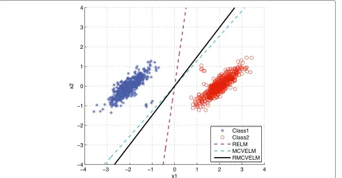
Compared with RELM, MCVELM takes the distribu-tion of all the training data in the ELM feature space into consideration, not only the data near the separating mar-gin. From Fig. 2, we can easily find the difference between RELM and MCVELM. In Fig. 2, some synthetic data are used to simulate samples in the ELM feature space. Two
−4 −3 −2 −1 0 1 2 3 4
−4 −3 −2 −1 0 1 2 3 4
x1
x2
Class1 Class2 RELM MCVELM RMCVELM
classes of Gaussian distribution data are randomly gen-erated and several samples are added near the margin between the two classes. Then RELM and MCVELM are used to classify the data. As shown in Fig. 2, RELM tries to find a maximum separating margin, but this separating hyperplane can not effectively describe the data distri-bution so it loses some information which is helpful to classification. In this case, MCVELM can find a more rational separating hyperplane which is more consistent with the data distribution.
3.2 Regularized minimum class variance extreme learning machine
From previous analysis, we can see that MCVELM, which tries to find a separating hyperplane along which the intra-class variance is minimum can work better than RELM
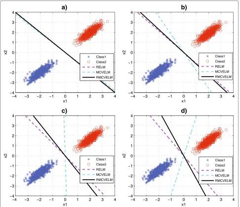
under certain conditions; however, there will be a seri-ous problem when the samples are distributed as shown in Fig. 3. From Fig. 3a–d, the mean of each Gaussian is changed gradually along the x2-axis. Here we denote the mean vector of Class1 as μ1 and the mean vector of Class2 as μ2.μ1 and μ2 in the four sub-figures are shown in Table 1. In this case, it is obvious that the hyper-plane based on MCVELM can not separate the two classes properly. When there are slight changes in the relative position between the two classes, the separating hyper-plane obtained by MCVELM varies greatly, as shown in Fig. 3b–d, it rotates clockwise greatly. Besides minimizing training error, MCVELM always tries to find a separat-ing line along which the intra-class variance is minimum, while the samples near the margin which can provide more important classification information are neglected.
a)
b)
c)
d)
Table 1Mean vectors in Fig. 3
Fig. 3 a b c d
μ1 [−2,−2] [−2,−1.9] [−2,−1.7] [−2,−1.5]
μ2 [2,2] [2,1.9] [2,1.7] [2,1.5]
This objective makes the MCVELM too sensitive to the changes in the relative position between the two classes, even when the changes are not so big. So MCVELM tends to find separating hyperplanes as shown in Fig. 3. In this case, the samples from the two classes tend to overlap if they are projected onto the direction onto which the intra-class variance of training samples is minimum. The RELM, on the contrary, which aims at finding the max-imum separating margin is not so sensitive to the slight position changes. Its separating hyperplane only rotates clockwise slightly. Under this condition, the samples near the margin can provide much more important informa-tion for classificainforma-tion, so RELM can work better than MCVELM. Therefore, the maximum margin term is quite important and should be taken into consideration.
From another point of view, as stated in Section 2.2, regularization termβ22can also be considered as struc-tural risk. According to statistical learning theory, the real prediction risk of learning is consisted of empirical risk and structural risk. A model with good generaliza-tion ability should have the best trade-off between the two risks. However, MCVELM does not take the struc-tural risk into consideration. Therefore MCVELM can not always achieve good generalization performance.
From the previous analysis, we can see that under certain conditions RELM can work quite better than MCVELM and vice versa. Each algorithm has its own advantages and drawbacks and no algorithm can work well under all conditions. However, the differences between the two algorithms also suggest that RELM and MCVELM could be complementary to each other. That means a combination of the two algorithms can provide a more robust classification algorithm. Based on this idea, in this work, we propose the regularized minimum class variance extreme learning machine (RMCVELM) which minimizes the empirical risk, structural risk, and intra-class variance of training data in the decision space simul-taneously. Different from MCVELM, the output weight norm is minimized directly. The objective function of RMCVELM has the form
Minimize:1 2
N
i=1
ξi2 2+
C1
2 β
2 2+
C2
2 tr
βTS wβ
Subject to:h(xi)β=tTi −ξTi ,i=1,. . .,N
(14)
As stated before, β22 is the regularization term which aims at finding maximum separating margin in the ELM space and preventing over-fitting problem and
trβTSwβ
represents intra-class variance of all the train-ing samples in the decision space.
By submitting the constraints into the objective func-tion, we obtain the following equivalent unconstrained optimization problem,
Minimize:1
2 Hβ−T
2 2+
C1
2 β
2 2+
C2
2 tr
βTS wβ
(15)
The gradient of this objective function with respect toβ can be written as,
∇ =HT(Hβ−T)+C1β+C2Swβ (16)
By setting the gradient to zero, we obtain the solution to the RMCVELM,
β=HTH+C1I+C2Sw −1
HTT (17)
During the test stage, a test data x is scored by the following equation,
f(x)=h(x)β (18)
The RMCVELM algorithm is summarized as follows.
Algorithm 1RMCVELM Algorithm
Given hidden node output functiong(wjx+bj)and hidden node numberL:
1: Randomly generate hidden nodes parameters (wj,bj),j=1,. . .,L.
2: Calculate the hidden output matrixH.
3: Calculate the within-class scatter matrix Sw in the ELM space.
4: Calculate the output matrixβusing Eq. (17). 5: calculate score for a test dataxusing Eq. (18).
We should note that RMCVELM can be considered as a unified mode for basic ELM, RELM, and MCVELM. WhenC1 = C2 = 0, RMCVELM is equivalent to basic
ELM. IfC1 = 0 RMCVELM is equivalent to MCVELM
and ifC2 = 0 RMCVELM is equivalent to RELM. From
but also use the samples near the margin which play an important role in classification. So RMCVELM can work well in these two cases.
4 Experimental setup
4.1 Training, development and evaluation data
The experimental setup for this work is based on the NIST 2009 Language Recognition Evaluation (LRE) [31]. The 2009 LRE consisted of 23 linguistic classes. The 23 linguistic classes are Amharic, Bosnian, Cantonese, Creole, Croatian, Dari, American, English--Indian, Farsi, French, Georgian, Hausa, Hindi, Korean, Mandarin, Pashto, Portuguese, Russian, Spanish, Turkish, Ukrainian, Urdu, and Vietnamese. Both conversational telephone speech utterances (CTS) and narrow band telephone segments from Voice of America broadcasts (VOA) are used as data sources for the 23 linguistic classes.
The training data consists of both CTS and VOA data. The CTS samples come from previous NIST LRE (2007) and the CallFriend, CallHome, OGI-22 collections. The VOA data consist of narrow band segments from VOA broadcasts. We totally have about 30,000 samples for the whole training set.
The calibration back-end described in Section 4.3 was trained on development dataset, which comprises data from the dataset provided by NIST for the 2003, 2005, and 2007 LRE and VOA. Only data of the 23 target languages are used. This set has about 10,000 samples.
The evaluation set consists of all the data from the NIST 2009 LRE. Experiments are performed on the 23 languages closed-set task. The criterion for evaluation is pooled equal error rate (EER) and average cost Cavg
defined by NIST.
4.2 Feature extraction
For feature extraction, we first extract 13-dimensional MFCC features and the cepstral features are processed with RASTA filtering. Then SDCC features [8] are used with a 7-1-3-7 parameterization.
A language and gender independent UBM [32] is trained using all of the training data with eight iterations of EM adapting all parameters-means, mixture weights, and diagonal covariances. The number of mixture compo-nents is 512.
After that, two different kinds of features are extracted for each utterance, namely GMM Supervectors (GSVs) [25] and i-vectors [26].
For the GSV extraction, a GMM is trained for each utterance, only means are adapted for GMM MAP train-ing. The GSV for a given utterance is the stacked mean supervector which is normalized as follows,
mi=
λi−1/2
i mi (19)
whereλi, i andmi are the mixture weight, covariance and mean of theith GMM component. A 28,672 dimen-sional GSV is extracted for each utterance. The GSVs are then compensated using Nuisance Attribute Projection (NAP) [33].
The i-vectors framework has become very popular in speaker and language recognition. The main idea is that the GMM supervector (vector created by stacking all mean vectors from the GMM) for a given utterance can be modeled as follows,
M=m+Tw (20)
wheremis the language- and channel-independent mean supervector (which can be taken to be the UBM supervec-tor),Tis a rectangular matrix of low rank and the i-vector
wis a random vector having a standard normal distribu-tion. For a given utterance, we use the standard method to extract the i-vector as described in [26]. The dimension of each i-vector is 400.
4.3 Calibration back-end
The calibration back-end [34] uses the scores from the classifiers described above rather than the GSVs or the i-vectors. It is trained on the separate development dataset described in Section 4.1 to obtain well-calibrated scores. Here, we use the MMI back-end [35] for calibration.
5 Experimental result 5.1 GSV systems
In order to evaluate the effectiveness of the proposed RMCVELM algorithm on language recognition perfor-mance, we first compare its performance with that of SVM, MCVELM, and RELM on the GSV features.
In our RMCVELM system, the input weightwi is ran-domly generated between−0.5 and+0.5, and bi is ran-domly generated between 0 and +1. The number of hidden node is 20,000. Here we use cross-validation tech-nique on the training data to determine the parametersC1
andC2. The training data is partitioned into four groups.
Then three of the groups are used to train a set of mod-els that are then evaluated on the remaining group. This procedure is then repeated for all four possible choices for the groups, and the four performance scores are then aver-aged. According to this cross-validation technique, the optimal parameters are set to beC1=2000 andC2=5.
In the SVM system, we use the proposed one-versus-rest strategy which is the standard method widely used for language recognition. The C value for SVM is set to be 0.8, it is tuned by the cross-validation technique as stated in the RMCVELM system.
In the MCVELM system,C1is set to be 0 andC2=1.5
which is achieved by the cross-validation technique stated above. Similarly, in the RELM system,C2is set to be 0 and
We also train a standard neural network (NN) with the same architecture as the ELM for comparison. The hid-den node number is 120 and learning rate is 0.05. Besides, dropout method is used, the dropout fraction is 0.8. In addition, the weight penalty term based on L2 norm is
also taken into consideration. The coefficient of the weight penalty term is 0.005. We find that the dropout method and the weight penalty term must be used or there will be a serious over-fitting problem. All the above parameters are set by the cross-validation technique stated above.
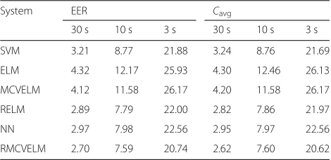
Results for the various systems on GSV features are shown in Table 2.
First, we can easily note that the proposed RMCVELM outperforms SVM at all the three different durations. Especially, RMCVELM can greatly enhance the perfor-mance at the 30-s duration, obtaining at most 15 % (EER) and 19 % (Cavg) relative improvement compared
with SVM, respectively. In addition, RMCVELM works quite better than MCVELM and RELM, which verifies our theory. RMCVELM is more robust compared with MCVELM and RELM.
We should also note that the NN is better than the basic ELM which has no regularization term and com-parable to the RELM. This is because the regularization term plays an important role in preventing the over-fitting problem. However, the NN does not achieve better per-formance than RELM, one reasonable explanation is that the NN tends to have the local minima problem. The advantages of ELM compared to NN has been discussed in detail in [12] which shows that ELM can achieve better performance than NN in many applications.
5.2 I-vector systems
For the i-vector inputs, all the i-vectors are centered on the origin and then linear discriminant analysis(LDA) is used to reduce the dimension. Since we have 23 target lan-guages, each i-vector is reduced to 22 dimensions. Each i-vector is unit normalized after LDA, here we use li to denote the normalized i-vector after LDA for a given utterancei.
Table 2Comparison of EERs (%) andCavgfor different training
methods based on GSV at different durations for the 23 proposed languages of LRE09
System EER Cavg
30 s 10 s 3 s 30 s 10 s 3 s
SVM 3.21 8.77 21.88 3.24 8.76 21.69
ELM 4.32 12.17 25.93 4.30 12.46 26.13
MCVELM 4.12 11.58 26.17 4.20 11.58 26.17
RELM 2.89 7.79 22.00 2.82 7.86 21.97
NN 2.97 7.98 22.56 2.95 7.97 22.56
RMCVELM 2.70 7.59 20.74 2.62 7.60 20.62
We first apply the cosine distance scoring (CDS) to score the i-vector, which has been widely used in language recognition [36].
scorel=mTl ∗ltest (21)
wheremlis the model of languagel,
ml = Nl
i=1li
Nl
i=1li2
(22)
In addition, a widely used generative model called Gaus-sian back-end (GB) [28] is also used for comparison. In this case, i-vector distribution for each language is mod-eled by a Gaussian distribution, here a full covariance matrix is shared across all languages. During the test stage, each i-vectorltestis scored as:
scorel = − 1 2l
T
test−1l
test+lTtest−1μl−
1 2μ
T
l −1μl+const
(23)
whereμl is the mean vector for languagelandis the covariance matrix.
Then SVM, NN, and RMCVELM are applied to the i-vector. The C value for SVM is 1.2. For the NN, the hidden node number is 80, and learning rate is 0.01. The dropout fraction is 0.45, and the coefficient of theL2norm weight
penalty term is 0.006. For the RMCVELE system, The number of hidden node is 3000 (experiments show that there is no significant improvement when the number of hidden node increases), and C1 = 2100,C2 = 3. All
the parameters are determined as that in the GSV feature space.
The performance of the different methods are shown in Table 3. The results demonstrate that RMCVELM can achieve comparable performance to the widely used CDS and GB method. So it can also be successfully applied to the i-vector space.
In addition, we can easily note that the CDS and GB which are used as baselines can achieve similar perfor-mance. Here we think that the CDS can approximate the GB. Since all i-vectors are unit vectors and centered on the origin, the mean of the Gaussian distribution for each
Table 3Comparison of EERs (%) andCavgfor different training
methods based on i-vector at different durations for the 23 proposed languages of LRE09
System EER Cavg
30 s 10 s 3 s 30 s 10 s 3 s
CDS 2.63 6.72 20.22 2.59 6.80 20.36
GB 2.65 6.77 19.90 2.60 6.86 20.02
SVM 2.70 6.78 19.92 2.62 6.97 19.80
NN 2.95 7.87 21.32 2.93 7.92 21.54
language is approximately on the circle centered on the origin. The CDS averages i-vectors for a language, the model can roughly be regarded as a vector pointing from the origin to the mean of the Gaussian distribution for this language, so the separating margin between two classes is a linear hyperplane which is through the origin and equally divides the angle formed by the models of the two classes. The GB uses a shared covariance matrix, so the separating margin between two classes is also a linear hyperplane. If the covariance matrix is a diagonal matrix and the diagonal elements are the same, the GB hyper-plane also will be through the origin and will be quite close to the CDS hyperplane. In this experiment, we find that the main diagonal elements of the full covariance matrix are much larger than other elements, so the full covariance matrix is close to a diagonal matrix. In addition, the main diagonal elements are close to each other. In this case, we can assume that the CDS is almost equivalent to the GB. So the two methods can achieve similar performance.
Besides, the NN can not get good performance as it is often very sensitive to many parameters, such as learn-ing rate and dropout fraction, and tends to have the local minima problem.
5.3 Discussion
The experimental results show that in most cases, RMCVELM can achieve better performance than SVM. Compared with SVM, RMCVELM has some potential advantages.
In [13], the differences and similarities between SVM and ELM has been discussed. ELM and SVM have sim-ilar optimization formula. However, in SVM optimal
Lagrange multipliers αi are found from the hyperplane N
i=1αiti = 0, so SVM often obtains a suboptimal optimization. Different from SVM, ELM does not need to satisfy this condition, so ELM has milder optimiza-tion constraints and can find αi from the entire space. RMCVELM, which is an extension of ELM, naturally inherits this good feature.
In addition, RMCVELM can be considered as a uni-fied mode for ELM, regularized ELM, and MCVELM. It considers the training error, generalization ability, and dis-tribution of all the training data in the ELM space simulta-neously. By adjusting parametersC1andC2, RMCVELM
can learn much better even when the data distribution varies greatly. So it has the potential to deal with more complicated data. From this point of view, RMCVELM is more robust.
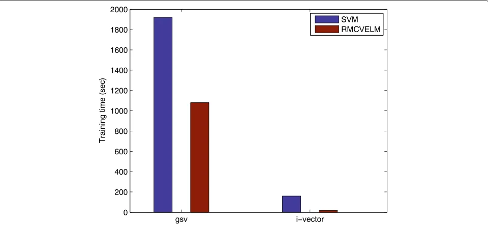
6 Computational complexity
In this section, the computational complexity is compared between SVM and RMCVELM. Training time for the two algorithms are shown in Fig. 4. We can note that the pro-posed RMCVELM is much faster than traditional SVM. The main computational cost for SVM comes from a QP problem, which is at least quadratic with respect to the number of training data. So the computational complex-ity of SVM is usually intensive when dealing with large problems. However, RMCVELM gets a solution based on Eq. (17), where the size of(HTH+C1I+C2Sw)isL∗L. In most applications, the number of hidden nodeLis much smaller than the number of training data:L << N. So RMCVELM can greatly reduce the training time.
7 Conclusions
In this paper, we proposed a novel algorithm regular-ized minimum class variance extreme learning machine for language recognition. The RMCVELM aims at min-imizing empirical risk, structural risk, and the intraclass variance of the training data in the decision space simul-taneously. The proposed method improves the perfor-mance for language recognition and can learn at a much faster speed compared with traditional SVM. In addi-tion, RMCVELM can also be applied to i-vector space and achieves an equivalent performance compared with the CDS and GB method. To our best knowledge, this is the first time such an approach is applied to language recognition.
Competing interests
The authors declare that they have no competing interests.
Acknowledgements
This work is supported by National Natural Science Foundation of China (Project 61370034, Project 61273268 and Project 61005019).
Author details
1State Key Laboratory of Transducer Technology, Institute of Electronics,
Chinese Academy of Sciences, 100190 Beijing, China.2University of Chinese Academy of Sciences, 100190 Beijing, China.3National Laboratory for Information Science and Technology, Department of Electronic Engineering, Tsinghua University, 100084 Beijing, China.
Received: 25 November 2014 Accepted: 3 August 2015
References
1. H Li, B Ma, KA Lee, Spoken language recognition: from fundamentals to practice. Proc. IEEE.101(5), 1136–1159 (2013)
2. F Biadsy, Automatic dialect and accent recognition and its application to speech recognition, PhD thesis, Columbia University (2011)
3. MA Zissman, KM Berkling, Automatic language identification. Speech Comm.35(1), 115–124 (2001)
4. YK Muthusamy, E Barnard, RA Cole, Reviewing automatic language identification. Signal Proc. Mag. IEEE.11(4), 33–41 (1994)
5. MA Zissman, Comparison of four approaches to automatic language identification of telephone speech. IEEE Transactions on Speech and Audio Processing.4(1), 31 (1996)
6. WM Campbell, FS Richardson, DA Reynolds, inICASSP (4). Language recognition with word lattices and support vector machines (IEEE, Honolulu, USA, 2007), pp. 989–992
7. W-Q Zhang, W-W Liu, Z-Y Li, Y-Z Shi, J Liu, Spoken language recognition based on gap-weighted subsequence kernels. Speech Communication. 60, 1–12 (2014)
8. PA Torres-Carrasquillo, E Singer, MA Kohler, RJ Greene, DA Reynolds, JR Deller Jr, inINTERSPEECH. Approaches to language identification using gaussian mixture models and shifted delta cepstral features (ISCA, Denver, USA, 2002)
9. W-Q Zhang, L He, Y Deng, J Liu, MT Johnson, Time-frequency cepstral features and heteroscedastic linear discriminant analysis for language recognition. IEEE Trans. Audio, Speech, and Lang. Process.19(2), 266–276 (2011)
10. WM Campbell, E Singer, PA Torres-Carrasquillo, DA Reynolds, in ODYSSEY04-The Speaker and Language Recognition Workshop. Language recognition with support vector machines (ISCA, Toledo, Spain, 2004) 11. WM Campbell, JP Campbell, DA Reynolds, E Singer, PA
Torres-Carrasquillo, Support vector machines for speaker and language recognition. Comput. Speech & Lang.20(2), 210–229 (2006)
12. G-B Huang, Q-Y Zhu, C-K Siew, inNeural Networks, 2004. Proceedings. 2004 IEEE International Joint Conference On. Extreme learning machine: a new
learning scheme of feedforward neural networks, vol. 2 (IEEE, Budapest, Hungary, 2004), pp. 985–990
13. G-B Huang, DH Wang, Y Lan, Extreme learning machines: a survey. Int. J. Mach. Mach. Learn. Cybern.2(2), 107–122 (2011)
14. G-B Huang, Q-Y Zhu, C-K Siew, Extreme learning machine: theory and applications. Neurocomputing.70(1), 489–501 (2006)
15. G-B Huang, H Zhou, X Ding, R Zhang, Extreme learning machine for regression and multiclass classification. Systems, Man, and Cybernetics, Part B: Cybernetics, IEEE Transactions on.42(2), 513–529 (2012) 16. N-Y Liang, G-B Huang, P Saratchandran, N Sundararajan, A fast and
accurate online sequential learning algorithm for feedforward networks. Neural Netw. IEEE Trans.17(6), 1411–1423 (2006)
17. J Xu, H Zhou, G-B Huang, inInformation Fusion (FUSION), 2012 15th International Conference On. Extreme learning machine based fast object recognition (IEEE, Singapore, 2012), pp. 1490–1496
18. MM Sole, M Tsoeu, inAFRICON, 2011. Sign language recognition using the extreme learning machine (IEEE, Livingstone, Zambia, 2011), pp. 1–6 19. S Suresh, V Babu, N Sundararajan, inControl, Automation, Robotics and
Vision, 2006. ICARCV’06. 9th International Conference On. Image quality measurement using sparse extreme learning machine classifier (IEEE, Singapore, 2006), pp. 1–6
20. P Horata, S Chiewchanwattana, K Sunat, Robust extreme learning machine. Neurocomputing.102, 31–44 (2013)
21. Q Yu, Y Miche, E Eirola, M Van Heeswijk, E Séverin, A Lendasse, Regularized extreme learning machine for regression with missing data.
Neurocomputing.102, 45–51 (2013)
22. W Zong, G-B Huang, Y Chen, Weighted extreme learning machine for imbalance learning. Neurocomputing.101, 229–242 (2013) 23. A Iosifidis, A Tefas, I Pitas, Minimum class variance extreme learning
machine for human action recognition (2013)
24. S Zafeiriou, A Tefas, I Pitas, Minimum class variance support vector machines. Image Process. IEEE Trans.16(10), 2551–2564 (2007) 25. WM Campbell, DE Sturim, DA Reynolds, Support vector machines using
gmm supervectors for speaker verification. Signal Proc. Lett. IEEE.13(5), 308–311 (2006)
26. N Dehak, P Kenny, R Dehak, P Dumouchel, P Ouellet, Front-end factor analysis for speaker verification. Audio, Speech, and Lang. Process, IEEE Trans.19(4), 788–798 (2011)
27. N Dehak, PA Torres-Carrasquillo, D Reynolds, R Dehak, inINTERSPEECH 2011. Language Recognition via I-Vectors and Dimensionality Reduction (ISCA, Florence, Italy, 2011), pp. 857–860
28. D Martınez, O Plchot, L Burget, O Glembek, P Matejka, inProceedings of Interspeech. Language recognition in ivectors space (Firenze, Italy, 2011), pp. 861–864
29. G-B Huang, Learning capability and storage capacity of two-hidden-layer feedforward networks. Neural Networks, IEEE Transactions on.14(2), 274–281 (2003)
30. CM Bishop,Pattern Recognition and Machine Learning, vol. 1. (Springer, New York, 2006)
31. AF Martin, CS Greenberg, inOdyssey. The 2009 nist language recognition evaluation (ISCA, Brno, Czech, 2010), p. 30
32. DA Reynolds, TF Quatieri, RB Dunn, Speaker verification using adapted gaussian mixture models. Digital signal processing.10(1), 19–41 (2000) 33. WM Campbell, DE Sturim, DA Reynolds, A Solomonoff, inAcoustics,
Speech and Signal Processing, 2006. ICASSP 2006 Proceedings. 2006 IEEE International Conference On. Svm based speaker verification using a gmm supervector kernel and nap variability compensation, vol. 1 (IEEE, Toulouse, France, 2006)
34. M Penagarikano, A Varona, M Diez, LJ Rodriguez-Fuentes, G Bordel, in INTERSPEECH. Study of different backends in a state-of-the-art language recognition system, (2012)
35. W ZHANG, T HOU, J LIU, Discriminative score fusion for language identification. Chin. J. Electron.19(1), 124–128 (2010)