R E S E A R C H
Open Access
Accuracy analysis of gradient
reconstruction on isotropic unstructured
meshes and its effects on inviscid flow
simulation
Nianhua Wang
1,2*, Ming Li
2, Rong Ma
2and Laiping Zhang
1,2* Correspondence:nianhuawong@ 126.com
1State Key Laboratory of
Aerodynamics, China Aerodynamics Research and Development Center, Mianyang 621000, China
2Computational Aerodynamics
Institute, China Aerodynamics Research and Development Center, Mianyang 621000, China
Abstract
The accuracy of gradient reconstruction methods on unstructured meshes is analyzed both mathematically and numerically. Mathematical derivations reveal that, for gradient reconstruction based on the Green-Gauss theorem (the GG methods), if the summation of first-and-lower-order terms does not counterbalance in the discretized integral process, which rarely occurs, second-order accurate approximation of face midpoint value is necessary to produce at least first-order accurate gradient. However, gradient reconstruction based on the least-squares approach (the LSQ methods) is at least first-order on arbitrary unstructured grids. Verifications are performed on typical isotropic grid stencils by analyzing the relationship between the discretization error of gradient reconstruction and the discretization error of the face midpoint value approximation of a given analytic function. Meanwhile, the numerical accuracy of gradient reconstruction methods is examined with grid convergence study on typical isotropic grids. Results verify the phenomenon of accuracy degradation for the GG methods when the face midpoint value condition is not satisfied. The LSQ methods are proved to be at least first-order on all tested isotropic grids. To study gradient accuracy effects on inviscid flow simulation, solution errors are quantified using the Method of Manufactured Solutions (MMS) which was validated before adoption by comparing with an exact solution case, i.e., the 2-dimensional (2D) inviscid isentropic vortex. Numerical results demonstrate that the order of accuracy (OOA) of gradient reconstruction is crucial in determining the OOA of numerical solutions. Solution accuracy deteriorates seriously if gradient reconstruction does not reach first-order.
Keywords:Finite volume discretization, Unstructured grids, Gradient reconstruction,
Accuracy analysis, The method of manufactured solutions, Grid convergence study
1 Introduction
In the last several decades, research and applications of unstructured grids in Compu-tational Fluid Dynamics (CFD) numerical simulations had drawn much attention. Unstructured grids offer great flexibility in the treatment of complex geometries, and solution dependent grid adaptivity on unstructured grids can be easily implemented. Despite its advantages, unstructured grids also meet some challenges in improving computational efficiency and obtaining accurate unstructured finite-volume (FV)
discretization schemes. Nowadays, nominally second-order accurate unstructured FV schemes are widely applied in industrial CFD applications. However, the actual numerical accuracy of unstructured FV schemes had long been a hot topic for CFD researchers.
Pioneering work had been done on mathematical and numerical accuracy study of cell-vertex schemes due to Jameson et al. [1] and Ni [2]. Relationship between the con-vergence of truncation error and concon-vergence of discretization error had been studied and clarified that the solution error could be second-order even though the local trun-cation error is first order [3, 4]. Preliminary investigation on the influence of mesh
types on solution accuracy had also been conducted [5] which proved that triangular
schemes can perform as well as quadrilateral schemes under appropriate conditions.
Ever since Barth and Jespersen [6] proposed the limited form of piecewise linear
reconstruction, the upwind schemes based on gradient reconstruction became perhaps the most popular unstructured second-order FV schemes. For these upwind schemes, the first-order accurate gradient is necessary to achieve second-order accurate discretization. The accuracy of gradient reconstruction and gradient accuracy effects on the accuracy of FV schemes became key factors in analyzing the accuracy of FV numerical solution.
Generally, there are mainly two types of gradient reconstruction methods which can be readily implemented on unstructured second-order FV discretization of inviscid and viscous fluxes. One is the gradient reconstruction based on the Green-Gauss theorem (the GG methods); the other is based on the least-squares approach (the LSQ methods). Performances of these two types of reconstruction techniques on unstruc-tured meshes are affected by a number of factors, such as mesh type, mesh quality, mesh regularity, formulation, etc.
On one hand, the comparison of these two types of gradient reconstruction methods was illustrated in earlier papers [7–10]. Valuable experiences were acquired such as these two types of methods produce similar results on regular quadrilateral and
tri-angular meshes [7]; the GG method with either simple averaging or inverse distance
weighted face averaging is inconsistent on irregular grids and fails to achieve the first-order accuracy and thus should not be preferred [8]; the LSQ methods are at least
first-order accurate on arbitrary meshes [9], but accuracy deterioration occurs on highly
stretched grids in the presence of surface curvature [10]. However, despite former
analyses and comparisons, no definitive “best” gradient reconstruction method has
emerged [8] and the fundamental reason for the accuracy degradation was not revealed comprehensively.
Meanwhile, preliminary but successful attempts in creating accurate and robust re-construction of the gradient and eventually improving solution accuracy had been made [8,17].
The focus of this study is analyzing gradient reconstruction methods both mathemat-ically and numermathemat-ically for cell-centered FV schemes, evaluating the gradient effects on solution accuracy of inviscid flow simulations. Cell-vertex schemes, while differing from cell-centered schemes in formulation details, can be analyzed in the same fashion; and they have been considered in previous works [12,13,15]. In this paper, the conditions to ensure at least first-order accurate gradient reconstruction are derived mathematic-ally. Then, verifications are performed on typical isotropic grid stencils by analyzing the relationship between discretization error of gradient reconstruction and discretization error of the face midpoint value approximation of a given analytic function. Numerical accuracy of gradient reconstruction is examined with grid convergence study on typical isotropic grids such as quadrilateral grids, triangular grids, perturbed grids, skewed grids and grids over a cylinder with curve boundary. Since previous studies reported that poor gradient reconstruction accuracy does not necessarily imply large discretization error [13], solution errors have to be quantified to determine the impact of gradient accuracy. Quantification of solution errors require an exact solution and
will be accomplished using the Method of Manufactured Solutions (MMS) [18]. Before
the MMS method was adopted, validation of the method was performed by comparing results with an exact solution case, the 2D inviscid isentropic vortex. Grid convergence studies are carried out to determine the order of accuracy and the absolute magnitude of solution errors. Traditional mesh refinement instead of downscaling tests [19–22] is employed for grid convergence study since consistent refinement is easily carried out on currently considered isotropic grids. All the schemes are implemented within a second-order cell-centered finite volume CFD solver, HyperFLOW [23,24].
This paper is organized as follows: in section II, we briefly introduce the second-order FV discretization schemes. A comprehensive description and mathematical analysis of gradient reconstruction methods are followed in section III. Mathematical gradient accuracy analyses are confirmed numerically in section IV. Next, we present principles of the method of manufactured solutions in section V and validate this method with an exact solution case. Finally, in section VI, gradient accuracy effects on solution accuracy of inviscid flows are investigated with a Euler manufactured solution.
2 Finite volume discretization schemes
In this paper, the discretization of the conservation law is implemented in an integral form [25]:
∂
∂t
Z
Ω
WdΩþ ∮
∂ΩðFc−FvÞdS¼ Z
Ω
QdΩ ð1Þ
2.1 Spatial discretization
The convective flux is discretized with the well-known Roe’s flux-difference splitting scheme [26] as follows:
Fc
ð Þij¼
1
2 FcðWRÞ þFcðWLÞ−ΑRoe ðWR−WLÞ
ð2Þ
where (Fc)ijis the convective flux through the interface of the neighboring control
vol-umeiand j,Fc(WL) andFc(WR) are convective fluxes evaluated with the face left state
WL and the face right state WR, respectively. The way to obtain face left and right states is called ‘solution reconstruction’ which will be discussed below. jΑRoej denotes
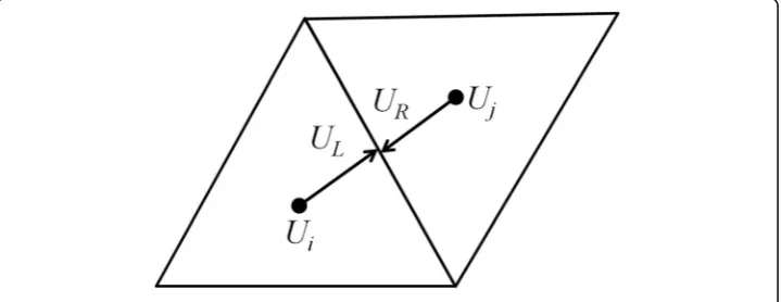
the so-called Roe’s averaged matrix which is identical to the convective flux Jacobian. Anyway, other Riemann solvers for the convective flux can be adopted here, such as Lax-Friedrichs, Steger-Warming, van Leer, HLLC, AUSM series schemes, and so on. No matter which Riemann solver is adopted to calculate the convective flux, the face states on the left and right sides of an interface, the primitive variables UL and URin most cases (as shown in Fig. 1), should be reconstructed firstly. For simplicity, we will denote any one of the primitive variables asUin the following context.
2.2 Solution reconstruction
Roe’s flux-difference splitting scheme, as well as other Riemann solvers, requires flow states to be reconstructed on the left and the right sides of an interface of neighboring control volumes, as sketched in Fig.1.
If we assume that the solution is constant in each cell, a constant reconstruction is obtained which leads to first-order spatial discretization.
UL¼Ui
UR¼Uj ð3Þ
whereULand URare primitive variables at the left and right sides of a control volume
interface. A second-order spatial discretization can be obtained by assuming a linear distribution of flow variables in each cell. With this assumption, the left and the right states are reconstructed through a piecewise linear interpolation as Eq. (4) [6]. Since low speed flows without discontinuity (such as shock wave) are currently studied, no limiter function is considered here.
UL¼Uiþð∇UÞirL
UR¼Ujþð∇UÞjrR ð4Þ
where (∇U)i is the gradient at cell centeri, andrL represents the vector from the left
cell center of i to the face midpoint, and rR represents the vector from the right cell center ofjto the face midpoint.
At least first-order accurate gradient reconstruction is often required in Eq. (4) to achieve second-order accurate spatial discretization. Generally, there are mainly two types of gradient reconstruction methods which can be readily implemented in un-structured second-order finite volume discretization. One is the gradient reconstruction based on the Green-Gauss theorem (the GG methods); the other is based on the least-squares approach (the LSQ methods). These two types of methods are introduced and analyzed in the following section.
3 Gradient reconstruction methods
3.1 Green-gauss theorem based gradient reconstruction
The first type of gradient reconstruction methods is based on the Green-Gauss theorem expressed in Eq. (5).
Z
V
∇UdV ¼ ∮
∂VUndS ð5Þ
where U stands for any one of the primitive variables or any scalar variable, n is the surface unit normal vector. Firstly, we would like to derive the discretized form of Eq. (5).
With the linear distribution assumption of flow variables in each cell, the gradient will be constant within cells; we simplify the left-hand side of Eq. (5) as follows:
Z V ∇UdV 0 @ 1 A i
¼ð∇UÞiVi ð6Þ
where Vi is the volume of the control volume, (∇U)i is the gradient at cell center i.
Combining Eq. (5) with Eq. (6), and introducing the Taylor-series expansion, we derive the discretized gradient of cellias follows:
∇U ð Þi¼ 1
Vi ∂∮VUndS
i
¼ 1 Vi
XNF
j¼1 Z
∂Vj
Uijþ∂∂U xij x−xij
þ∂∂U yij y−yij
þ∂∂U z ij z−zij
nijdS 0 B @ 1 C A ¼ 1 Vi
XNF
j¼1
UijnijΔSijþ
1
Vi
XNF
j¼1 Z
∂Vj ∂U
∂xij x−xij
þ∂U
∂yij y−yij
þ∂U
∂zij z−zij
nijdS
0 B @ 1 C A ð7Þ
in which NFis the number of faces of the control volume, nijΔSijis the area vector of
facejof celli.
Besides, Uijis the value at any point on facejup to now, if we introduce the midpoint quadrature which requires Uijto be the value at the midpoint (centroid) of face j, we obtain:
∇U ð Þi¼ 1
Vi
XNF
j¼1
UijnijΔSij ð8Þ
Here, we would like to emphasize in Eq. (8) that Uij is the value at the midpoint of face j, and at the current stage, the gradient of cell iis represented exactly by Eq. (8) under the linear distribution assumption. Examining Eq. (8) more carefully, we found that potential errors of gradient reconstruction by Eq. (8) can only be introduced by the approximation of face midpoint valueUij.
How does the face midpoint value approximation influence the gradient accuracy? This question is answered by the following mathematical analysis. These derivations focus on the order of magnitude of gradient reconstruction error and face midpoint approximation error.
To find the necessary condition to obtain first-order gradient reconstruction of celli, we need:
∇U
ð Þi numerical ¼ 1 Vi
XNF
j¼1
UijnijΔSij¼ð∇UÞi exactþO hð Þ ð9Þ
where O(h) is the order of magnitude of the mesh size. As mentioned earlier, the only contributor to gradient error is the approximation of face midpoint value. Here we as-sume the face midpoint value approximation to be expressed as follows:
Uij¼Uij^ þaijþbijO hð Þ þcijO h2 ð10Þ
where Uij^ is the exact value at the face midpoint, aij, bij, cij are constant coefficients.
Substituting Eq. (10) into Eq. (9), we obtain:
∇U
ð Þi numerical¼ 1 Vi
XNF
j¼1
^
UijþaijþbijO hð Þ þcijO h2
nijΔSij
¼ 1
Vi XNF
j¼1 ^
UijnijΔSijþ
1 Vi
XNF
j¼1
aijþbijO hð Þ
nijΔSijþ
1 Vi
XNF
j¼1
cijO h2
nijΔSij
ð11Þ
ifPNF
j¼1ðaijþbijOðhÞÞnijΔSij≠0, and
PNF
j¼1ðcijOðh2ÞÞnijΔSij≠0, we have:
∇U
ð Þi numerical¼ð∇UÞi exactþ
aijOð Þ þ1 bijO hð Þ
O h2 O h3 þcij
O h2 O h2 O h3 ¼ð∇UÞi exactþaijO h−
1
þbijOð Þ þ1 cijO hð Þ
ð12Þ
On one hand, we notice that when PNF
j¼1ðaijþbijOðhÞÞnijΔSij¼0 , in other words, the summation (integral) of first-and-lower-order terms in the approximation of face midpoint value counterbalances each other, gradient reconstruction achieves at least first-order accuracy.
Consequently, if no counterbalance occurs for the first-and-lower-order terms, second-order accurate approximation of face midpoint value is necessary to achieve at least first-order gradient reconstruction.
As a supplement, we also prove that second-order accurate approximation of face midpoint value is sufficient to produce first-order accurate gradient.
Assuming that the second-order accurate approximation of the face midpoint value can be written as:
Uij¼Uij^ þO h2 ð13Þ
Substituting Eq. (13) into Eq. (8), we get:
∇U
ð Þi numerical¼ 1 Vi
XNF
j¼1
^
UijþO h2
nijΔSij
¼ 1 Vi
XNF
j¼1
^
UijnijΔSijþ 1 Vi
XNF
j¼1
O h2
nijΔSij
¼ð∇UÞi exactþO h
2
O h2 O h3 ¼ð∇UÞi exactþO hð Þ
ð14Þ
Therefore, in terms of GG gradient reconstruction methods, we conclude that when the summation of first-and-lower-order terms in the integral process does not counter-balance each other, second-order accurate approximation of face midpoint value is the
necessary and sufficient condition for at least first-order accurate gradient
reconstruction.
According to the approach for face midpoint value approximation, the GG methods can be categorized into:
(a) cell-based GG methods (GG-Cell), using the simple average value of face neighboring cells as face midpoint value;
(b) nodal-based GG methods (GG-Node), using the simple average value of node surrounding cells as face nodal value;
(c) GG methods based on least-squares face interpolation (GG-LSQ), using LSQ interpolation to calculate face midpoint value;
(d) GG methods based on weighted tri-linear face interpolation (GG-WTLI), using weighted tri-linear interpolation to calculate face midpoint value.
Readers may refer toAppendix 1for details. Of course, other approaches [11–13,27] can be adopted which are not included in this paper.
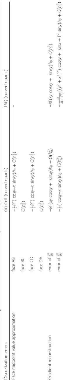
Whether these methods guarantee second-order face midpoint value approximation on arbitrary grids is essential in determining the order of accuracy of gradient recon-struction. Here we tabulate the properties in Table 1 and their verifications are left in later sections.
3.2 Least-squares approach based gradient reconstruction
Uj¼Uiþð∇UÞirijþh:o:t: ð15Þ
whereUiis the variable at the center of celli, andrijis the vector from cell centerito
cell centerj. If second-and-higher-order terms are neglected, Eq. (15) becomes
∇U
ð Þirij¼Uj−Ui ð16Þ
Applying Eq. (16) to certain stencil cells, for instance, basic stencils consisting of im-mediate neighboring cells of cellias shown in Fig.2, or extended stencils consisting of all neighboring cells sharing cell vertexes, as shown in Fig. 3, or other augment stencils [28], we obtain:
θ1Δxi1 θ1Δyi1 θ1Δzi1 θ2Δxi2 θ2Δyi2 θ2Δzi2
⋮ ⋮ ⋮
θjΔxij θjΔyij θjΔzij
⋮ ⋮ ⋮
θNΔxiN θNΔyiN θNΔziN
2 6 6 6 6 6 6 4
3 7 7 7 7 7 7 5
∂U
∂x
∂U
∂y
∂U
∂z
2 6 6 6 6 6 4
3 7 7 7 7 7 5¼
θ1ðU1−UiÞ θ2ðU2−UiÞ ⋮
θj Uj−Ui
⋮
θNðUN−UiÞ
2 6 6 6 6 6 6 4
3 7 7 7 7 7 7 5
ð17Þ
whereΔxij, Δyij, Δzijare the components of vectorrij,Ndenotes the number of stencil
cells, andθjis weight coefficient for each component equation, which is usually defined Table 1Properties of the order of accuracy of gradient reconstruction and face midpoint value approximation on arbitrary grids
Approach second-order face midpoint value approximation guaranteed
at least first-order gradient accuracy guaranteed
GG-Cell no no
GG-Node no no
GG-LSQ yes yes
GG-WTLI yes yes
as the reciprocal of the distance between cell centeriand cell centerj.Eq. (17) has less number of unknowns than the number of equations and could be solved with a least-squares approach.
The accuracy order of the least-squares approach can be easily determined. Since the numerical gradient is reconstructed by retaining only the linear terms as Eq. (18).
Uj¼Uiþð∇UÞi numericalrij ð18Þ
The exact expression is the Taylor series expansion as follows:
Uj¼Uiþð∇UÞi exactrijþO rij
2
ð19Þ
Combining Eq. (18) and Eq. (19), we have:
∇U
ð Þi numerical ¼ð∇UÞi exactþO rij
ð20Þ
Therefore, Eq. (16) achieves first-order gradient reconstruction on arbitrary unstruc-tured meshes regardless of mesh type and quality.
In the current study, both weighted and un-weighted LSQ with basic and extended stencils are considered. These methods will be denoted as LSQ-basic, WLSQ-basic, and WLSQ-extended in the following context.
4 Gradient accuracy analysis 4.1 Discretization error analysis
In this section, we will confirm the aforementioned relationship between the face mid-point value approximation and the gradient accuracy, and present a relatively fast and easy approach to determine the actual order of accuracy of gradient reconstruction methods.
All the analyses in this section are to determine the discretization errors of both gradient reconstruction and the face midpoint value approximation of the analytic function f(x,y) = sinx+ siny+ cosxy by GG-Cell and LSQ method with basic stencils
(LSQ-basic). More details about these two methods are supplemented inAppendix 1.
4.1.1 Flat mesh
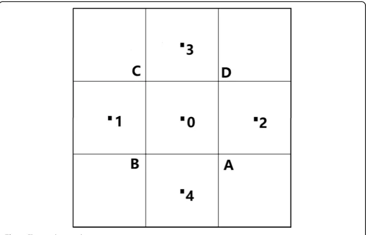
First, we consider an isotropic regular quadrilateral grid (quads.) stencils with aspect ratio AR= 1 as shown in Fig.4. The stencil only involves 5 points, i.e., point 0–point 4; the coordinates of those points are readily determined and will not be listed below.
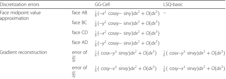
Exact face midpoint value and exact gradient at cell center 0 can be obtained by substituting the coordinates into the function f(x,y) and gradient ∇f respectively. The discretized face midpoint values are approximated as the average value of neighboring cell values for the GG-Cell method. The discretized gradients are reconstructed by the GG-Cell method and the LSQ method with basic stencils. Discretization errors are quantified by the difference between the discretized value and the exact value. Here, we directly present the discretization errors of both face midpoint value approximation and gradient reconstruction as follows.
In Table 2, both GG-Cell and LSQ-basic reconstructed gradients achieve
second-order accuracy and the absolute values of discretization error are identical. Special attention should be focused on the second-order accurate GG-Cell method; it is obvi-ous in this case that the second-order terms in the face midpoint value approximation will counterbalance each other in the discretized integral process which results in higher-than-first-order accurate GG gradient reconstruction. And the LSQ-basic method achieves second-order accuracy because it is equivalent to the central difference on Cartesian grids [29].
Following the analysis on regular quadrilateral grids, regular triangular grids (reg. tri.) and regular double-split triangular grids (reg. double-split tri.) can be considered in a
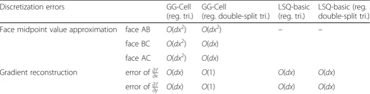
similar way. Grid stencils are sketched in Figs. 5 and 6. Brief results on discretization errors of gradient reconstruction and face midpoint value approximation are shown in Table3. Detailed results on discretization errors are provided inAppendix 2.
With reference to Table3and Table 8 inAppendix 2, it can be noted that on regular triangular grids, both GG-Cell and LSQ-basic reconstructed gradients achieve the first-order accuracy. However, on regular double split triangular grids, the GG-Cell method
degrades to 0th order (O(1)) because the accuracy of face midpoint value
approxima-tion on two faces (face BC and face AC) degrades to first-order and no counterbalance occurs under this circumstance. This conclusion is different from those reported in previous works, for example, in Ref. [7], Green-Gauss method and least-squares gradi-ent reconstruction were considered to produce similar results on regular meshes, and in Ref. [16], Green-Gauss methods were recognized insensitive to mesh regularity [16].
Further study on this problem shows that the accuracy degradation of GG-Cell method closely relates to mesh topology. If the face midpoint does not bisect the Table 2Discretization errors of gradient reconstruction and face midpoint value approximation (quads.)
Discretization errors GG-Cell LSQ-basic
Face midpoint value approximation
face AB 1 8ð−x
2cosxy−sinyÞdx2þ
Oðdx3Þ –
face BC 1
8ð−y2cosxy−sinxÞdx 2þ
Oðdx3Þ
face CD 1
8ð−x2cosxy−sinyÞdx 2þ
Oðdx3Þ
face AD 1
8ð−y2cosxy−sinxÞdx 2þ
Oðdx3Þ
Gradient reconstruction error of
∂f ∂x
1
6ðcosx−y3sinxyÞdx 2þ
Oðdx3Þ 1
6ðcosx−y3sinxyÞdx 2þ
Oðdx3Þ
error of
∂f ∂y
1
6ðcosy−x3sinxyÞdx 2þ
Oðdx3Þ 1
6ðcosy−x3sinxyÞdx 2þ
Oðdx3Þ
note:dxin the equations is the grid spacing (side length of the quadrilateral) in thex-direction
segment connecting the centers of two neighboring cells (as shown in Fig. 6), second-order accurate approximation of face midpoint value will be not achieved, and thus first-order gradient accuracy will not be maintained, as listed in Table3.
Accuracy degradation was also predicted by Mavriplis [10] when the segments
con-necting neighboring cell centers do not bisect the shared mesh edge. Sozer et.al [8] confirmed that the Green-Gauss approach with either simple or IDW face averaging is 0th order accurate by numerical gradient accuracy tests. In this paper, a similar phenomenon of accuracy degradation is observed, and furthermore, the fundamental reason is located on the accuracy of face midpoint value approximation. However, we will show next on curved meshes that the conclusion by Mavriplis is not complete enough and there exists at least one special case that does not comply with his statement but can still be explained by the theory proposed in this paper.
4.1.2 Meshes on the curved surface (curved mesh)
For typical isotropic grids on curved surfaces, the accuracy of face midpoint value approximation and gradient reconstruction methods are analyzed with the stencil sketched in Fig.7.
Fig. 6Regular double-split triangular grid stencils (AR= 1; reg. double-split tri.)
Table 3Discretization errors of gradient reconstruction and face midpoint value approximation
Discretization errors GG-Cell (reg. tri.)
GG-Cell
(reg. double-split tri.)
LSQ-basic (reg. tri.)
LSQ-basic (reg. double-split tri.)
Face midpoint value approximation face AB O(dx2)
O(dx2) – –
face BC O(dx2)
O(dx)
face AC O(dx2)
O(dx)
Gradient reconstruction error of∂f
∂x O(dx) O(1) O(dx) O(dx)
error of∂f
Firstly, following the definition of Diskin et al. [11], curvature induced mesh deform-ation is characterized by parameterΓ:
Γ¼jy1−y0j
y3−y0
j j¼R
−Rcoshθ 2hr ≈
Rh2θ 2hr ¼AR
hθ
2 ð21Þ
where yi is the y coordinate of point i in the Cartesian coordinate system, R is the
radius at cell center 0, hθandhrare mesh size in the circumferential direction and the
radial direction. AR=Rhθ/hr is the grid aspect ratio, for isotropic grids considered in
this paper,AR~O(1). We can see that whenΓ→0, point 0 and point 1 lie on the hori-zontal line, thus no curvature exists. On the contrary, when Γincreases, the curvature induced mesh deformation increases as well. Particularly, when we refine the grids at a specifiedAR,Γdecreases withhθdiminishing, and the curvature induced mesh
deform-ation can be ignored when the mesh is refined to a certain scale.
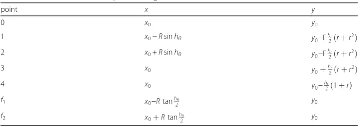
Coordinates of the stencil points are determined as follows in Table4:
in whichris the stretching ratio of the grids, for the isotropic grids considered in the paper,r= 1.
The gradient of function f(x,y) = sinx+ siny+ cosxy at cell 0 is reconstructed by
GG-Cell and LSQ-basic gradient reconstruction methods with AR= 1. The
discretization errors are shown in Table5.
From Table5, face midpoint value approximations of face AB and face CD are
first-order accurate which is not sufficient to produce first-first-order accurate gradient, however, Fig. 7Quadrilateral grids on a curved surface
Table 4Coordinates of stencil points in Fig.8
point x y
0 x0 y0
1 x0−Rsinhθ y0−Γhr
2ðrþr2Þ
2 x0+Rsinhθ y0−Γhr
2ðrþr2Þ
3 x0 y0þhr
2ðrþr2Þ
4 x0 y0−hr
2ð1þrÞ
f1 x0−Rtanhθ
2 y0
Table 5 Discretization errors of gradient reconstruction and face midpoint value approximation Discre tization errors GG-Cell (cur ved quads.) LSQ (curved qua ds.) Face mi dpoin t value app roxim ation face AB −
1R2
Γ ð cos y − x sin xy Þ hθ þ O ð h
2 Þθ
– face BC O ð h
2Þθ
face
CD
−
1R2
Γ ð cos y − x sin xy Þ hθ þ O ð h
2Þθ
face
DA
O
ð
h
2Þθ
Gra dient recon struction error of ∂
f ∂x
− R Γ ð xy cos xy þ sin xy Þ hθ þ O ð h
2Þθ
− R Γ ð xy cos xy þ sin xy Þ hθ þ O ð h
2Þθ
error
of
∂
f ∂y
−
Γð2
cos y − x sin xy Þ hθ þ O ð h
2 Þθ
− R Γ 2 ð 1 þ Γ 2Þ ðð y 2þ x 2Γ 2Þ cos xy þ sin x þ Γ 2sin y Þ hθ þ O ð h
we can still obtain the first-order gradient on isotropic quadrilateral grids on a curved surface. The reason is that the first-order terms counterbalance each other under this condition which can be seen from the discretization errors of face AB and face CD. Besides,Γbecomes a significant parameter in determining the true order of accuracy of gradient reconstruction methods. Second-order accurate gradient reconstruction can be obtained if Γ is so small that the first-order term O(Γhθ) is even smaller than the
second-order termOðh2θÞand thus it can be ignored during the evaluation of the order
of accuracy. This conclusion will be validated in the next sub-section via numerical tests on curved quadrilateral meshes.
4.2 Numerical tests of gradient reconstruction
In order to verify the accuracy analysis of the gradient reconstruction methods, numer-ical tests on typnumer-ical 2D isotropic grids are performed.
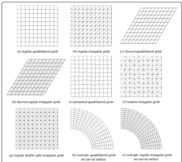
4.2.1 Grids and the approach of grid convergence study
Sketches of 9 typical grids are listed below in Fig.8.
(a) regular quadrilateral grids (quads.);
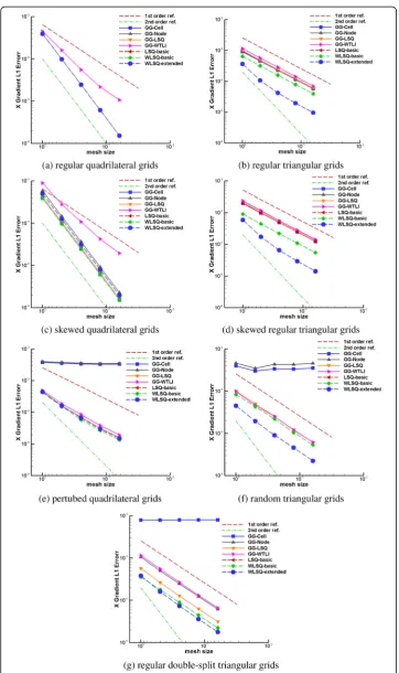
Fig. 9Convergence ofx-direction gradient of different grids and different reconstruction methods.aRegular quadrilateral grids.bRegular triangular grids.cskewed quadrilateral grids.dskewed regular triangular grids.e
(b) regular triangular grids (reg. tri.) derived from the regular quadrilateral grids by splitting the diagonal of each quadrangle in the same direction;
(c) skewed regular quadrilateral grids (skewed quads.); (d) skewed regular triangular grids (skewed reg. tri.);
(e) perturbed quadrilateral grids (perturbed quads.) with grid nodes shifting from their initial location by a random but limited fraction of local mesh size. Specifically, grid node perturbation in this paper is defined asrh/4, wherer∈[−1, 1] is a random number andhis the local mesh size [11–13];
(f) random triangular grids (rand. tri.) derived from randomly splitting the diagonal of the regular quadrilateral grids (left diagonal and right diagonal appear with equal probability);
(g) regular double-split triangular grids (reg. double-split tri.) derived from regular quadrilateral grids by double splitting the diagonal of each quadrangle in the same direction, i.e., splitting in the left and right diagonal respectively;
(h) isotropic quadrilateral grids on a curved surface (curved quads.); (i) isotropic regular triangular grids on a curved surface (curved tri.);
Grid convergence studies are carried out on a series of consistently refined grids. In-stead of shrinking the domain [19], mesh size is halved in a fixed domain by doubling the number of grid points on the boundary edges. The order of accuracy of gradient re-construction is obtained asymptotically with the decrease of the mesh size. Here the mesh size is defined as [15]
h¼ Vtotal ndof
1
d
ð22Þ
whereVtotalis the total volume of all cells in the domain,ndofis the number of degrees
of freedom in the mesh, for cell-centered schemes, ndof is set to the number of cells,
andddenotes the spatial dimension.
The flow function for gradient numerical tests is chosen to be a scalar manufactured solution [15] with 8 constant coefficientsϕ0,ϕx,ϕy,ϕxy,αϕx,αϕy,αϕxy,L:
Fig. 10Convergence of x-direction gradient of different grids and different reconstruction methods.h
ϕðx;yÞ ¼ϕ0þϕx sin αϕxπx
L
þϕy sin αϕyπy
L
þϕxy cos
αϕxyπxy L2
ð23Þ
Discretization errors are quantified by the difference between the exact gradient and the discretized one. The L1 norms, as shown in Eq. (24), of discretization error are calculated and plotted as a function of mesh size to study the convergence of discretization error. Here, theL2andL∞norms, as shown in Eqs. (25) and (26), can also
be adopted since they have the same performance on self-similar grids and will not lead to essentially different results on currently considered grids which are generally self-similar. So onlyL1norms are listed in the following context.
L1¼ XN
i¼1
fi−fi;exact
N ð24Þ
L2¼ XN
i¼1
fi−fi;exact
2
N
0 B B B B @
1 C C C C A
1=2
ð25Þ
L∞¼ maxfi−fi;exact ð26Þ
The order of accuracy (OOA) p can be determined by comparing discretization
er-rors between two consistently refined grids (E1andE2) as:
p¼ ln E2
E1
ln h2 h1
ð27Þ
4.2.2 Numerical results
Figure 9 illustrates the grid convergence performance of x-direction gradient
discretization error (L1 norm) for different meshes with different gradient reconstruc-tion methods. Overall agreement is observed between mathematical analyses and numerical tests.
Numerical results in Fig.9a-d show that all gradient reconstruction methods produce at least first-order gradient on regular quadrilateral grids and regular triangular grids and their skewed counterparts. Mesh skewness does not cause degradation of the order of accuracy since skewness alone does not lead to violation of the face midpoint value condition. However, it doesn’t necessarily imply that mesh skewness does not influence gradient or solution accuracy. Skewness, in fact, was demonstrated a key factor deteri-orating the solution accuracy of inviscid flow simulation by the authors [30].
Figure 9e-g show that the GG-Cell gradient reconstruction method degrades to 0th
Besides, GG-Node gradient reconstruction method also suffers from accuracy degrad-ation on random triangular grids and perturbed quadrilateral grids as shown in Fig. 9e and f. However, other GG methods that ensure second-order accurate face midpoint value approximation, such as GG-LSQ, GG-WTLI, maintain at least first-order gradient accuracy on all tested isotropic grids.
Meanwhile, as shown in Fig. 10h, gradient accuracy of GG-Cell method reaches
second order on isotropic quadrilateral grids on a curved surface which is consist-ent with previous analysis on the curved mesh. And all methods produce at least first-order gradient on curved quadrilateral grids and curved triangular grids. This confirms that other parameters such as curvature induced mesh deformation also play an important role in determining the actual order of accuracy of gradient re-construction. And the condition whether the face midpoint bisects the segment connecting the neighboring cells, as bisection fails on the curved mesh, is not ne-cessary for GG-Cell methods to be at least first-order accurate.
Fig. 11Density contour of Euler manufactured solutions on different geometries.aEuler manufactured solution on flat geometry.bEuler manufactured solution on curved geometry.cEuler manufactured solution on skewed geometry
These results verify the previous conclusion that the fundamental reason of accuracy degradation of GG methods is not achieving second-order accurate face midpoint value approximation.
Numerical tests of gradient reconstruction methods based on least-squares approach indicate that these methods are at least first-order accurate on all tested isotropic grids regardless of mesh type, mesh perturbation, surface curvature, and skewness.
In terms of absolute magnitude of gradient discretization error and comparison of these gradient reconstruction methods, WLSQ method with extended stencil ex-hibits the lowest level of error on all tested grids except isotropic quadrilateral grids on curved surface, while other methods exhibit erratic behaviors and it is hard to identify the best method for all grids which, in fact, is not the goal of the current study.
5 Method of manufactured solutions
In order to quantify solution errors, we need an exact solution for the governing equations. Common exact solutions for real physical flows are either too difficult to ob-tain, or if exist, they are often solutions of the simplified equations and do not exercise all terms in the complete equations.
Therefore, except for simple exact solutions, a more powerful tool, the Method of Manufactured Solutions (MMS) [18,31], is adopted in this paper. In a general proced-ure of MMS, non-trivial but analytic solutions are manufactproced-ured without being concerned about its physical realism since accuracy analysis is a purely mathematical exercise, and the analytic solutions should be complex enough to exercise all terms in the governing equations being tested.
Instead of solving the original partial differential equation (PDE), we solve the
equations added with an analytic source term. Considering an analytic solution Qm,
and substituting the solution into the governing PDE, then we can obtain an analytic source term Sm. It is obvious that the analytic solution Qmis the exact solution of the modified equation, i.e., the original equation added with an analytic source term, as Table 6Validation of the MMS procedure
Grid (a) grid cells Inviscid vortex Euler MMS Grid (b) grid cells Inviscid vortex Euler MMS
L1Error OOA L1Error OOA L1Error OOA L1Error OOA 20 × 20 1.45e-02 – 1.22e-03 – 800 1.38e-02 – 6.14e-04 –
40 × 40 3.11e-03 2.22 2.15e-04 2.50 3200 3.14e-03 2.14 1.60e-04 1.94
80 × 80 6.80e-04 2.19 4.78e-05 2.17 12,800 7.02e-04 2.16 4.00e-05 2.00
160 × 160 1.57e-04 2.11 1.16e-05 2.04 51,200 1.66e-04 2.08 9.94e-06 2.01
320 × 320 3.85e-05 2.03 2.86e-06 2.02 204,800 4.05e-05 2.04 2.47e-06 2.01
Grid (e) grid cells Inviscid vortex Euler MMS Grid (f) grid cells Inviscid vortex Euler MMS
L1Error OOA L1Error OOA L1Error OOA L1Error OOA 20 × 20 1.41e-02 – 1.89e-03 – 800 1.60e-02 – 2.62e-03 –
40 × 40 5.61e-03 1.33 8.79e-04 1.10 3200 5.04e-03 1.67 1.03e-03 1.35
80 × 80 1.74e-03 1.69 4.05e-04 1.12 12,800 1.76e-03 1.52 5.60e-04 0.88
160 × 160 7.53e-04 1.21 2.18e-04 0.89 51,200 7.06e-04 1.32 2.48e-04 1.18
shown in Eq. (28). Solving the modified equation, we can get the discretized numerical solution. Thus the solution errors can be quantified by comparing the exact manufac-tured solution and the numerical solution.
∂Q
∂t þ∇Fc−∇Fv¼Sm ð28Þ
In dealing with the analytic source term, two major approaches were presented in
previous work. Katz [15] reported second-order accurate source term discretization,
while Roache [18] suggested symbolic manipulation of the source term. In this paper, we adopt the symbolic manipulation to obtain the exact expression of the source term. Dirichlet boundary conditions are implemented.
5.1 Euler manufactured solution
Quantification of discretization error is accomplished by a vector Euler manufactured
solution [15] for two-dimensional (2D) cases, and the manufactured solutionQm has
the following components:
Fig. 13Convergence of density discretization error on different grids with different reconstruction methods.a
Regular quadrilateral grids.bRegular triangular grids.cSkewed quadrilateral grids.dSkewed regular triangular grids.ePerturbed quadrilateral grids.fRandom triangular grids.gRegular double-split triangular grids.h
ρðx;yÞ ¼ρ0þρx sin αρxπx
L
þρy sin αρyπy L
þρxy cos αρxyπxy L2
u xð ;yÞ ¼u0þux sin αuxπx
L
þuy sin αuyπy L
þuxy cos αuxyπxy L2
v xð ;yÞ ¼v0þvxsin αvxπx
L
þvy sin αvyπy L
þvxy cos αvxyπxy L2
P xð ;yÞ ¼P0þPx sin αPxπx
L
þPy sin αPyπy L
þPxy cos αPxyπxy L2
ð29Þ
in which ρ0,ρx,ρy,ρxy,αρx,αρy,αρxy,Land corresponding parameters in other
compo-nent equations are constant coefficients. Analytic source terms are derived by Mathe-matica symbol manipulation. Modified Euler equation (added with an analytic source term) is solved to determine the discretized solutions. Initial density contours are plotted in Fig.11.
5.2 Validation of MMS procedures
Validation of MMS procedures is performed by comparing the order of accuracy (OOA) obtained by the MMS procedure and an exact solution case. The exact solution adopted in this paper is a 2D inviscid isentropic vortex. Exact initial conditions are specified according to Ref. [8,32] as
u¼− ε
2πðy−y0Þe
0:5 1ð−r2Þ v¼ ε
2πðx−x0Þe
0:5 1ð−r2Þ T ¼1−ðγ−1Þε
2
8γπ2 e 1−r2
ð Þ
ρ¼Tγ1−1;p¼ργ;S¼p=ργ ¼1
ð30Þ
where r¼
ffiffiffiffiffiffiffiffiffiffiffiffiffiffiffiffiffiffiffiffiffiffiffiffiffiffiffiffiffiffiffiffiffiffiffiffi ðx−x0Þ2þ ðy−y0Þ
2 q
, the vortex strength is taken asε= 5.0, and the vortex
core is located at (x0,y0) = (0, 0). Eq. (30) is an exact solution for Euler equations thus can be adopted to verify and validate the MMS procedures. Initial density contour of a 2D inviscid vortex is plotted in Fig.12.
Grid convergence studies on 4 types of grids, i.e., grids (a), (b), (e) and (f) in Fig. 8, are performed with same discretization scheme, and the OOA of the numerical
solu-tion is determined. Table 6 shows theL1error and the OOA obtained by the inviscid
vortex and by the MMS procedure with a Euler manufactured solution. It demonstrates that the Euler MMS procedure obtains the same OOA as the exact solution case.
6 Effects on the accuracy of inviscid flow simulation
Previous sections examined the accuracy of various gradient reconstruction methods, identified accuracy degradation for certain methods and verified former mathematical conclusions. However, poor gradient reconstruction accuracy does not necessarily imply large discretization error for the governing equations [10, 13]. The gradient ac-curacy and the FV discretization acac-curacy was thought to be unrelated. In this section, the effects of gradient accuracy on simulation of inviscid flows are considered. Solution errors are quantified by the validated Euler MMS procedure.
error of the Euler MMS tests with different gradient reconstruction methods, in which
‘1st order’implies the numerical schemes adopting a constant reconstruction (i.e., Eq. (3)), and‘1storder ref.’and‘2ndorder ref.’are 1st order and 2nd order reference lines.
Figure13a-d show that FV schemes on grids (a)-(d) are second-order for all gradient reconstruction methods and the solution accuracy (absolute value of density discretization error) are nearly the same even though the gradient reconstructions have different accuracy as shown in Fig.9a-d.
Figure 13e-g indicate that the schemes employing GG-Cell gradient reconstruction
method degrade to first-order on grids (e)-(g) (perturbed quadrilateral grids, random tri-angular grids, and regular double-split tritri-angular grids). The schemes employing GG-Node method also suffer from accuracy deterioration on these grids except regular double-split triangular grids. It proves that first-order accurate gradient reconstruction is necessary to maintain second-order FV schemes. These results clearly show that 0th order GG methods will lead to first-order FV schemes and generate a much higher level of absolute error.
In Fig.13e-g, we also notice that even though gradient reconstruction of GG methods degrades to 0th order and the corresponding FV schemes degrade to 1st order, these schemes still yield a lower level of absolute error than the pure first-order FV scheme with a constant reconstruction. In other words, 0th order gradient reconstruction is still better than constant reconstruction.
Figure 13h-i show that all FV schemes on curved quadrilateral grids and curved tri-angular grids are second-order which confirms again the conclusion that first-order gradient reconstruction is necessary to yield second-order FV discretization.
Besides, FV discretization employing LSQ methods (LSQ-basic, WLSQ-basic, and WLSQ-extended) is always second-order accurate since LSQ gradient reconstruction is always at least first-order on arbitrary unstructured grids. Meanwhile, we also notice again that when gradient reconstruction achieves the first-order accuracy as shown in
Fig. 9, the absolute error of gradient reconstruction does not directly imply the
absolute error of numerical solution accuracy.
Although not considered in this paper, the computational efficiency of these schemes differs very much from each other. Preliminary studies on the complexity and efficiency
of FV schemes were reported in previous studies [12, 13], and we will further study these issues in future work.
7 Conclusions and future work
Gradient reconstruction based on the Green-Gauss theorem (the GG methods) and the least-squares approaches (the LSQ methods) are analyzed both mathematically and nu-merically. Mathematical derivations reveal that, for gradient reconstruction based on the Green-Gauss theorem (the GG methods), if the summation of first-and-lower-order terms does not counterbalance in the discretized integral process, which rarely occurs, second-order accurate approximation of face midpoint value is necessary to produce at least first-order accurate gradient. However, gradient reconstruction methods based on the least-squares approach (LSQ methods) are at least first-order on arbitrary unstruc-tured grids. These conclusions are verified by discretization error analysis on typical grid stencils and numerical accuracy tests on various types of isotropic grids.
Fig. 15Stencils for GG-Node method
If the face midpoint value condition is not satisfied, GG methods, such as GG-Cell and GG-Node method on irregular or perturbed mesh, will degrade to 0th order. Nu-merical tests indicated that on all tested isotropic grids, LSQ methods maintain at least first-order accurate gradient reconstruction.
In terms of gradient accuracy effects on the accuracy of inviscid flow simulation, it demonstrates that first-order accurate gradient is necessary to yield second-order FV discretization. The GG methods that produce the 0th order gradient should not be pre-ferred in terms of simulation accuracy for practical flow simulations since they yield first-order FV discretization and generate much higher solution error. While second-order FV discretizations are ensured for all LSQ methods on all types of grids.
For gradient methods that yield the first-order gradient, which is sufficient for second-order FV schemes, it demonstrates that the gradient accuracy does not directly imply the numerical solution accuracy.
Previous work reported that GG methods may be more robust than LSQ methods on anisotropic grids on the curved surface [10,11, 26, 27]. Future work will focus on the performance of gradient reconstruction methods on anisotropic and stretched grids with high aspect ratio and surface curvature for viscous flow simulations. Attempts on possible modifications of GG methods according to the face midpoint value condition will be carried out to improve the gradient and solution accuracy. While for the LSQ methods, improving robustness on high aspect ratio grids with surface curvature is worthful work.
8 Appendix 1
According to the approach for face midpoint value approximation, the GG methods can be categorized (but not limited) into the following types:
(a) cell-based GG methods (GG-Cell), using a simple average value of face neighboring cells as face midpoint value;
(b) nodal-based GG methods (GG-Node), using a simple average value of node surrounding cells as face nodal value;
(c) inverse distance weighted GG methods (GG-IDW); (not considered in this paper)
Table 7 Discretization errors of gradient reconstruction and face midpoint value approximation (reg. tri) Discre tization errors GG-Ce ll LSQ-basic Face mi dpoin t value app roxim ation face AB
1ð72
− ð − 2 x þ y Þ 2 cos xy − sin x − 4 sin y þ 4 sin xy Þ dx 2 þ O ð dx 3 Þ – face BC
1ð72
− ð x − 2 y Þ 2 cos xy − 4 sin x − sin y þ 4 sin xy Þ dx 2þ O ð dx 3Þ face AC
1ð72
− ð x þ y Þ 2 cos xy − sin x − sin y − 2 sin xy Þ dx 2þ O ð dx 3Þ Gra dient recon struction error of ∂
f ∂x
1ðð6
2 x − y Þ y cos xy − sin x þ 2 sin xy Þ dx þ O ð dx 2Þ 1ðð6
2 x − y Þ y cos xy − sin x þ 2 sin xy Þ dx þ O ð dx 2Þ error of ∂
f ∂y
1ð−6
x ð x − 2 y Þ cos xy − siny þ 2 sin xy Þ dx þ O ð dx 2Þ 1ð−6
Table 8 Discretization errors of gradient reconstruction and face midpoint value approximation (reg. Double-split tri) Discre tization errors GG-Ce ll LSQ-basic Face mi dpoin t value app roxim ation face AB
1ð72
− x 2cos xy − sin y Þ dx 2þ O ð dx 3Þ – face BC
1ð12
cos x − cos y þð x − y Þ sin xy Þ dx þ O ð dx 2 Þ face AC
1ð12
− cos x − cos y þð x þ y Þ sin xy Þ dx þ O ð dx 2Þ Gra dient recon struction error of ∂
f ∂x
1ð3
cos x − y sin xy Þþ O ð dx Þ
1ð−3
xy cos xy − sin xy Þ dx þ O ð dx 2Þ error of ∂
f ∂y
1ð−3
cos y þ x sin xy Þþ O ð dx Þ
1ð18
(d) GG methods based on least-squares face interpolation (GG-LSQ), using LSQ interpolation to calculate face midpoint value;
(e) GG methods based on weighted tri-linear face interpolation (GG-WTLI), using weighted tri-linear interpolation to calculate face midpoint value.
Descriptions of these methods for cell-centered data structure are reviewed in the following text.
(1) GG-Cell
As shown in Fig. 14, GG-Cell method approximates face midpoint value by simply
averaging cell values of direct neighbors.
Uij¼UiþUj
2 ð31Þ
Simple algebraic average in Eq. (31) can be replaced by distance or volume-weighted interpolation as
Uij¼wiUiþwjUj ð32Þ
where wi and wj are distance or volume weights. Neither weighted interpolation nor
simple algebraic averaged interpolation guarantees second-order face midpoint approxi-mation. GG-Cell method with a simple algebraic average is considered only in this paper.
(2) GG-Node
As shown in Fig.15, GG-Node methods approximate face midpoint value by a simply
algebraic average of nodal values, as shown in Eq. (33). Nodal values are obtained by weighted interpolation of surrounding cells, either equal-weighted, as Eq. (34) shows, or distance/volume-weighted.
Uij¼UAþUB
2 ð33Þ
UA¼ 1
NðU1þU2þ⋯þUNÞ ¼ 1 N
XN
j¼1
Uj ð34Þ
where UA and UB are nodal values of the computed face, in this 2D case, a face/edge
consists of two nodes. Similar to GG-Cell methods, neither weighted interpolation nor simple averaging interpolation guarantees second-order face midpoint value approxima-tion. The GG-Node method with equal-weighted interpolation is considered in this paper.
(3) GG-IDW[8]
As shown in Fig.16, GG-IDW method approximates face midpoint value by inverse
distance weighted interpolation.
ϕf ¼
XN
i¼1 ϕi= ri
*
2
XN
j¼1
1=r*j
2 ð35Þ
cell point i. This method is similar to GG-Node with distance weighted nodal value interpolation where nodal values are obtained by inverse distance weighted interpolation. So this method is only introduced and no further consideration will be taken in this paper.
(4) GG-LSQ[8]
Also as shown in Fig. 16, GG-LSQ method approximates face midpoint value by
weighted least square approach. Value at stencil pointican be obtained by value at face midpointfwith a gradient interpolation, as shown in Eq. (36).
ϕi¼ϕf þ
∂ϕ
∂xfΔxiþ
∂ϕ
∂yfΔyiþ
∂ϕ
∂zfΔziþh:o:t: ð36Þ
whereΔxi, Δyi, Δziare the components of the distance vector. With Eq. (36),
interpolat-ing all stencil points from face midpoint and neglectinterpolat-ing the high order terms, we obtain an over-determined system, as shown in Eq. (37). Solving the over-determined system, we can get the face midpoint value with a minimum-error interpolation of each stencil point.
θ1 θ1Δx1 θ1Δy1 θ1Δz1 θ2 θ2Δx2 θ2Δy2 θ2Δz2
⋮ ⋮ ⋮ ⋮
θj θjΔxj θjΔyj θjΔzj
⋮ ⋮ ⋮ ⋮
θN θNΔxN θNΔyN θNΔzN
2 6 6 6 6 6 6 4 3 7 7 7 7 7 7 5 ϕf ∂ϕ
∂xf
∂ϕ
∂yf
∂ϕ
∂zf
2 6 6 6 6 6 6 6 4 3 7 7 7 7 7 7 7 5 ¼ θ1ϕ1 θ2ϕ2 ⋮ θjϕj
⋮ θNϕN
2 6 6 6 6 6 6 4 3 7 7 7 7 7 7 5 ð37Þ
(5) GG-WTLI[8]
As shown in Fig. 17, GG-WTLI method approximates face midpoint value by
weighted tri-linear interpolation. Specifically, face midpoint value at f is interpolated from three surrounding non-collinear stencil points with linear regression.
x1 x2 x3
y1 y2 y3
1 1 1
2 4
3 5 CC12
C3 2 4
3 5¼ xfyf
1
2 4
3
5 ð38Þ
ϕf ¼C1ϕ1þC2ϕ2þC3ϕ3 ð39Þ
Monotone interpolation can be obtained if face midpointflocates within the triangle composed by the three non-collinear stencil points. Some other possible triangles for tri-linear interpolation are shown Fig. 17b. The final approximation of face midpoint value can be obtained by weighting each triangle’s stencil coefficients with the inverse distance from the triangle center to the face midpoint.
9 Appendix 2
The detailed expressions of discretization errors of gradient reconstruction and face midpoint value approximation are given below.
Table 8 shows the discretization properties of regular double-split triangular grids (reg. double-split tri. as shown in Fig.8g). It indicates that for the GG-Cell method, face midpoint value approximations on two faces (face BC and face AC) degrade to first-order which is not sufficient to yield first-first-order gradient reconstruction as the errors of gradient reconstruction in the table are 0th order. However, the LSQ method with basic stencils still achieves first-order gradient reconstruction.
Acknowledgments
This work is supported by National Natural Science Foundation of China [grant numbers 11532016, 91530325].
Authors’contributions
The contribution of the authors to the work is equivalent. All authors read and approved the final manuscript.
Funding
National Natural Science Foundation of China [grant numbers 11532016, 91530325].
Availability of data and materials
All data generated or analyzed during this study are included in this published article.
Competing interests
The authors declare that they have no competing interests.
Received: 31 May 2019 Accepted: 21 August 2019
References
1. Jameson A, Schmidt W, Turkel E (1981) Numerical solutions of the Euler equations by finite volume methods using Runge-Kutta time-marching schemes. 14th Fluid and Plasma Dynamics Conference, Palo Alto, pp 81–1259 2. Ni RH (1982) A multiple-grid scheme for solving the Euler equation. AIAA J 20(11):1565–1571
3. Roe PL (1987) Error estimates for cell-vertex solution of compressible Euler equations. NASA Contract Rep:178235 4. Giles MB (1989) Accuracy of node-based solutions on irregular meshes. In: 11th international conference on numerical
methods in fluid dynamics, vol 323, pp 369–373
5. Lindquist DR (1988) A comparison of numerical schemes on triangular and quadrilateral meshes. Maters’Thesis, Massachusetts Institute of Technology. Cambridge, Massachusetts.
6. Barth TJ, Jespersen DC (1989) The design and application of upwind schemes on unstructured meshes. 27th Aerospace Sciences Meeting, Reno, pp 89–0366
7. Aftosmis M, Gaitonde D, Tavares TS (1995) Behavior of linear reconstruction techniques on unstructured meshes. AIAA J 33(11):2038–2049
8. Sozer E, Brehm C, Kiris CC (2014) Gradient calculation methods on arbitrary polyhedral unstructured meshes for cell-centered CFD solvers. 52nd Aerospace Sciences Meeting, National Harbor, pp 2014–1440
9. Smith TM, Barone MF, Bond RB et al (2007) Comparison of reconstruction techniques for unstructured mesh vertex centered finite volume schemes. 18th AIAA Computational Fluid Dynamics Conference, Miami, pp 2007–3958 10. Mavriplis DJ (2003) Revisiting the least-squares procedure for gradient reconstruction on unstructured meshes. 16th
AIAA Computational Fluid Dynamics Conference, Orlando, pp 2003–3986
11. Diskin B, Thomas JL (2008) Accuracy of gradient reconstruction on grids with high aspect ratio. NIA Rep 12. pp. 1–25 12. Diskin B, Thomas JL, Nielsen EJ et al (2009) Comparison of node-centered and cell-centered unstructured finite-volume
discretizations: viscous fluxes. 47th AIAA Aerospace Sciences Meeting including The New Horizons Forum and Aerospace Exposition, Orlando, pp 2009–0597
13. Diskin B, Thomas JL (2010) Comparison of node-centered and cell-centered unstructured finite-volume discretizations: inviscid fluxes. 48th AIAA Aerospace Sciences Meeting Including the New Horizons Forum and Aerospace Exposition, Orlando, pp 2010–1079
14. Katz A, Sankaran V (2012) High aspect ratio grid effects on the accuracy of Navier-stokes solutions on unstructured meshes. Comput Fluids 65:66–79
15. Katz A, Sankaran V (2011) Mesh quality effects on the accuracy of CFD solutions on unstructured meshes. J Comput Phys 230:7670–7686
16. Diskin B, Thomas JL (2012) Effects of mesh regularity on accuracy of finite-volume schemes. 50th AIAA Aerospace Sciences Meeting including the New Horizons Forum and Aerospace Exposition, Nashville, pp 2012–0609
17. Betchen LJ, Stratman AG (2010) An accurate gradient and hessian reconstruction method for cell-centered finite volume discretizations on general unstructured grids. Int J Numer Methods Fluids 62:945–962
18. Roache PJ (2002) Code verification by method of manufactured solutions. Trans ASME 124:4–10
19. Herbert S, Honey EAL (2005) I shrunk the grids! A new approach to CFD verification studies. 43rd AIAA Aerospace Sciences Meeting and Exhibit, Reno, pp 2005–2685
20. Diskin B, Thomas JL (2007) Accuracy analysis for mixed-element finite-volume discretization schemes. NIA Tech Rep 8:2007 21. Thomas JL, Diskin B, Rumsey CL (2008) Towards verification of unstructured-grid solvers. 46th AIAA Aerospace Sciences
Meeting and Exhibit, Reno, pp 2008–2666
23. He X, Zhang LP, Zhao Z et al (2013) Research and development of structured/unstructured hybrid CFD software. Trans Nanjing Univ Aeronaut Astronaut 30:116–120
24. He X, He XY, He L et al (2015) HyperFLOW: a structured/unstructured hybrid integrated computational environment for multi-purpose fluid simulation. Procedia Eng 126:645–649
25. Blazek J (2001) Computational fluid dynamics: principles and application. Elsevier, Butterworth-Heinemann 26. Roe PL (1981) Approximate Riemann solvers, parameter vectors, and difference schemes. J Comput Phys 43:357–372 27. Shima E, Kitamura K, Haga T (2013) Green–gauss weighted-least-squares hybrid gradient reconstruction for arbitrary
Polyhedra unstructured grids. AIAA J 51(11):2740–2747
28. Nishikawa H (2019) Efficient gradient stencils for robust implicit finite-volume solver convergence on distorted grids. J Comput Phys 386:486–501
29. Moukalled F, Mangani L, Darwish M (2016) The finite volume method in computational fluid dynamics: an advanced introduction with OpenFOAM and Matlab. Springer International Publishing, Switzerland
30. Wang NH, Zhang LP, Ma R, et al (2016) Mesh quality effects on the accuracy of gradient reconstruction and inviscid flow simulation on isotropic unstructured grids. Chinese J Comput Mech, 34(5):555–563
31. Roache PJ, Steinberg S (1984) Symbolic manipulation and computational fluid dynamics. AIAA J 22(10):1390–1394 32. Pulliam T (2011) High order accurate finite-difference methods: as seen in OVERFLOW. 20th AIAA Computational Fluid
Dynamics Conference, Honolulu, pp 2011–3851
Publisher’s Note
![Fig. 2 LSQ basic stencils [8] (cell 0–6)](https://thumb-us.123doks.com/thumbv2/123dok_us/9581147.1940919/8.595.120.478.478.720/fig-lsq-basic-stencils-cell.webp)
![Fig. 3 LSQ extended stencils [8] (cell 0–10)](https://thumb-us.123doks.com/thumbv2/123dok_us/9581147.1940919/9.595.118.479.88.341/fig-lsq-extended-stencils-cell.webp)