R E S E A R C H A R T I C L E
Open Access
On the effect of the contact surface
definition in the Cartesian grid finite
element method
José Manuel Navarro-Jiménez
∗, Manuel Tur, Francisco Javier Fuenmayor and
Juan José Ródenas
*Correspondence: [email protected]
Centro de Investigación en Ingeniería Mecánica, Departamento de Ingeniería Mecánica y de Materiales, Universidad Politécnica de Valencia, Camino de Vera s/n, 46022 Valencia, Spain
Abstract
The definition of the surface plays an important role in the solution of contact problems, as the evaluation of the contact force is based on the measure of the gap between the solids. In this work three different methods to define the surface are proposed for the solution of contact problems within the framework of the 3D Cartesian grid finite element method. A stabilized formulation is used to solve the contact problem and details of the kinematic description for each surface definition are provided. The three methods are compared solving some numerical tests involving frictionless contact with finite and small deformations.
Keywords: Contact, Immersed boundary, cgFEM, NURBS
Introduction
In recent years some alternatives to standard Finite Element methods have been developed under the category of immersed boundary methods [1–3], also known as fictitious or embedded domain methods. The common idea in these methods is that the FE mesh is obtained by discretizing a simple domain (usually cuboid) which fully embeds the analysis domain, but is independent of the analysis boundaries, which may be complex. Within this category is the Cartesian grid finite element method (cgFEM) for solving elasticity problems in 2D [4] and 3D [5]. The main differentiating features of cgFEM with respect to other immersed boundary methods are that the cgFEM is able to consider the CAD geometry (represented by NURBS) for the numerical integration and the use of a stabilized Lagrange multiplier method for the imposition of Dirichlet boundary conditions (see [5] and [6] for further details).
In order to solve the contact problem with cgFEM we use a stabilized Lagrangian formu-lation first presented in [7]. The method has similarities with Nitsche-based formulations proposed in [8–11] with a relevant difference in the stabilizing stress field. In our case we use a smooth field calculated with the Zienkiewicz and Zhu Superconvergent patch recovery (SPR) technique [12–14]. In a first approach, the developed contact formulation was applied to cgFEM considering a linear facet discretization of the boundary, based on the intersections between the Cartesian grid with the CAD geometry.
©The Author(s) 2018. This article is distributed under the terms of the Creative Commons Attribution 4.0 International License (http://creativecommons.org/licenses/by/4.0/), which permits unrestricted use, distribution, and reproduction in any medium, provided you give appropriate credit to the original author(s) and the source, provide a link to the Creative Commons license, and indicate if changes were made.
Several attempts to enhance the definition of the contact boundaries have been devel-oped in the framework of body-fitted meshes, usually known as surface smoothing, using diverse techniques such as Hermite, Bezier spline and NURBS interpolations [15–18], Gregory patches [19] or Nagata patches [20]. It is proven in these works that the enhance-ment of the contact surfaces results in more accurate solutions and increased robustness of the contact algorithm. A relevant contribution in the consideration of CAD geometries is the isogeometric analysis [21] (and its applications in contact simulation, e.g. [22,23]), in which the basis functions for the approximation of the solution are the same used for the CAD definition. There are also NURBS-enriched formulations as in [24,25], where isogeometric basis functions are included only in the contact elements.
As the cgFEM is able to consider the CAD geometry, it seems appropriate to use this surface definition to improve the gap measure. In [26] the deformed surface is defined as a combination of the undeformed CAD geometry and the finite element displacement field. This paper can be considered as an extension of [26], where we study the effect of the surface definition (hence the contact gap) when solving frictionless contact problems with cgFEM. In addition to the previous approaches, linear facets and a combination of FE solution and NURBS surface, in this work we propose a new method in which the deformed configuration is defined as a NURBS surface, i.e., the control points of the original CAD surface are updated such that the new configuration fits the finite element displacement field of the contact surface.
The paper is structured as follows: in “Contact kinematics” section the kinematic vari-ables of the problem are stated. The different alternatives to define the contact surface are presented in “Discretization of contact kinematics” section. The formulation used to solve the contact problem is described in “Stabilized Lagrangian contact formulation” sec-tion. Finally the different methods are compared with some numerical tests in “Numerical examples” section.
Contact kinematics
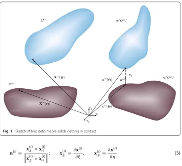
Figure1shows the undeformed and deformed configurations of two solids(i)coming in
contact. The indexes(1),(2)represent the so-calledslaveandmasterbodies respectively. (i)
c is the part of body (i) that can interact with the other body. Let X be the initial
configuration of a given material point in(i), i= 1,2. We describe the motion of(i) with the mappingϕ :−→R3. Thereforex(i)= ϕ
X(i), tfor a given point at timet.
Since we are solving quasi-static problems, we will omit the time variable and assume that the load increments are small enough. Then, the position vector for any point in(i)is given as
x(i)=ϕX(i) (1)
To enforce the contact constrain, a pair of points x(1), x(2) is defined such that the following equation is fulfilled:
x(2)(2)=g
Nn(1)+x(1)
(1); x(1)∈(1)
c , x(2)∈(2)c (2)
where(i)≡(ξ,η)(i)are the convective coordinates of(ci)andgN is the contact normal
gap. The normal vector to the surface is obtained from the tangent vectors to the surface
Fig. 1 Sketch of two deformable solids getting in contact
n(i)= x (i) ,ξ ×x,(ηi)
x(i)
,ξ ×x,η(i)
; x,ξ(i)= ∂x
(i)
∂ξ , x,η(i)= ∂x(i)
∂η (3)
We use a ray-tracing scheme to build the contact pair, so, x(1) remains fixed and Eq. (2) has the unknowns(2) andgN. The method for solving this equation depends on
the parametric transformationx(2)((2)). Equation (2) can be directly solved for linear facets. However, if the surface is defined using rational transformations (e.g. NURBS) (2) becomes non-linear, so we use a Newton-Raphson scheme.
From now onwards we assume that (ξ,η)(2)≡(ξ,η). We can now take variations in (2): δx(2)(ξ,η)=δg
Nn(1)+gNδn(1)+δx(1) (4)
Taking into account thatδn(1)·n(1)=0,n(1)·n(1)=1 and projecting Eq. (4) inton(1) we obtain the variation of the normal gap:
δgN =
δx(2)(ξ,η)−δx(1)·n(1) (5)
Discretization of contact kinematics
The finite element (FE) approximation of these continuum variables introduces two important sources of error. One is related to the discretization of the analysis domain hwhich usually differs from the original. The approximation of the continuum
dis-placement with the FE variableuh introduces the discretization error. We define this field from the nodal valueu using linear shape functions,uh = Nkuk, whereuk is the
displacement of nodek.
a b c
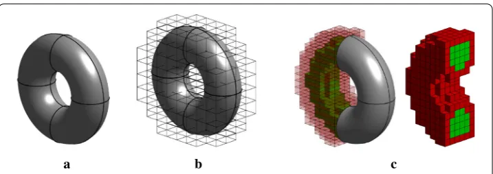
Fig. 2 Disctretization mesh of a torus in cgFEM. In green, elements internal to the domain. In red, elements cut by the boundary (boundary elements). Elements completely outside the domain are not considered during the analysis.aPhys. domain.bDiscretizationh.cInternal and boundary elements
c b
a
Fig. 3 Surface and volume discretization using the Marching Cubes algorithm and cgFEM.aInside-outside test of nodes using intersections data.bMarching Cubes topology.cVolume (green) and surface (red) quadratures considering CAD geometry
The second alternative, first introduced in [7], includes the CAD definition of(ci) in
the reference configuration, combined with the FE approximation of the displacements. Finally we present an alternative in which the CAD surface is deformed such that it fits the FE solution.
Previous considerations regarding cgFEM
Surface topology with the Marching cubes algorithm
In body-fitted contact FEM formulations the discretized domainh is created so that
there are nodes located at(i)and the surface segments are directly faces of the elements inh. In cgFEM [4,5]his a regular cuboid in which the analysis domainis completely
a b
c
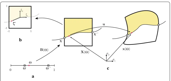
Fig. 4 Convective to local coordinates transformation. A point located atin the surface parametric space (a) is mapped to the reference configurationX() on the global coordinates system (c) and then to the local element space (b) with coordinatesζe
using a technique based on the work of Sevilla et al. [28]. With this procedure the points used for surface numerical integration are located over the actual CAD definition of the boundary (Fig.3c), and the volume subdomains account for the actual intersected volume in the element. Other specific methods to obtain the volume and surface subdomains and quadratures for particular cases, such as multiple surfaces within a boundary element, can be found in [5].
Convective to local coordinates transformation
It is worth to remark that for the case of a point lying on(i)the reference configuration
mapping is described using the surface convective coordinates, whereas the FE solution
uh is defined with the shape functions of the elements, which are independent of the
geometry. Figure4shows the coordinate transformations involved in the evaluation of the displacement field for a surface point with convective coordinates, whereB() represents the surface parametric transformation to the global space, X = B(). The reference and deformed configurations are shown in the Figure with coordinatesXand
x, and the reference element used to define the shape functionsN(ζe) is depicted on the left. As all the elements in cgFEM are regular hexahedrons the backward mapping from the global space to the local element spaceζeis straightforward. For a given point with coordinatesX=B() we have:
ζe= B()−Xe
h/2 (6)
where Xe is the center and h the size of the element. The partial derivatives of this
mapping with respect to the convective coordinates are involved in the kinematic variables definition and can be formulated as:
∂ζe
∂ξ = 2
hB,ξ;
∂ζe
∂η = 2
Variation of kinematic variables
In this work we use the exact variation ofx(1)andx(2), which ensures the symmetry of the formulation and the conservation of the angular momentum. Therefore the variation of the position vector for each body is formulated as:
δx(1)=x(1) ,u δu
δx(2)=x(2)
,ξ δξ+x(2),η δη+x,u(2)
δu (8)
The variationsδξandδηin Eq. (8) are obtained by projecting Eq. (4) intox,ξ(1)andx(1),η . Considering thatx(1),ξ ·n(1)=0,x,(1)η ·n(1)=0, the following system is presented:
x(2)
,ξ ·x,ξ(1)x(2),η ·x(1),ξ x(2)
,ξ ·x,η(1)x(2),η ·x(1),η
δξ δη
=
gNδn(1)·x(1),ξ −(x,u(2)−x(1),u)·x(1),ξ gNδn(1)·x(1),η −(x,u(2)−x(1),u)·x(1),η
(9)
where the last term to calculate is the variation of the normal gap. Starting from (3), the variation is evaluated as:
δn(1)=n(1) ,uδu
n(1) ,u =
x(1)
,u,ξ×x(1),η +x(1),ξ ×x,u,η(1)
nˆ(1) −
n(1) nˆ(1) n
(1)·(x(1)
,u,ξ×x,η(1)+x,(1)ξ ×x(1),u,η)
(10)
Surface definition using linear facets
Having the surface segments topology provided by the Marching Cubes algorithm we define a linear mappingBl() from the unit triangle to the segment in the initial
config-uration,X=Bl(). Therefore the position vector in the deformed configuration and its derivatives are defined as:
x=Bl()+N(ζe)u, x∈ c x,u=N(ζe)
x,ξ =Bl,ξ()+N,ζe(ζe)∂ζ e
∂ξ u
x,u,ξ =N,ζe(ζe)∂ζ e
∂ξ
x,ξ,ξ =N,ζe,ζe(ζe)∂ζ e
∂ξ ∂ζe
∂ξ u+N,ζe(ζe)∂
2ζe
∂ξ2u (11)
whereN(ζe),N,ζe(ζe) andN,ζe,ζe(ζe) are the FE shape functions and its respective
deriva-tives, andζeis evaluated as a function offrom (6). The partial derivatives with respect toηare evaluated similarly to the termsx,ξ,x,u,ξ andx,ξ,ξ. As the contact segments are linear, the tangent vectorsx,ξ,x,η(and consequently the normal vectorn(1)) are constant in a segment, and discontinuous between adjacent segments. This fact can produce a loss of convergence in the search of the contact active set, especially for coarse discretizations of the solids.
Surface definition using NURBS and FE displacements
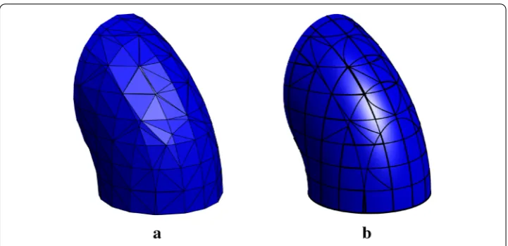
Fig. 5 Surface segments of a regular torus in cgFEM using the same approximation mesh.aLinear facets,b
NURBS surface segments
The surface and volume subdomains can be created considering the exact geometry of the domain (Fig.5), provided that it is defined by NURBS surfaces, which is nowadays a standard among the CAD industry. NURBS surfaces are rational functions defined in their own parametric space of coordinates (ξ,η) as
Q(ξ,η)=
n
i=1 m
j=1
Ni(p)(ξ)Mj(q)(η)wi,j
n
i=1
m
j=1N( p) i (ξ)M
(q) j (η)wi,j
Pi,j (12)
whereNi(p)andMj(q)are one-dimensional basis functions of orderpandqrespectively, each one defined along two knot vectors withnandmcontrol points.Pi,jare the
coordi-nates of then×mcontrol points of the surface. Equation (12) can be simplified for further developments as:
Q(ξ,η)=
n
i=1 m
j=1
Si,j(ξ,η)Pi,j (13)
where the termSi,j(ξ,η) is the NURBS basis function associated to the control point (i, j):
Si,j(ξ,η)=
Ni(p)(ξ)Mj(q)(η)wi,j
n
i=1
m
j=1N (p) i (ξ)M
(q) j (η)wi,j
(14)
We can carefully rearrange the indexation of the control points from (i, j) to the unique indexk, hence, we can rewrite the NURBS surface as a vector-matrix multiplication:
Q(ξ,η)=
n×m
k=1
Sk(ξ,η)Pk =S(ξ,η)·P (15)
where S(ξ,η) is a row vector containing then×mNURBS basis functions, andPis a (n×m)×3 matrix with the coordinates of all the control points of the surface. If we use the NURBS to define the reference configuration ofc(i)(1) and its derivatives are rewritten
Fig. 6 Example of NURBS fitting to the FE solution.aNURBS definition ofc.bFE solutionuh.cNURBS
fitting touh
x=Q(ξ,η)+N(ζe)u, x∈c x,u=N(ζe)
x,ξ =Q,ξ(ξ,η)+N,ζe(ζe)∂ζ e
∂ξ u
x,u,ξ =N,ζe(ζe)∂ζ e
∂ξ
x,ξ,ξ =Q,ξ,ξ(ξ,η)+N,ζe,ζe(ζe)∂ζ e
∂ξ ∂ζe
∂ξ u+N,ζe(ζe)∂
2ζe
∂ξ2u (16)
Differentiating (12) we can obtain the NURBS derivatives:
Q,ξ= ∂S∂ξ(ξ,η)P; Q,η= ∂S(ξ,η)
∂η P (17)
Displacement of the NURBS surface matching the FE solution
The last alternative is a step further in the use of NURBS surfaces to define the position of a point laying onc. Letube the FE displacements obtained for the current iteration
during the solution process. Then the following least squares problem is proposed to fit the contact surface (Eq. (15)) to the solutionuh:
min
1 2
(i)
c
(S(ξ,η)V−N(ζe)u)2dξdη
(18)
whereVare the displacements of control pointsPsuch as the NURBS surface matches the displacement field given by the FE solution. Figure6illustrates this idea with a simple example. The boundarycis represented in Fig.6a, with the control points net depicted
in red. Assuming the solutionuhevaluated over this surface is as in Fig.6b the NURBS
is fitted to that solution (Fig.6c). It is straightforward that the quality of this fitting will strongly depend on the “flexibility” of the surface, this is, the degree and number of knots of the NURBS. To overcome this issue there exist degree elevation and knot insertion algorithms which increase the degrees of freedom without changing the original surface.
The least squares problem in (18) can be solved using numerical integration overc:
V=M−1Gu (19)
where
M=
i
S(ξ,η)Ti S(ξ,η)i|J|iHi; G=
i
If the contact surface is modified such that the FE solution is implicitly included, the position of a given point ofccan be expressed using only the modified NURBS definition:
x=S(ξ,η) (P+V)=S(ξ,η) (P+Cu), x∈c (21)
with C = M−1G. Note that Cis a constant matrix which is defined for each different NURBS surface in(ci). These matrices can be calculated once previously and then used
during the solving algorithm saving computational cost. For this case the derivatives of the position vector are expressed as:
x,u=S(ξ,η)C
x,ξ =S,ξ(ξ,η) (P+Cu)
x,u,ξ =S,ξ(ξ,η)C
x,ξ,ξ =S,ξ,ξ(ξ,η) (P+Cu) (22) The evaluations of the position vector and all its derivatives becomes considerably easier thanks to the use of a unique NURBS in comparison with a mixed definition using the NURBS and the FE solution. The intersection procedure is also faster, since only surface evaluations must be computed. However, matrixCcouples all the elements in the mesh that contain the same surface, making this method non-viable in terms of computational cost for refined meshes.
Note that in both proposed alternatives the NURBS surface is implicitly considered through the numerical integration, and in the last one the nodes of the Cartesian grid are coupled with the control points of the contact NURBS through the gap definition. However, no additional degrees of freedom are included over the boundary and, in contrast with NURBS-enriched contact formulations as [24], the standard FE interpolation is kept inside the domain.
Stabilized Lagrangian contact formulation
This study is focused on the solution of frictionless 3D contact problems using the cgFEM, so we recall the stabilized Lagrange functional presented in [7]. The solution of the contact problem is the displacement fielduand the Lagrange multipliers fieldλN that optimizes
the following stabilized Lagrangian:
opt
(u)+ 1 2κ1
(1)
c
λN +κ1gN
2
−− |λN|2
d− 1
2κ2
(1)
c
(λN−pN)2d
(23)
with (u) containing all the terms related to the finite strain elasticity,κ1,κ2are penalty
constants, and we use the negative part operator which is defined as:
[x]−= ⎧ ⎪ ⎨ ⎪ ⎩
−x if x≤0
0 if x>0
(24)
We introduce the normal stabilizing stresspN =n(1)·σ∗·n(1), whereσ∗is a smooth
technique [12,13]. This term is considered independent of the solution, and an external loop is introduced to re-evaluate it. We experienced that the number of iterations is usually only between 2-4. Taking variations in Eq. (23) we can assume thatσ∗is constant and we obtain the following system:
⎧ ⎪ ⎪ ⎪ ⎪ ⎨ ⎪ ⎪ ⎪ ⎪ ⎩
δ (u,δu)−
(1)
c
λN +κ1gN
−δgN d=0, ∀δu
− 1 κ1 (1) c
λN+κ1gN
−+λN
δλNd−
1 κ2
(1)
c
(λN −pN)δλNd=0, ∀δλN
(25)
The Lagrange multipliers in the second Equation in (25) can be condensed element-wise [7] when considering the numerical integration, obtaining the following result:
λN g =
⎧ ⎪ ⎪ ⎨ ⎪ ⎪ ⎩
κ2gN g+pN g if
λN g+κ1gN g
≤0
0 if
λN g+κ1gN g
>0
(26)
This is defined for each quadrature point depicted by sub-indexg. The substitution ofλN
in the numerical integration of (25) yields the following equation: δ (u,δu)−gpN g+ κEhgN gδgN g|J|gHg =0, if
pN g+κhEgN g≤0 δ (u,δu)=0, if
pN g+κhEgN g
>0
(27)
where κhE =(κ1+κ2) is the penalty term,Eis the elastic modulus,his the mesh size,Hg
is the quadrature weight and,|J|gis the Jacobian of the transformation.
Linearization of kinematic variables
The formulation used above is solved using the Newton-Raphson method, therefore, the linearizations of the kinematic variables in Eq. (27), i.e.,gN andδgN are needed. The
same process performed in (5) can be used to obtaingN. For the linearizationδgNwe
start from (4) and obtain the following expression: δx(2)(ξ,η)=δg
Nn(1)+δgNn(1)+gNδn(1)+gNδn(1)+δx(1) (28)
which, after multiplying byn(1), results in:
δgN =
δx(2)(ξ,η)−δx(1)·n(1)−g
Nδn(1)·n(1) (29)
We can now obtain the linearizationsδx(1),δx(2)from Eq. (8): δx(2)=δu x(2)
,ξ,ξξδξ+x(2),η,ηηδη+x(2),ξ,η(ξδη+δξη)+x,u,ξ(2)δξ+
+x(2)
,u,ξξ+x,u,η(2)δη+x(2),u,ηη+x(2),ξ δξ+x,η(2)δη
u
δx(1)=0 (30)
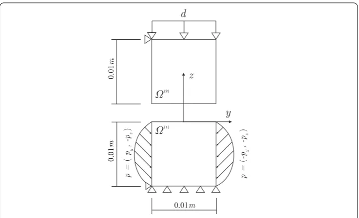
Fig. 7 Example 1. Contact between plane surfaces. Sketch of problem
Numerical examples Contact between plane surfaces
In this example, similar to [29,30], a simple analysis of contact between plane surfaces is solved to test the convergence of the FE solution using the different surface definitions described in this paper. The 2D sketch of the solids in contact is depicted in Fig.7, where
x is the out-of-plane direction. Both solids have common elastic material properties,
E =115GPa andν=0.3. At the initial configuration, the contact surfaces are overlapping and vertical displacementd = −1.6×10⁻⁶m is applied on the upper face of the upper body. Displacements alongydirection are constrained on the upper face of body 2 and on the lower face of body 1. We use a 2D plane strain overkill solution from [30] as a reference for the discretization error evaluation, so symmetry conditions are applied to the faces parallel to theyzplane. The lateral faces of body 1 are loaded withpy=4·1011(0.01−z)z Pa
andpz=10·1011(0.01−z)z Pa.
Non-conforming Cartesian grids are used on both bodies. Figure8shows some of the uniformly refined meshes used for the analysis. Starting with the first discretization in Fig.
8each element is subdivided into 8 new elements to build the following mesh.
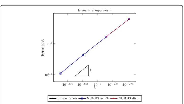
The convergence of the relative error in energy norm is shown in Fig.9for a sequence of 4 meshes using linear elements,H8. The results show that, for all the surface definitions,
optimal convergence rate of the error in energy norm (represented by the triangle) is achieved. Only two meshes were solved with the fitting NURBS definition due to the high amounts of nodes coupled in the following meshes.
Fig. 8 Example 1. Refinement process for the study of the convergence of the solution. Meshes 1 to 3 are shown from left to right
10−3.4 10−3.2 10−3 10−2.8 10−2.6 100.5
101
1
h
E
rr
o
ri
n%
Error in energy norm
Linear facets NURBS + FE NURBS disp.
Fig. 9 Example 1: Evolution of the error in energy norm with the element size of the lower body. Convergence of the FE solution
When the contact occurs between planar surfaces there is practically no difference in the definition of the surfaces using the three presented methods, and the gap measurement is trivial. Therefore, as expected, all methods have results with a similar precision.
Contact between curved surfaces, finite deformations
The second example considers the contact interaction between elastic solids with a toroidal shape with major radiusR=2 cm and minor radiusr=0.5 cm. Figure11shows the initial position of the bodies in contact. A positive displacement is imposed along the
ydirection over the purple surfaces in 5 incremental steps of 0.1cm. All the DOFs are constrained over the blue surfaces. A Neo-Hookean material is used withE = 116GPa
andν=0.3.
0 0.2 0.4 0.6 0.8 1
·10−2
−2
−1.8
−1.6
−1.4
−1.2
·10−6
y(m)
uz
(
m
)
Displacements at the contact surface
Linear facetsuh NURBSuh NURBS fitting
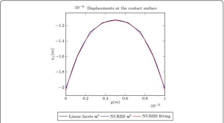
Fig. 10 Example 1: FE displacementsuhover the top surface of the lower solid considering linear facets and
NURBS fitting definitions. The curve in red depicts the solution of the NURBS fitting problem
Fig. 11 Example 2. Contact simulation between curved surfaces. A positive displacement along they direction is imposed over the purple surfaces. All the DOFs are constrained over the blue surfaces
for one of the solids. No results were obtained when using linear facets with the first of the meshes due to loss of convergence caused by the surface discretization being extremely coarse. However, the same coarse mesh had no convergence problems using the other two surface definitions, thanks to the consideration of the exact geometry. The last mesh was not solved using the NURBS displacement method due to the high amount of nodes coupled by each surface, which results in non-viable computational cost.
Fig. 12 Example 2. Refinement process for the analysis of contact between curved surfaces. Meshes 1 to 3 are shown from left to right. Both solids are meshed with a similar discretization.a216 nodes.b1052 nodes.c
5268 nodes
1 2 3 4 5
1 2 3 4 5
·109
Load step number
Reaction
forces
(
N
)
Reaction Forces
NURBS+FE, mesh 1 NURBS+FE, mesh 2 NURBS+FE, mesh 3 Linear facets, mesh 2 Linear facets, mesh 3 NURBS disp., mesh 1
NURBS disp., mesh 2
Fig. 13 Example 2. Reaction forces on the Dirichlet constrained surfaces during the load
including the results obtained with NURBS+FE and NURBS fitting for the coarse mesh. This is mainly due to the lower precision in the gap measurement with linear facets.
The values ofσyat the final load step for all the performed analyses is shown in Fig. 14. The results are similar for the different methods, with the maximum stress value increasing with the refinement of the mesh.
Fig. 14 Example 2. Values ofσy(Pa) at final load step for all the analyses. *The image inashows the coarse surface discretization which led to loss of convergence.aLinear, mesh 1*.bLinear, mesh 2.cLinear, mesh 3.d
Fig. 15 Example 2. Finite deformations with Neo-Hookean material. Deformed shape usingaLinear facets,b
NURBS + FE solution. The color map represents values ofuh.cSurface integration points with active contact
Fig. 16 Example 3. Small deformations contact between curved surfaces. A positive displacement along the ydirection is imposed over the purple surfaces. All the DOFs are constrained over the blue surfaces
Contact between curved surfaces, small deformations
The last example consists in a small deformations contact simulation between three torus. The geometric parameters are the same as in the previous example. For this problem a linear elastic material has been considered, withE=115 GPa andν=0.3, and only one increment of 0.05cmhas been applied in theydirection over the purple surfaces, shown in Fig.16. The problem was solved using linear facets and NURBS + FE definition, with the meshes in Fig.12a, b respectively.
Fig. 17 Example 3. Small deformations contact between three torus. Von Mises stress for the central torus (Pa) with exact geometry consideration and linear facets.aFacets, 216 nodes.bFacets, 1052 nodes
Conclusions
Three different alternatives have been presented to define the contact surfaces within the Cartesian grid finite element method: a linear facet representation, a combination of NURBS surface and FE displacements and the fitting of a NURBS surface to the FE displacements. The first option, is the most simple and fastest of all three in terms of procedure and implementation. The surface integration quadratures are based on linear triangles whose rules are well known. The ray-tracing algorithm becomes a linear equa-tion, thus having an analytical solution. Therefore the gap is easily computed. In terms of implementation, the normal vector is constant along a surface subdomain (triangle) reducing the number of terms in the calculation of the kinematic variables. On the other hand, this method has lower precision in the gap measure, which can affect the robustness of the method, specially with coarse discretizations.
The use of NURBS surfaces combined with FE solution provides with better results compared with linear facets, as the actual CAD geometry is considered regardless of the used discretization. In all the tests analysed the precision of the solution computed in terms of energy error or stresses is always greater or equal than that obtained with linear facets. This is specially true for coarse discretizations, due to the enhanced gap measure. Some drawbacks of this method are related to the computational cost of the quadrature rules creation [5] and the solution of the ray-tracing algorithm (non-linear equation). In terms of implementation, more terms are involved in the evaluation of the kinematic variables and its variations. However, the total computational cost is not compromised, as the results obtained with NURBS surfaces and coarse meshes have a similar quality as those obtained with finer meshes and linear facets.
the high coupling of degrees of freedom for fine discretizations should be addressed, as the computational cost grows exponentially. For these reasons, the combination of NURBS and FE solution seems to be the most versatile and robust option to define the contact surfaces in the framework of the cgFEM.
Authors’ contributions
MT carried out the theoretical developments and supervised the implementation. JMN implemented the developments, collected data and drafted the manuscript. MT, JJR and FJF revised the manuscript. All authors read and approved the final manuscript.
Acknowledgements
The authors wish to thank the Spanish Ministerio de Economia y Competitividad the Generalitat Valenciana and the Universitat Politècnica de València for their financial support received through the projects DPI2017-89816-R, Prometeo 2016/007 and the FPI2015 program.
Competing interests
The authors declare that they have no competing interests.
Availability of data and materials
Not applicable.
Ethics approval and consent to participate
Not applicable.
Funding
Funded by Spanish Ministerio de Economia y Competitividad (project DPI2017-89816-R), Generalitat Valenciana (project Prometeo 2016/007) and Universitat Politècnica de València (program FPI2015).
Publisher’s Note
Springer Nature remains neutral with regard to jurisdictional claims in published maps and institutional affiliations.
Received: 2 January 2018 Accepted: 3 May 2018
References
1. Düster a, Parvizian J, Yang Z, Rank E. The finite cell method for three-dimensional problems of solid mechanics. Comput Methods Appl Mech Eng. 2008;197(45–48):3768–82.https://doi.org/10.1016/j.cma.2008.02.036. 2. Schillinger D, Ruess M. The finite cell method: a review in the context of higher-order structural analysis of CAD and
image-based geometric models. Arch Comput Methods Eng. 2015;22(3):391–455.https://doi.org/10.1007/ s11831-014-9115-y.
3. Burman E, Claus S, Hansbo P, Larson MG, Massing A. CutFEM: discretizing geometry and partial differential equations. Int J Numer Methods Eng. 2015;104(7):472–501.https://doi.org/10.1002/nme.4823.
4. Nadal E, Ródenas JJ, Albelda J, Tur M, Tarancón JE, Fuenmayor FJ. Efficient finite element methodology based on cartesian grids: application to structural shape optimization. Abstr Appl Anal. 2013;2013:1–19.https://doi.org/10. 1155/2013/953786.
5. Marco O, Sevilla R, Zhang Y, Ródenas JJ, Tur M. Exact 3D boundary representation in finite element analysis based on Cartesian grids independent of the geometry. Int J Numer Methods Eng. 2015;103(6):445–68.https://doi.org/10. 1002/nme.4914.
6. Tur M, Albelda J, Marco O, Ródenas JJ. Stabilized method of imposing Dirichlet boundary conditions using a recovered stress field. Comput Methods Appl Mech Eng. 2015;296:352–75.https://doi.org/10.1016/j.cma.2015.08. 001.
7. Tur M, Albelda J, Navarro-Jimenez JM, Rodenas JJ. A modified perturbed Lagrangian formulation for contact problems. Comput Mech. 2015;55(4):737–54.https://doi.org/10.1007/s00466-015-1133-6.
8. Heintz P, Hansbo P. Stabilized Lagrange multiplier methods for bilateral elastic contact with friction. Comput Methods Appl Mech Eng. 2006;195(33–36):4323–33.https://doi.org/10.1016/j.cma.2005.09.008.
9. Annavarapu C, Hautefeuille M, Dolbow JE. A Nitsche stabilized finite element method for frictional sliding on embedded interfaces. Part I: single interface. Comput Methods Appl Mech Eng. 2014;268:417–36.https://doi.org/10. 1016/j.cma.2013.09.002.
10. Poulios K, Renard Y. An unconstrained integral approximation of large sliding frictional contact between deformable solids. Comput Struct. 2015;153:75–90.https://doi.org/10.1016/j.compstruc.2015.02.027.
11. Mlika R, Renard Y, Chouly F. An unbiased Nitsche’s formulation of large deformation frictional contact and self-contact. Comput Methods Appl Mech Eng. 2017;325:265–88.https://doi.org/10.1016/J.CMA.2017.07.015. 12. Zienkiewicz OC, Zhu JZ. The superconvergent patch recovery and a posteriori error estimates. Part 1: the recovery
13. Ródenas JJ, Tur M, Fuenmayor FJ, Vercher A. Improvement of the superconvergent patch recovery technique by the use of constraint equations: The SPR-C technique. Int J Numer Methods Eng. 2007;70:705–27.https://doi.org/10. 1002/nme.1903.
14. González-Estrada OA, Ródenas JJ, Bordas SPA, Nadal E, Kerfriden P, Fuenmayor FJ. Locally equilibrated stress recovery for goal oriented error estimation in the extended finite element method. Comput Struct. 2015;152:1–10. https://doi.org/10.1016/j.compstruc.2015.01.015.
15. Wriggers P, Krstulovic-Opara L, Korelc J. Smooth c1-interpolations for two-dimensional frictional contact problems. Int J Numer Methods Eng. 2001;51(12):1469–95.https://doi.org/10.1002/nme.227.
16. Padmanabhan V, Laursen TA. A framework for development of surface smoothing procedures in large deformation frictional contact analysis. Finite Elem Anal Design. 2001;37(3):173–98.https://doi.org/10.1016/
S0168-874X(00)00029-9.
17. Tur M, Giner E, Fuenmayor FJ, Wriggers P. 2d contact smooth formulation based on the mortar method. Comput Methods Appl Mech Eng. 2012;247–248:1–14.https://doi.org/10.1016/j.cma.2012.08.002.
18. Stadler M, Holzapfel GA, Korelc J. Cn continuous modelling of smooth contact surfaces using NURBS and application to 2D problems. Int J Numer Methods Eng. 2003;57(15):2177–203.https://doi.org/10.1002/nme.776.
19. Puso MA, Laursen TA. A 3d contact smoothing method using gregory patches. Int J Numer Methods Eng. 2002;54(8):1161–94.https://doi.org/10.1002/nme.466.
20. Neto DM, Oliveira MC, Menezes LF, Alves JL. A contact smoothing method for arbitrary surface meshes using nagata patches. Comput Methods Appl Mech Eng. 2016;299:283–315.https://doi.org/10.1016/j.cma.2015.11.011. 21. Hughes TJR, Cottrell Ja, Bazilevs Y. Isogeometric analysis: CAD, finite elements, NURBS, exact geometry and mesh
refinement. Comput Methods Appl Mech Eng. 2005;194(39–41):4135–95.https://doi.org/10.1016/j.cma.2004.10.008. 22. De Lorenzis L, Wriggers P, Hughes TJR. Isogeometric contact: a review. GAMM-Mitteilungen. 2014;37(1):85–123.
https://doi.org/10.1002/gamm.201410005.
23. Dittmann M, Franke M, Temizer I, Hesch C. Isogeometric analysis and thermomechanical mortar contact problems. Comput Methods Appl Mech Eng. 2014;274:192–212.https://doi.org/10.1016/j.cma.2014.02.012.
24. Corbett CJ, Sauer RA. NURBS-enriched contact finite elements. Comput Methods Appl Mech Eng. 2014;275:55–75. https://doi.org/10.1016/J.CMA.2014.02.019.
25. Corbett CJ, Sauer RA. Three-dimensional isogeometrically enriched finite elements for frictional contact and mixed-mode debonding. Comput Methods Appl Mech Eng. 2015;284:781–806.https://doi.org/10.1016/j.cma.2014. 10.025.
26. Navarro-Jiménez JM, Tur M, Albelda J, Ródenas JJ. Large deformation frictional contact analysis with immersed boundary method. Computational Mechanics. 2018; 1–18.https://doi.org/10.1007/s00466-017-1533-x.
27. Lorensen WE, Cline HE, Lorensen WE, Cline HE. Marching cubes: a high resolution 3D surface construction algorithm. In: Proceedings of the 14th annual conference on computer graphics and interactive techniques—SIGGRAPH ’87, vol. 21. 1987. p. 163–169. New York: ACM Press.https://doi.org/10.1145/37401.37422.http://portal.acm.org/citation. cfm?doid=37401.37422.
28. Sevilla R, Fernández-Méndez S, Huerta A. NURBS-enhanced finite element method (NEFEM). Int J Numer Methods Eng. 2008;76:56–83.https://doi.org/10.1002/nme.2311.
29. Hüeber S, Mair M, Wohlmuth BI. A priori error estimates and an inexact primal-dual active set strategy for linear and quadratic finite elements applied to multibody contact problems. Appl Numer Math. 2005;54(3–4):555–76.https:// doi.org/10.1016/J.APNUM.2004.09.019.