R E S E A R C H A R T I C L E
Open Access
Explicit Verlet time-integration for a
Nitsche-based approximation of
elastodynamic contact problems
Franz Chouly
1and Yves Renard
2**Correspondence: [email protected] 2ICJ UMR5208, LaMCoS UMR5259, Université de Lyon, INSA-Lyon, 20 rue Albert Einstein, 69621 Villeurbanne, France Full list of author information is available at the end of the article
Abstract
The aim of the present paper is to study theoretically and numerically the Verlet scheme for the explicit time-integration of elastodynamic problems with a contact condition approximated by Nitsche’s method. This is a continuation of papers (Chouly et al. ESAIM Math Model Numer Anal 49(2), 481–502,2015; Chouly et al. ESAIM Math Model Numer Anal 49(2), 503–528,2015) where some implicit schemes (theta-scheme, Newmark and a new hybrid scheme) were proposed and proved to be well-posed and stable under appropriate conditions. A theoretical study of stability is carried out and then illustrated with both numerical experiments and numerical comparison to other existing discretizations of contact problems.
Keywords: Unilateral contact, Elastodynamics, Nitsche’s method, Explicit time-marching schemes, Stability, Explicit dynamics
Introduction and problem setting
Explicit time-marching schemes for the dynamics of deformable solids with impact has already been the subject of an abundant literature (see, e.g., [1–3] for some recent con-tributions). They are appealing since they can be easy to implement, fast and adapted to parallel architectures. Nevertheless, there still remains important difficulties to design robust explicit methods and to obtain reliable numerical simulations in this context (see, e.g., [4]). Among these difficulties, numerical stability and energy conservation remains one of the most important ones. Another one is to preserve the quality and the accuracy of the numerical solution, which can present spurious oscillations in the displacement, the velocity or the contact stress. A last one is to enforce properly the contact condition, particularly the non-penetration condition.
A precursory method is the one developed by Taylor and Flanagan [5] in the framework of PRONTO3D software (see also the description in [6]). Nevertheless, the method is not fully explicit, except in a node-to-node contact approximation, in the sense that the contact pressure is computed in an iterative process on the whole contact surface. To mention some other of the most important contributions, we can say that a widely resumed theoretical work in dynamic impact problems is due to Moreau [7,8] for the impact of rigid body systems. The (implicit) schemes proposed by Moreau have been extended quite naturally to the elasticity case through finite element semi-discretization
©The Author(s) 2018. This article is distributed under the terms of the Creative Commons Attribution 4.0 International License (http://creativecommons.org/licenses/by/4.0/), which permits unrestricted use, distribution, and reproduction in any medium, provided you give appropriate credit to the original author(s) and the source, provide a link to the Creative Commons license, and indicate if changes were made.
in space (for instance in [9]) which transforms the continuous impact problem into a discrete one very close to a rigid body system. These discrete impact problems, governed by a so-called measure differential inclusion are notoriously ill-posed and of very low regularity.
The ill-posedness can be fixed (for the most part) by the addition of an impact law with a restitution coefficient. As a matter of fact, standard schemes, such as the commonly used ones of Newmark’s family [10], have an erratic behavior when they are applied to dynamic contact problems. This is mainly because they select a solution corresponding to an arbitrary (and potentially very large) restitution coefficient (see [11]). Alternatively, a valuable scheme in this context is that of Paoli and Schatzman [12,13] who implicitly takes into account this restitution coefficient. However, the addition of a restitution coefficient can be considered as artificial in the context of deformable solids. This does not diminish the interest for the Paoli–Schatzman scheme which will be a point of comparison with our proposed approach. The implicit inclusion of a restitution coefficient has also been considered in [14] to develop a wide range of schemes based on a time discontinuous Galerkin framework.
As noticed in [11], even in the case where the continuous problem is well-posed (see, e.g., [15,16] for well-posedness results), the ill-posed measure differential inclusion that results from finite element semi-discretization in space has an infinite number of solutions, depending on the choice of a restitution coefficient on each node of the contact boundary. Moreover, it is not possible to decide which solution is more suitable than other. Indeed, the two most remarkable solutions are, on the one hand, the one for a unitary restitution coefficient which ensures conserving energy but which causes very important spurious oscillations of the contact nodes and unexploitable contact stress, and, on the other hand, the solution for a vanishing restitution coefficient which ensures stability and a better approximation of the contact stress but is energy dissipative, while the continuous problem is not. This resulted in [11] to design the mass redistribution method (generalized in [17,18]) which allows a compromise in this context, i.e. well-posedness of the space semi-discretized problem, conservation of the energy and an improved quality of the contact stress. However, and this is also the case for the Paoli–Schatzman scheme, it introduces a global problem to be solved (at least on the contact nodes) when an explicit time-marching scheme is used. In the same spirit, a time-marching scheme has been designed in [19] for dynamic fracture problems, in which the cohesive forces are treated implicitly, while an explicit scheme is used for the dynamics of interior nodes.
prob-lem, and more robust with respect to the Nitsche parameter. Nitsche’s method, orig-inally designed to enforce weakly Dirichlet boundary conditions [23,24], was adapted to unilateral contact in [25,26] (see also [27] for an overview of recent results on this topic).
We studied previously in [28,29] the behavior of Nitsche’s method for contact in elastodynamics, when combined to various implicit time-marching schemes. Particu-larly, when applied to contact-impact in elastodynamics, Nitsche’s method has the good property of leading to a well-posed semi-discrete problem in time (i.e., a system of Lipschitz differential equations) as it is shown in [28]. This feature is shared also by the penalty method and modified mass methods. Moreover the symmetric variant of Nitsche’s space semi-discretization conserves an augmented energy [28], as does the penalty method [30]. We studied as well theoretically the well-posedness, the stabil-ity and energy conservation properties of fully discrete schemes based on space semi-discretization with Nitsche’s method combined with the theta-scheme, the Newmark scheme and a new Hybrid scheme. This study was illustrated with some numerical exper-iments.
The aim of this paper is to study mathematically and numerically the approximation of contact problems in elastodynamics by Nitsche’s method combined with the explicit Verlet time-marching scheme. The choice of the Verlet scheme is motivated both by its simplicity and its attractive theoretical properties (symplecticity) [31]. We will also make comparisons with some of the existing methods mentioned above and with the approximation by penalized contact. The numerical comparison will be mainly performed on the one-dimensional problem introduced in [15] whose advantage is to present a known periodic solution and to make clear the occurrence of parasitic oscillations, the convergence and energy conservation properties. Comparisons for 2D and 3D problems will also be presented.
Let us introduce some useful notations. In what follows, bold letters likeu,v, indicate vector or tensor valued quantities, while the capital ones (e.g.,V,K. . .) represent func-tional sets involving vector fields. As usual, we denote by (Hs(.))d,s ∈R, d= 1,2,3 the Sobolev spaces in one, two or three space dimensions (see [32]). The usual scalar product of (Hs(D))dis denoted by (·,·)
s,Dand the corresponding norm is denoted by · s,D—we keep the same notation whend=1 ord>1. The letterCstands for a generic constant, independent of the discretization parameters.
We consider an elastic body inRd with d = 1,2,3. Small strain assumptions are
made (as well as plane strain whend =2). The boundary∂ofis polygonal (d =2)
or polyhedral (d=3). The normal unit outward vector on∂is denotedn. We suppose that∂consists in three nonoverlapping partsD,Nand the contact boundaryC, with meas(D)>0 and meas(C)>0. In its initial stage, the body is in contact onC with a rigid foundation and we suppose that the unknown contact zone during deformation is included intoC. The body is clamped onDfor the sake of simplicity. It is subjected to volume forcesfinand to surface loadsgonN.
ρu¨−divσ(u)=f, σ(u)=Aε(u) inT,
u=0 onDT,
σ(u)n=g onNT,
u(0,·)=u0 u˙(0,·)=u˙0 in,
(1)
where the notation ˙xis used for the time-derivative of a vector fieldxonT, so that ˙uis the velocity of the elastic body and ¨uits acceleration;u0and ˙u0are initial displacement
and velocity. The density of the elastic material is denoted byρ, and is supposed to be a constant to simplify the presentation (this is not restrictive and the results can be extended straightforwardly for a variable density). The notationσ= (σij), 1≤i, j≤d,stands for the stress tensor field anddivdenotes the divergence operator of tensor valued functions. The notationε(v) = (∇v+∇vT)/2 represents the linearized strain tensor field andA is the fourth order symmetric elasticity tensor having the usual uniform ellipticity and boundedness property. For any displacement fieldvand for any density of surface forces σ(v)ndefined on∂we adopt the following notation
v=vnn+vt and σ(v)n=σn(v)n+σt(v),
where vt (resp. σt(v)) is the tangential component ofv (resp. σ(v)n). The conditions
describing unilateral contact without friction onCTare:
un≤0 σn(u)≤0 σn(u)un=0 σt(u)=0. (2)
Note additionally that the initial displacementu0should satisfy the compatibility
Condi-tionu0n≤0 onC.
To our knowledge, the well-posedness of Problems (1), (2) is still an open issue. The few available existence results concern simplified model problems involving the (scalar) wave equation with Signorini’s conditions (see, e.g., [16,33–36]) or thin structures like membranes, beams (see [37]) or plates (see [38]). Even in these simplified cases, obtaining uniqueness and energy conservation still involves difficulties in 2D or 3D. For a review on some of these results, one can refer to the book [39].
We introduce the Hilbert space
V:=v∈H1()d :v=0onD
,
and the following forms:
a(u,v) :=
σ(u) :ε(v)d, L(t)(v) :=
f(t)·vd+
N
g(t)·vd,
for anyuandvinV, for allt∈[0, T]. The (total) mechanical energy associated with the solutionuof the dynamic contact problem (1,2) is:
E(t) := 1 2ρu˙(t)
2 0,+
1
2a(u(t),u(t)), ∀t∈[0, T].
Let us taket ∈[0, T]. Formally, we get from (1), after multiplication by ˙u(t), integration by parts, with the boundary conditions onDT,NTand the absence of friction:
u¨(t)·u˙(t)d+
σ(u(t)) :ε(˙u(t))d
d dtE(t)
−
C
Moreover, if we assume that the contact force does not dissipate any energy, i.e. satisfies the so called persistency Conditionσn(u(t))˙un(t)=0 (see, e.g., [30,40,41]) then we end up with:
d
dtE(t)=L(t)(˙u(t)). (3)
Notably, whenLvanishes, we get energy conservation:E(t)=E(0), for allt∈[0, T]. Note that, even if it is expected that solutions to Problems (1), (2) satisfy the persistency Condition σn(u(t))˙un(t) = 0 in order to respect the non-dissipative character of the frictionless contact condition, it has only been rigorously proved in a one dimensional framework (elastic bar) for instance in [36, Lemma 2.5].
The rest of our paper is outlined as follows. The first section is dedicated to the descrip-tion of the fully discrete formuladescrip-tion for dynamic contact with Nitsche and Verlet explicit time-integration. Then, a stability analysis is carried out, and finally, some numerical comparisons with other classical methods are investigated and analysed.
Discrete setting: Nitsche’s method with Verlet scheme
We begin this section with preliminary notations and results. Then, we introduce our Nitsche-based finite element semi-discretization in space, and we recall its main proper-ties of well-posedness and energy conservation. Finally we describe the fully discretized problem based on the Verlet explicit time-marching scheme.
Preliminary notations and results
We make use of the notation [·]R−, that stands for the projection onto R− ([x]R− = 1
2(x − |x|) for x ∈ R). The notation H(·) will stand for the Heaviside function
H(x)=1 ifx>0,12ifx=0, and 0 ifx<0, which satisfiesH(x)+H(−x)=1,∀x∈ R. Moreover we will make use of the equality H(−x)[x]R− = [x]R−, ∀x ∈ R, and the following property of projection:
(y−x)(y
R− −[x]R−)≥(
y
R−−[x]R−)
2 ∀x, y∈R. (4)
Let Vh ⊂ V be a family of finite dimensional vector spaces (see [42]) indexed by h coming from a familyThof triangulations of the domain(h=maxK∈ThhK wherehK is the diameter of the triangleK). The family of triangulations is supposed:
• Regular, i.e., there existsσ >0 such that∀K ∈ Th, hK/ρK ≤ σ whereρK denotes the radius of the inscribed ball inK,
• Conformal to the subdivision of the boundary intoD, N andC, which means
that a face of an elementK ∈ This not allowed to have simultaneous non-empty intersection with more than one part of the subdivision,
• Quasi-uniform, i.e., there existsc>0, such that,∀h>0, ∀K ∈Th, h K ≥ch.
To fix ideas, we choose a standard Lagrange finite element method of degreekwithk =1 ork=2, i.e.:
Vh=
vh∈(C0())d:vh|K ∈(Pk(K))d,∀K∈Th,vh=0onD
.
We consider in what followsγh, a positive piecewise constant function on the contact interfaceC which satisfies for everyK that has a non-empty intersection of dimension d−1 withC
γh|K∩C = γ0
hK
, (5)
whereγ0is a positive given constant (the Nitsche parameter). Note that the value ofγh on element intersections has no influence.
We next define convenient mesh-dependent norms, in fact weighted L2(
C)-norm (since (γ0/γh)|K =hK).
Definition 1 For anyv∈L2(C), we set
v−1
2,h,C := (γ0/γh) 1 2v0,
C, v1
2,h,C := (γh/γ0) 1 2 v0,
C.
Additionally, it will be convenient to endowVhwith the following mesh- and parameter-dependent scalar product:
Definition 2 For allvh,wh∈Vhwe set
(vh,wh)γh :=(vh,wh)1,+(γh
1
2vnh,γh12whn)0, C,
and note · γh :=(·,·)
1 2
γhthe corresponding norm. Remark that the two norms · γhand · 1,are equivalent onVh, in the following sense (for a quasi-uniform meshTh):
vh1,≤ vhγh ≤
1+Cγ0 h
1 2
vh1,,
for anyvh∈Vh. The positive constantCcomes from the trace inequality and the constant of quasi-uniformity of the meshTh. For a meshThthat is not quasi-uniform, the same relationship holds, replacinghby (minK∈ThhK).
We end this section with the following statement: a discrete trace inequality (see, e.g., [43]), that is a key ingredient for the whole mathematical analysis of Nitsche’s based methods.
Lemma 3 There exists C > 0, independent of the parameterγ0and of the mesh size h,
such that, for allvh∈Vh
σn(vh)−1
2,h,C ≤Cv
h
1,. (6)
Semi-discrete problem in space
Our Nitsche-based discretization of the contact condition comes from the following result (see [44] and as well [25] for a detailed formal proof).
Proposition 4 Letγ be a positive function defined onC. The contact Condition(2)can be reformulated as follows:
σn(u)=[σn(u)−γun]R−. (7)
Pn,γ h:
Vh→ L2(
C)
vh →σn(vh)−γhvhn .
Define as well the bilinear form:
Anγh(uh,vh) :=a(uh,vh)−
C γh σn
(uh)σn(vh)d.
The space semi-discretized Nitsche-based method for unilateral contact problems in elas-todynamics then reads (see, e.g, [27,28]):
⎧ ⎪ ⎪ ⎪ ⎪ ⎪ ⎪ ⎪ ⎨ ⎪ ⎪ ⎪ ⎪ ⎪ ⎪ ⎪ ⎩
Finduh: [0, T]→Vhsuch that fort∈[0, T]:
(ρu¨h(t),vh)0,+Anγh(uh(t),vh)+
C 1 γh
[Pn1,γh(uh(t))]R−Pn,γh(v
h)d
=L(t)(vh), ∀vh∈Vh, uh(0,·)=uh0, u˙h(0,·)=u˙h0,
(8)
where uh0 (resp. ˙uh0) is an approximation inVh of the initial displacementu0(resp. the
initial velocity ˙u0), for instance the Lagrange interpolant or theL2() projection ofu0
(resp. ˙u0).
Remark 5 Note that, as in [27], we adopted in this presentation a different convention for notations compared to previous works [28,29]. This is in order to get closer to the formulations provided in most of the papers on Nitsche’s method and on the augmented Lagrangian method.
We can reformulate (8) as a system of (non-linear) second-order differential equa-tions. To this purpose, using Riesz’s representation theorem in (Vh,(·,·)γh) we first intro-duce the mass operator Mh : Vh → Vh, which is defined for all vh,wh ∈ Vh by (Mhvh,wh)γh = (ρvh,wh)0,.Still using Riesz’s representation theorem, we define the (non-linear) operatorBh:Vh→Vh, by means of the formula
(Bhvh,wh)γh:=Anγ h(v
h,wh)+
C 1 γh
[Pn1,γ h(v
h)]
R−Pn,γh(w
h)d,
for allvh,wh∈Vh. Finally, we denote byLh(t) the vector inVhsuch that, for allt∈[0, T] and for everywhinVh: (Lh(t),wh)γh = L(t)(wh).With the above notation, Problem (8) reads: ⎧ ⎪ ⎪ ⎨ ⎪ ⎪ ⎩
Finduh: [0, T]→Vhsuch that fort∈[0, T]:
Mhu¨h(t)+Bhuh(t)=Lh(t),
uh(0,·)=uh0, u˙h(0,·)=u˙h0.
(9)
Moreover, we recall the results of well-posedness and the energy estimate for the semi-discrete problem in space, that were established in [28]. First, the following theorem together with the boundedness of(Mh)−1γh[see [28] show that Problem (8) or equiva-lently Problem (9)] is well-posed.
Theorem 6 The operatorBhis Lipschitz-continuous in the following sense: there exists a constant C >0, independent of h,andγ0such that, for allvh1,vh2∈Vh:
Bhvh
1−Bhvh2γh≤C(1+γ−
1
As a consequence, for every value of∈ Randγ0 > 0, Problem(8)admits one unique
solutionuh ∈ C2([0, T],Vh).
Remark 7 Note that, conversely to the static case (see [25,26,45]) and the fully-discrete case there is no condition onγ0for the space (semi-)discretization, which remains
well-posed even ifγ0is arbitrarily small. However, this does not imply that the solution remains
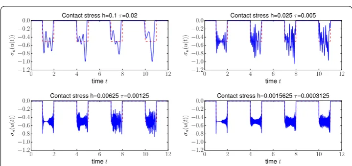
consistent whenγ0becomes small (see Remark19and Fig.4in the sequel).
We recall that the standard (mixed) finite element semi-discretization for elastodynam-ics with unilateral contact leads to ill-posed problems (see, e.g., [11,22]), which is not the case of Nitsche’s formulation that leads to a well-posed (Lipschitz) system of differen-tial equations. This feature is shared with the standard penalty method, the difference being that Nitsche’s method remains consistent in a strong sense (see [28]). Note that the standard (mixed) finite element semi-discretization is consistent as well as the singular dynamic method introduced in [18]. The mass redistribution method introduced in [11] is asymptotically consistent whenhvanishes.
Now, we consider the energy estimates which are counterparts of the Eq. (3), in the semi-discretized case. Let us define the discrete energy as follows:
Eh(t) := 1 2ρu˙
h(t)2
0,+ 12a(uh(t),uh(t)), ∀t∈[0, T].
which is associated to the solutionuh(t) to Problem (8). This is the direct transposition of the mechanical energyE(t) from the continuous system. As in [28], we define also a modified energy more suited to Nitsche’s method
Eh(t) :=Eh(t)− 2γ0
σn(uh(t))
2
−1 2,h,C
−[Pn1,γh(uh(t))]R−
2
−1 2,h,C
(11)
:=Eh(t)−Rh(t), (12)
in which a consistent term is added. This term denotedRh(t) represents, roughly speaking, the non-fulfillment of the contact Condition (7) byuh. The relationship betweenEh(t) andEh(t) is provided in the Lemma below:
Proposition 8 For≥0andγ0large enough, there exists C>0independent of h, ofγ0
and of the solution to Problem(8), such that, for all t∈[0, T]:
Eh(t)≤CEh(t).
Proof This result is obtained using the coercivity ofa(·,·) and applying Lemma3.
Remark 9 Proposition8states that the energyEh(t) remains always positive (ifEh(0) is) for≥0 andγ0large enough. Forγ0small, the existence of zero energy spurious modes
cannot be excluded.
Remark 10 For <0, such a result with a constant independent of the mesh parameter hcannot be obtained. As a consequence, for <0, the quantityEh(t) cannot be used for optimal energy evolution estimates and might become even negative forhsmall.
Theorem 11 Suppose that the system associated to (1,2) is conservative, i.e., that L(t)≡0 for all t ∈[0, T]. The solutionuhto(8)then satisfies the following identity:
d dtE
h
(t)=(1−)
C [Pn1,γ
h(u
h(t))]
R−u˙hn(t)d.
Notably, when=1, we get for any t∈[0, T]: E1h(t)=E1h(0).
This result links the non-satisfaction of the energy conservation to the non-satisfaction of the so-called persistency condition. However, it appears in the present study that it would be preferable to useE1h(t) even for the variants=1 (see Remark10), for which the following result can be established:
Theorem 12 Suppose that the system associated to (1,2) is conservative, i.e., that L(t)≡0 for all t ∈[0, T]. The solutionuhto(8)then satisfies the following identity:
d dtE
h
1(t)=(1−)
C 1 γh
[Pn1,γh(uh(t))]R−−σn(uh(t))
σn( ˙uh(t))d.
Proof Let us takevh=u˙h(t) in (8):
(ρu¨h(t),u˙h(t))0,+Anγh(uh(t),u˙h(t)) +
C 1 γh
[Pn1,γ h(u
h(t))]
R−P n ,γh(˙u
h(t))d=0,
which we reformulate as:
d dtE
h(t)−
C 1 γhσn
(uh(t))σn(˙uh(t))d
+
C 1 γh
[Pn1,γh(uh(t))]R−Pn,γh(˙u
h(t))d=0.
We split the second term, use Pn,γ h(˙u
h(t)) = σ
n(˙uh(t)) − γhu˙hn = Pn1,γh(˙u
h(t))
+(−1)σn(˙uh(t)) and get:
d dtE
h(t)−
C 1 γh
σn(uh(t))σn(˙uh(t))d−(−1)
C 1 γh
σn(uh(t))σn(˙uh(t))d
+
C 1 γh
[Pn1,γh(uh(t))]R−
Pn1,γh(˙uh(t))+(−1)σn(˙uh(t))
d=0.
The result is obtained by re-ordering the terms, using the property dtd 12[x(t)]2 R−
=[x(t)]R−x(t) and the definition of˙ E1h(t).
Verlet scheme
Letτ > 0 be the time-step, and consider a uniform discretization of the time interval [0, T]: (t0,. . ., tN), withtn=nτ,n=0,. . ., N. Letθ ∈[0,1], we use the notation:
xh,n+θ =(1−θ)xh,n+θxh,n+1
for arbitrary quantitiesxh,n,xh,n+1∈Vh. Hereafter we denote byuh,n(resp. ˙uh,nand ¨uh,n) the resulting discretized displacement (resp. velocity and acceleration) at time-steptn.
The discretization of Problem (9) with the velocity–Verlet scheme reads: ⎧ ⎪ ⎪ ⎪ ⎪ ⎪ ⎪ ⎪ ⎨ ⎪ ⎪ ⎪ ⎪ ⎪ ⎪ ⎪ ⎩
Finduh,n+1,u˙h,n+1,u¨h,n+1∈Vhsuch that: uh,n+1=uh,n+τu˙h,n+τ
2
2 u¨ h,n,
˙
uh,n+1=u˙h,n+τu¨h,n+12, Mhu¨h,n+1+Bhuh,n+1=Lh,n+1,
(13)
with initial Conditions uh,0 = uh0, ˙uh,0 = u˙h0and ¨uh,0 = u¨h0, and the notationLh,n+1 =Lh(tn+1), the initial value ¨uh
0being obtained throughMhu¨h0=Lh,0−Bhuh,0.
This scheme corresponds to the variant of the Newmark scheme withγ = 12andβ =0 (see, e.g., [22,28]). As a result, this is a second order consistent scheme inτ. Note that, for practical implementation, the acceleration can be eliminated using the relationship Mhu¨h,n = Lh,n−Bhuh,n. This result into the following reformulation, where the only unknowns are the displacement and the velocity:
⎧ ⎪ ⎪ ⎪ ⎪ ⎨ ⎪ ⎪ ⎪ ⎪ ⎩
Finduh,n+1,u˙h,n+1∈Vhsuch that: Mhuh,n+1=Mhuh,n+τMhu˙h,n+τ
2
2
Lh,n−Bhuh,n,
˙
uh,n+1=u˙h,n+τ
Lh,n+12 −(Bhuh)n+12
.
(14)
Since this scheme only requires the inversion of the mass matrixMhat each time-step, it becomes then fully explicit when the mass matrixMhis lumped.
We can transform the Scheme (13) into a two-steps scheme. Indeed, the first equation of (13) applied for time-stepsnandn+1 reads:
τ2
2u¨
h,n−1=uh,n−uh,n−1−τu˙h,n−1, τ2
2u¨
h,n=uh,n+1−uh,n−τu˙h,n. (15)
So, using the above relationships, the second equation of (13), at time-stepn, can be written as
τu˙h,n=τu˙h,n−1+τ
2
2(¨u
h,n+u¨h,n−1)=τu˙h,n−1+τ2
2u¨
h,n+uh,n−uh,n−1−τu˙h,n−1
which can be simplified as:
τu˙h,n= τ
2
2 u¨
h,n+(uh,n−uh,n−1).
We add the above equation to the second relationship in (15) and get
Using finally the third equation in (13), combined with the above relationship, we obtain: ⎧ ⎪ ⎨ ⎪ ⎩
Finduh,n+1∈Vhsuch that: Mhu
h,n+1−2uh,n+uh,n−1
τ2 +B
huh,n=Lh,n. (16)
This is a two-steps scheme, so called Störmer–Verlet scheme or central difference scheme, that involves only the displacement as an unknown (the first stepuh,1is classically obtained via the first equation of (14) atn=0). Note finally that Leapfrog scheme is also equivalent
to Verlet one (see e.g. [31,46]): it suffices to define an intermediate velocity ˙uh,
n+1 2
at half-time-stepstn+12 as follows:
˙ uh,
n+1 2
=u˙h,n+τ 2u¨
h,n,
where we used the notation ˙uh,
n+1 2
so as to differentiate this new unknown from ˙uh,n+12
defined earlier. Using this new intermediate velocity, the Scheme (13) is reformulated as:
⎧ ⎪ ⎪ ⎪ ⎪ ⎪ ⎪ ⎪ ⎨ ⎪ ⎪ ⎪ ⎪ ⎪ ⎪ ⎪ ⎩
Finduh,n+1,u˙h,
n+1 2
,u¨h,n+1∈Vhsuch that: ˙
uh,
n+1 2
=u˙h,
n−1 2
+τu¨h,n,
uh,n+1=uh,n+τu˙h,
n+1 2
,
Mhu¨h,n+1+Bhuh,n+1=Lh,n+1,
(17)
with initial Conditionsuh,0=uh0, ˙uh,[1/2] =u˙h0+τ2u¨h0.
Stability properties of Verlet scheme
First, we present different energies associated to the solution to Problem (13), and make explicit their relationships. Then, we derive energy estimates associated to the fully dis-crete Problem (13), and a (non-optimal) stability result is deduced. We conclude with some comments and arguments that a better result may be expected.
Discrete energies
We next define the following energy:
Eh,n:= 1 2ρu˙
h,n2 0,+
1 2a(u
h,n,uh,n),
which is associated with the solutionuh,nto Problem (13). Set also
Eh,n:=Eh,n− 2γ0
σn(uh,n)
2
−1 2,h,C
−[Pn1,γ h(u
h,n)]
R−
2
−1 2,h,C
:=Eh,n−Rh,n.
Proposition 14 For≥0andγ0large enough, there exists C > 0independent of h, of
γ0and of the solution to Problem(13), such that, for all n=0,. . ., N :
Eh,n≤CEh,n.
To simplify slightly the notations in the energy estimates below, we will make use of the convention: Pn:=Pn1,γ
h(u
h,n) for anyn∈N. We will denote as well by [·]
R+the projection
ontoR+. Additionally, we define a modified energy adapted to the Verlet scheme:
Eh,τ,n:=E1h,n− ρτ
2
8 u¨ h,n2
0,.
Of course, this variant of the energy definition makes also sense and is usable for stability analysis only if it can be used to bound the physical energyEh,n. This is the aim of the following result:
Proposition 15 Suppose that Ln≡0for all n=0,. . ., N and that the meshThis quasi-uniform. Then, forγ0large enough andτhsmall enough, there exists C >0, independent of
h, ofγ0and of the solution to Problem(13), such that, for all n=0,. . ., N :
Eh,n≤CEh,τ,n.
Proof We supposeLn≡0 and takevh=u¨h,nin Problem (13):
ρu¨h,n20,= −Anγ h(u
h,n,u¨h,n)−
C 1 γh
[Pn1,γ h(u
h,n)]
R−Pn,γh(¨u
h,n)d. (18)
We assume thatγ0is large enough, then use the Cauchy–Schwarz inequality, the Lemma
3and the inverse inequality [47, Corollary 1.141, Remark 1.143] to bound the first right term:
|Anγh(uh,n,u¨h,n)| ≤Cuh,n1,u¨h,n1,≤ C
hu h,n
1,u¨h,n0,,
with C > 0 independent ofγ0andh. We use the Cauchy–Schwarz inequality for the
second term: C 1 γh
[Pn1,γh(uh,n)]R−Pn,γh(¨u
h,n)d
≤
C 1 γh
[Pn1,γ h(u
h,n)]2
R−d 1/2
C 1 γh
(Pn,γ h(¨u
h,n))2d
1/2
.
Using once more Lemma3we bound:
C 1 γh
(Pn,γh(¨uh,n))2d≤2
C
2
γhσn
2(¨uh,n)+γ h(¨uh,nn )2
d
≤Cu¨h,n21,+2γ0u¨h,nn 21 2,h,C
,
still withC >0 independent ofhandγ0. We then use the trace inequality [48, Theorem
1.6.6] and the inverse inequality [47, Corollary 1.141, Remark 1.143] and get:
u¨h,nn 21
2,h,C ≤ C hu¨
h,n n 20,C ≤
C hu¨
h,n
0,u¨h,n1,≤ C h2u¨
We insert the above bounds into (18), take into account thatγ0is large, apply once again
the inverse inequality and get:
ρu¨h,n20,≤ C
hu
h,n
1,u¨h,n0,
+Cγ−
1 2
0 [Pn1,γh(u
h,n)]
R−−1 2,h,C
u¨h,n21,+γ0
h2u¨
h,n2 0,
1 2
≤ C
hu
h,n
1,u¨h,n0,+Cγ −1
2
0 (1+γ0)
1 2
h [P
n 1,γh(u
h,n)]
R−−1 2,h,C
¨
uh,n0,
≤ Ch
uh,n1,+ [P1n,γh(uh,n)]R− −1
2,h,C
u¨h,n0,.
As a result, we obtain
ρu¨h,n0,≤ C
h(u h,n
1,+ [Pn1,γh(u
h,n)]
R−−1
2,h,C), (19)
which allows to conclude thatEh,n1 ≤CEh,τ,nforτh small enough using the coercivity of
a(·,·). The estimateEh,n≤CEh,τ,nis then deduced from Proposition14.
Energy evolution estimates
First, the straightforward adaptation of [29, Proposition 3.4], takingγ = 12andβ=0 for Verlet scheme gives the following energy identity:
Proposition 16 Suppose that Ln≡0for all n≥0. The following energy identity holds for all n≥0:
Eh,n+1−Eh,n =
C 1 2γh
Pn+1
R−
Pn R+−
Pn
R−
Pn+1 R+ d − τ 4
Anγh(uh,n+1−uh,n,u˙h,n+1−u˙h,n) +
C 1 γh
(Pn+1 R−−
Pn
R−)Pn,γh( ˙u
h,n+1−u˙h,n)d
+(1−)
C 1 2
Pn+1
R−+
Pn R− u
h,n+1
n −uh,nn
d. (20)
This result can be easily adapted as follows when the energyE1h,n is considered instead,
even for=1:
Proposition 17 Suppose that Ln≡0for all n≥0. The following energy identity holds for all n≥0:
E1h,n+1−Eh,n1 =
C 1 2γh
Pn+1
R−
Pn R+−
Pn
R−
Pn+1 R+ d − τ 4
Anγh(uh,n+1−uh,n,u˙h,n+1−u˙h,n) +
C 1 γh
(Pn+1 R−−
Pn
R−)Pn,γh( ˙u
h,n+1−u˙h,n)d
+(1−)
C 1 2γh
Pn+1
R− + Pn R− σn
uh,n+1−uh,nd.
−(1−)
C 1 2γh
σn(uh,n+1)+σn(uh,n)
σn
uh,n+1−uh,n d. (21)
Proof This identity is deduced from
E1h,n+1−E1h,n=Eh,n+1−Eh,n
+(1−)
C 1 2γh
Pn+12
R− −
Pn2 R− −σn
2(uh,n+1)+σ
n2(uh,n)
d,
combined with the following rearrangement (where we use the identity [Pn]R−
=σn(uh,n)−γhuh,nn −[Pn]R+):
Pn+12
R− −
Pn2 R−−σn
2(uh,n+1)+σ
n2(uh,n)
= Pn+1 R−+
Pn
R− P
n+1
R−−
Pn R−
−σn(uh,n+1)+σn(uh,n) σn(uh,n+1)−σn(uh,n)
=Pn+1 R−+
Pn
R− −σn(u
h,n+1)−σ
n(uh,n) σn(uh,n+1)−σn(uh,n)
−Pn+1 R−+
Pn
R− P
n+1
R+ −
Pn
R++γhu
h,n+1
n −γhuh,nn
=Pn+1 R−+
Pn
R− −σn(u
h,n+1)−σ
n(uh,n) σn(uh,n+1)−σn(uh,n)
+Pn+1 R−
Pn
R+−
Pn R−
Pn+1
R+
−Pn+1 R−+
Pn
R− γhu
h,n+1
n −γhuh,nn
and gathering the terms with the ones in the Expression (20) of Proposition16.
As an interesting consequence, we obtain the following result for the discrete energy Eh,τ,nby simplifying the previous one:
Proposition 18 Suppose that Ln≡0for all n≥0. The following energy identity holds for all n≥0:
Eh,τ,n+1−Eh,τ,n=
C 1 2γh
Pn+1
R−
Pn
R+ −
Pn
R−
Pn+1
R+
d
+(1−)
C 1 2γh
Pn+1
R−+
Pn R− σn
uh,n+1−uh,n d
−(1−)
C 1 2γh
σn(uh,n+1)+σn(uh,n))
σn
uh,n+1−uh,nd.
(22)
Proof We use Eq. (13) to rewrite:
−τ 4
Anγ
h(u
h,n+1−uh,n,u˙h,n+1−u˙h,n)
+
C 1 γh
(Pn+1 R−−
Pn
R−)P n ,γh(˙u
h,n+1−u˙h,n)d
= τ 4
ρ(¨u
h,n+1−u¨h,n)·(˙uh,n+1−u˙h,n)d
= τ2 8
ρ(¨u
h,n+1−u¨h,n)·(¨uh,n+1+u¨h,n)d
= ρτ2 8 u¨
h,n+12 0,−
ρτ2
8 u¨ h,n2
0,.
Then we just use the above identity in (21).
Remark 19 Forγ0small, the property of Proposition15can be lost and the energyE1h,n
may become negative. In that case, some deformation corresponding to a negative energy may exist, which is of course a non-physical situation. This highlights that, even thought the semi-discrete problem (9) has a unique solution for γ0 small, the reliability of the
discretization is guaranteed only forγ0large enough.
Remark 20 Still referring to [29, Proposition 3.4], and instead of Verlet scheme, if we consider the explicit Newmark schemeγ =1 andβ =0 and=1 as Nitsche’s variant, the pending energy evolution corresponding to Proposition18in that case involves the sole termPn+1
R−[P
n]
R+(instead of
Pn+1 R−[P
n]
R+−[Pn]R−
Pn+1
R+ for Verlet scheme). This term being non-positive, the stability of this explicit scheme can be established thanks to Proposition15forτhsmall enough.
Stability analysis in the case=1
The main result of this section is the following (non-optimal) stability result for the Scheme (13) in the case=1:
Proposition 21 Suppose that Ln≡0for all n≥0and that the meshThis quasi-uniform. Then, for=1, forγ0large enough and for
γ0τ ≤Ch2 (23)
with C >0independent ofγ0, h andτ, the energies Eh,τ,nand Eh,nremain bounded.
Proof We already know from Proposition18that, for=1:
Eh,τ,n+1−Eh,τ,n=
C 1 2γh
Pn+1
R−
Pn R+−
Pn
R−
Pn+1 R+
d.
We note thatPn+1 R−[P
n]
R+ ≤0 and use−[Pn]R−
Pn+1 R+ ≤
1 4(
Pn+1
R+−[P
n]
R−)2
≤ 1
4(Pn+1−Pn)2to get:
Eh,τ,n+1−Eh,τ,n≤
C 1 8γh(P
n+1−Pn)2d.
Since the mesh is quasi-uniform, we then use Lemma3, the trace inequality of [48, Theo-rem 1.6.6] and the inverse inequality [47, Corollary 1.141, Remark 1.143] to obtain, forγ0
large enough
Eh,τ,n+1−Eh,τ,n≤
C 1 8γh
≤ C
1 γ0σn
(uh,n+1−uh,n)2
−1 2,h,C
+γ0uh,nn +1−uh,nn 21 2,h,C
≤ C
uh,n+1−uh,n21, + γ0
hu
h,n+1−uh,n
1,uh,n+1−uh,n0,
≤ Cγ0 h2u
h,n+1−uh,n2
0,=Chγ02τu˙
h,n+τ2 2 u¨
h,n2 0, ≤ Cγ0
τ2
h2u˙ h,n2
0,+ τ
4
h2u¨ h,n2
0,
.
Following exactly the same path as above, but using · 0, ≤ · 1, after the trace inequality, we bound also:
[Pn1,γh(uh,n)]R−2−1
2,h,C ≤C γ2
0
hu h,n2
1,.
We combine the above result with the bound (19). This yields:
u¨h,n0,≤ C
h(u h,n
1,+ [Pn1,γh(u
h,n)]
R−−12,h,C)≤ Cγ0
h32
uh,n1,.
This results into:
Eh,τ,n+1−Eh,τ,n≤ Cγ0
τ2
h2u˙ h,n2
0,+ γ
2 0τ4
h5 u h,n2
1,
,
from which we can deduce, using Proposition15:
Eh,τ,n+1≤
1+Cγ0τ 2
h2
1+γ
2 0τ2
h3
Eh,τ,n.
This means that, still withN = Tτ,
Eh,τ,N ≤
1+Cγ0τ 2
h2
1+γ
2 0τ2
h3
N
Eh,τ,0
≤eCNγ0 τ2 h2
1+γ02τ2 h3
Eh,τ,0 =eCT
γ0τ h2
1+γ
2 0τ2 h3
Eh,τ,0,
which remains bounded under the assumption (23). The boundedness ofEh,N is then
deduced from Proposition15.
Comments on the stability analysis
The stability result given by Proposition21is submitted to a CFL Conditionτ =O(h2). Of course, this is not the expected one which would beτ =O(h) in accordance with the result of Proposition15and the stability analysis of Verlet scheme for a linear evolution equation (see, e.g., [46]). The reason of the non-optimality of Proposition21is that we did not suc-ceed to optimally bound the involved contact termPn+1
R−[P
n]
R+−[Pn]R−
Pn+1 R+
However, an important remark is that this term vanishes unless the terms Pnand Pn+1
are of opposite signs, which occurs only when the contact status changes. Moreover it is positive only when the status changes from contact to non-contact. If we assume that the number of such transitions is finite during the simulation, a stability result with a Condi-tionτ =O(h) may be recovered. However, an infinite number of changes of the contact status cannot be excluded. Another argument in favor of such a stability result is obtained via the definition of the following linear (but depending onuh,n) operatorBh,n:Vh→Vh:
(Bh,nvh,wh)γh=Aγh(vh,wh)+
C 1 γh
H−Pn1,γ h(u
h,n)Pn
1,γh(v
h)Pn ,γh(w
h)d,
for allvh,wh∈Vh. Due to the relationship [x]R− =H(−x)xforx∈R, there holds:
(Bhuh,n,wh)γh=Anγ h(u
h,n,wh)+
C 1 γh
[Pn1,γ h(u
h,n)]
R−Pn,γh(w
h)d
=Anγ h(u
h,n,wh)
+
C 1 γh
H(−Pn1,γ h(u
h,n))Pn
1,γh(u
h,n)Pn ,γh(w
h)d
=(Bh,nuh,n,wh)γh
for allwh∈Vh, and therefore
Bh,nuh,n=Bhuh,n.
The following bound on the norm ofBh,ncan be established, following an argument similar to [28, Theorem 2.8]:
Lemma 22 Let us suppose thatγ0is large enough. There exists a constant C > 0,
inde-pendent of,γ0and h, such that
Bh,n
γh≤C(1+ ||), (24)
where · γhis the operator norm induced by the norm · γhonVh.
Proof Let us takevhandwhinVh. First, using Lemma3there holds
Pn,γh(wh)0,C ≤
γh
1
2wnh0,+C||wh1,
≤C(1+ ||)whγh,
and the same bound holds forPn1,γ h(v
h)
0,C, replacing||by 1. Then, using Lemma3 and the above result, we bound:
|(Bh,nvh,wh)γh|
≤ C(1+ ||)vh1,wh1,+ Pn1,γh(v
h)
0,CP n ,γh(w
h)
0,C ≤C(1+ ||)vhγhwhγh,
which proves the assertion (24).
UsingBh,nwe can rewrite the operator associated to the Scheme (14) as:
Ch,n=
2I−τ2(Mh)−1Bh,n −I
I 0
whereIis the identity operator. It links the successive valuesuh,n+1,uh,nanduh,n−1thanks
to
uh,n+1 uh,n
=Ch,n
uh,n uh,n−1
,
when neglecting the source termLh,n. For a linear problem this would correspond to the amplification matrix. The following result can be established forCh,n:
Proposition 23 Let us suppose that the meshThis quasi-uniform, thatγ0is large and
γ12
0τ ≤Ch,
where C >0is a constant independent ofγ0, h andτ. Then,Ch,nis diagonalizable and its
spectral radiusρ(Ch,n)is equal to 1. Furthermore, the same conclusion holds forCh,nCh,n+1, which is diagonalizable with a spectral radiusρ(Ch,nCh,n+1)also equal to 1.
Proof Let us considerλ ∈Can eigenvalue of the operatorCh,n. DenotingAh,n =2I− τ2(Mh)−1Bh,n, this means there exists a non-zero pair (vh,wh)∈Vh×Vhsuch that:
Ah,nvh−wh=λvh
vh=λwh.
With help of the second equation, the first one can be writtenλAh,nwh−wh=λ2wh, or equivalently
Ah,nwh= 1+λ
2
λ wh. (25)
We then use [28, Lemma A.1] and Lemma22to bound
(Mh)−1Bh,nγh≤ (M
h)−1
γhB
h,n
γh≤C(1+ ||) γ0
h2.
We now consider γ
1 2
0τ/h small enough so that the eigenvalues of Ah,n = (2I
−τ2(Mh)−1Bh,n) are positive. We callα
j these eigenvalues andwhj the corresponding eigenvectors. Taking wh = whj in Eq. (25), we deduce that, for each index j, we can compute two eigenvaluesλ±j which are solution to
λ2−α
jλ+1=0.
Since the eigenvalues of (Mh)−1Bh,nare all positive, we inferαj<2, andj=αj2−4<0. Therefore the above algebraic equation has two imaginary solutions
λ±j = αj±i
−j
2 .
Remark that these eigenvalues are such that
|λ±j | = 1 4(α
2
j +4−αj2)=1.
This allows to conclude thatCh,nis diagonalizable andρ(Ch,n)=1. We can now make a similar computation for two successive iterations. Since
Ch,n+1Ch,n=
Ah,n+1Ah,n−I −Ah,n+1
Ah,n −I
,
Ah,n+1Ah,nvh−vh−Ah,n+1wh=λvh, Ah,nvh−wh=λwh,
which implies
λAh,n+1Ah,nvh=(λ+1)2vh.
If we denote byβj the eigenvalues ofAh,n+1Ah,n which are close to 4 forγ
1 2
0τ/hsmall
enough, and vhj the corresponding eigenvectors, we conclude that the eigenvalues of Ch,n+1Ch,nare
λ±j = (2−βj)±i 4−(βj−2)
2
2 .
Since|λ±j | =1, the operatorCh,n+1Ch,nis diagonalizable with a unit spectral radius. Remark 24 For a linear problem, we would conclude that the scheme is stable, under the Condition τh small enough. However, in a nonlinear framework, the conclusion can-not be drawn since the matrixCh,n changes from an iteration to another. Moreover, it seems difficult to pursue the reasoning made on two iterations to an arbitrary number of iterations.
Numerical experiments
We first carry out numerical experiments in 1D, where we can compare our results with an exact solution. Then, numerical experiments in 2D/3D will be described. These numerical tests are performed with the help of our freely available finite element library GetFEM++ (seehttp://getfem.org).
1D numerical experiments: multiple impacts of an elastic bar
We first present the setting, and then the results obtained by combination of Nitsche’s contact discretization and Verlet scheme. These results are also compared with computa-tions using other methods: the Paoli–Schatzman scheme, the Taylor–Flanagan scheme, the mass redistribution method and the penalty method. This section is ended with numer-ical convergence tests.
Setting
We first deal with the one-dimensional cased=1 with a single contact point, namely an elastic bar=(0, L) withC = {0},D= {L}andN = ∅. The elastodynamic equation is then reduced to findu:T =(0, T]×(0, L)→Rsuch that:
ρu¨−E∂
2u
∂x2 =f, inT, (26)
whereEis the Young modulus and the Cauchy stress tensor is given byσ(u)=E(∂u/∂x). Note thatσn(u)=(σ(u)n)·n=σ(u) onC. In this case, Problem (1,2) admits one unique solution (see e.g. [36]) for which the following energy conservation equation holds, fort a.e. in (0, T]:
1 2
d dt
ρu˙
2(t)d+
E
∂
u ∂x(t)
2
d
= −
We consider a finite element space using linear (k=1) or quadratic (k=2) finite elements and a uniform subdivision of [0, L] withMsegments (soL=Mh). We denote the vector which contains all the nodal values ofuh,n(resp. ˙uh,n and ¨uh,n) byUn :=[U0n,. . ., UNn]T (resp. ˙Un, ¨Un). The component of index 0 corresponds to the node at the contact point C. We also noteM, resp.K, the mass, resp. the stiffness, matrix that results from the finite element discretization. We introduce the Courant number which is defined as:
νC :=c0τ
h =
! E ρ τ h,
wherec0is the wave speed associated to the bar. For each simulation, we compute and
plot the following time-dependent quantities:
1. The displacementuat the contact pointC, given at timetnbyuh,n(0)(=U0n).
2. The contact pressure σC, which, in the discrete case, is different fromσ(u). If a standard (mixed) method is used for the treatment of contact, it is directly given by the Lagrange multiplier, i.e.,σCn := λh,nat timetn. In the case of the Nitsche-based formulation, it can be computed as follows at timetn:
σn C :=
σn(uh,n)(0)−γh(−uh,n(0))
R− =
E h(U
n
1−U0n)+
γ0
hU
n
0
R−
,
which comes from the contact Condition (7). 3. The discrete energyEhwhich is at timetn
Eh,n = 1 2
( ˙Un)TMU˙n+(Un)TKUn
,
and the discrete augmented energyE1h: E1h,n =Eh,n−Rh,n, Rh,n = h
2γ0
(σn(uh,n)(0))2−(σCn)2
.
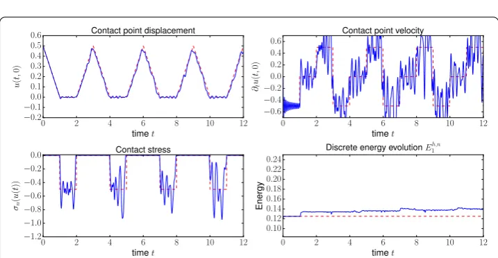
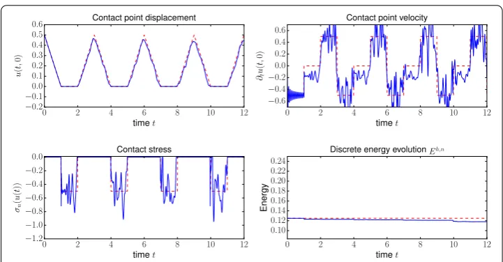
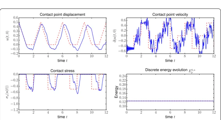
We propose a benchmark associated to multiple impacts. This allows to check both the presence of spurious oscillations and the long term energetic behavior of the method. In the absence of external volume forces, the bar is initially compressed. Then, it is released without initial velocity. It impacts first the rigid ground, located atx= 0, and then gets compressed again. We take the following values for the parameters:f =0,E=1,ρ=1, L=1,u0(x)= 12−x2and ˙u0(x)=0. This problem admits a closed-form solutionuwhich
derivation and expression is detailed in [15]. Notably, it has a periodic motion of period 3. At each period, the bar stays in contact with the rigid ground during one time unit (see Fig.1). The chosen simulation time isT =12, so that we can observe 4 successive impacts.
Numerical results for Nitsche’s method
We discretize the bar withM = 20 linear finite elements (k = 1,h = 0.05) and take
τ =0.01. The resulting Courant number isνC =0.2. Note that almost all the parameters have been taken identical as in [29] for comparison purposes. The number of element is smaller (M=20 instead of 100 in [29]) and the time-stepτis 0.01 for stability reasons. We first investigate the variant=0 with a parameterγ0=1. The mass matrix is computed