Continuum mathematics at the nanoscale

(1)

R E S E A R C H

Open Access

Continuum mathematics at the nanoscale

Tim G Myers

1*

_{, Michelle M MacDevette}

1,2

_{, Francesc Font}

1,2

_{and Vincent Cregan}

1

*_{Correspondence: tmyers@crm.cat} 1_{Centre de Recerca Matemàtica,} Campus de Bellaterra, Ediﬁci C, Bellaterra, Barcelona, 08193, Spain Full list of author information is available at the end of the article

Abstract

In this paper we discuss three examples where continuum theory may be applied to describe nanoscale phenomena:

1. Enhanced ﬂow in carbon nanotubes (CNTs) – This model shows that the experimentally observed enhancement can be explained using standard ﬂow equations but with a depletion layer between the liquid and solid interfaces. 2. Nanoparticle melting – Nanoparticles often exhibit a sharp increase in melting

rate as the size decreases. A mathematical model will be presented which predicts this phenomena.

3. Nanofluids – Experimental results concerning the remarkable heat transfer characteristics of nanofluids are at times contradictory. We develop a model for the thermal conductivity of a nanofluid, which provides much higher predictions than the standard Maxwell model and a better match to data.

Keywords: carbon nanotubes; enhanced ﬂow; nanoparticle melting; thermal conductivity; nanoﬂuid

1 Introduction

Continuum theory may be applied when there is a sufficiently large sample size to en-sure that statistical variation of material quantities, such as density, is small. For fluids the variation is often quoted as % []. Assuming a spherical sample Nguyen and Werely [] suggest this level of variation requires a minimum of _{atoms and so deduce a critical} di-mension of the order  and  nm for liquids and gases respectively. In fact by comparing molecular dynamics (MD) simulations to computations based on the Navier-Stokes equa-tions Travis et al. [] show that continuum theory may be applied to water flow down to around  nm. Thomas et al. [] suggest a figure of . nm. In the field of heat transfer and phase change it has been suggested that continuum theory requires particle radii greater than  nm []. Kofman et al. [] state that at scales smaller than  nm the melting process is discontinuous and dominated by fluctuations, Kuo and Clancy [] observed structural changes and a ‘quasi-molten’ state in their study of nanoparticle melting between - nm. Nanoscale is typically described as involving materials with at least one dimension below  nm [], so there is clearly a range of sizes where continuum theory may be applied to nano phenomena. In this paper we will discuss work carried out in the Industrial Math-ematics Group at the Centre de Recerca Matemàtica using continuum theory to study problems in fluid and heat flow and demonstrate how seemingly anomalous behaviour may be explained without resorting to molecular dynamics or empirically based adjust-ments. Full details of the group’s work in this area may be found in [–]. In Section 

(2)

we will examine the issue of enhanced flow in carbon nanotubes. Many experiments have shown that when water flows through a carbon nanotube the flow rate is orders of magni-tude higher than predicted by classical theory. Early papers [, ] quote factors of around  orders of magnitude, although more recent experiments have shown the true figure is closer to  order []. In our model we employ a concept taken from non-Newtonian fluid dynamics, that of a bi-viscosity fluid, to explain why observed flow rates of water in carbon nanotubes are much higher than that predicted by classical theory. The model also sug-gests a physical interpretation for the Navier slip condition. In Section  we investigate the melting of nanoparticles. As the particles decrease in size, and so the ratio of bulk to sur-face atoms decreases, it becomes easier for sursur-face atoms to leave the particle. This results in a decrease in the melt temperature. Using a form of the Gibbs-Thompson relation to describe the variation of melt temperature with size we produce a model that explains the experimentally observed ‘abrupt melting’. The final problem concerns nanofluids, these are fluids containing a suspension of nanoparticles. They have been claimed to signifi-cantly increase certain fluid properties, such as the thermal conductivity and heat transfer coefficient. Despite hundreds of papers affirming the remarkable heat transfer properties, it was recently shown in a benchmark study, carried out in over thirty laboratories around the world, that nanofluids do not provide significant improvements []. A theoretical demonstration that increasing nanoparticle concentration can decrease heat transfer was shown in []. This contradicted many analytical papers using the same model. However, experiments seem clear that the conductivity of the fluids increases significantly with par-ticle concentration. The classical Maxwell model, to describe the heat conduction of a solid-in-liquid suspension, is known to significantly underpredict the thermal response of a nanofluid. In Section  we investigate the thermal conductivity of a nanofluid. The Maxwell model is based on a static analysis. Using an approximate solution method to the heat flow problem we obtain an expression for the thermal conductivity of the fluid which shows much better agreement with experiment.

A review on the mathematics of the continuum to describe behaviour at the nanoscale can be found in []. Previous mathematical models describing the melting of nanoparti-cles based on continuum theory exist, for instance [–].

2 Enhanced ﬂow in carbon nanotubes

(3)

Fluid flow in a circular pipe is explained by the well-known Hagen-Poiseuille equation which yields the fluid flux expression

QHP= – πR_p

z

μ , ()

whereRis the pipe radius,pzis the pressure gradient along the pipe andμthe ﬂuid

viscos-ity. Research has demonstrated that the ﬂux associated with CNTs is considerably higher than (). To explain this enhancement, a typical approach is to replace the no-slip bound-ary condition,u(R) = , with the slip length formulation

u(R) = –Ls

∂u(R)

∂r , ()

whereLsis the slip length. This leads to a modiﬁed ﬂux expression

Qslip=QHP

 +Ls

R

. ()

Flow enhancement is generally defined as,εslip=Qslip/QHP, the ratio of the observed to predicted fluxes, and thusLshas an obvious effect on any enhancement in the flow. On the

microscale, it has been shown experimentally, that the slip length is much smaller than the channel dimension. In contrast, the slip length for nanochannels is usually of the order of microns. At present, there is no accepted theory for the slip length of a liquid ﬂowing past a solid surface. However, there is one for gases, and the slip length is of the order of the mean free path of the gas []. Holt et al. [] and Majumder et al. [] report slip lengths of the order of microns to match with their corresponding experimental treatments. However, some authors [, ] have questioned the validity of the slip modiﬁed Hagen-Poiseuille model based on the larger slip lengths reported in CNT studies. Cottin-Bizonne et al. [] suggest that the slip length should have a single, radius-independent value and be much smaller than those typically quoted in the literature. In addition, they postulate that the contamination by hydrophobic particles to be the cause of some of the high experimental values. The hydrophobicity of CNTs has been proposed as an alternative explanation to the slip length. Eijkel and van den Berg [] report that the strength of attraction between water molecules is greater than the attractive force between the hydrophobic solid and the water. This hydrophobicity can then lead to some form of ‘depletion layer’ which may be interpreted as a region of low viscosity close to the tube wall. Experimentally this may be viewed in terms of ‘apparent’ slip [, ]. Several authors have observed this phenomenon experimentally [–] and via molecular dynamics simulations [].

We can model the scenario where a fluid flows over a depletion layer by assuming a bi-viscosity flow model. Specifically, the model consists of equations for the bulk flow region in the centre of the channel and a depleted region with low viscosity at the walls of the tube. Matching the velocity and shear stress at the interface of these two regions atr=α results in the flux expression

Qμ=QHP α

R

 +μ μ

R α– 

, ()

(4)

and thusα=R– . nm. The ﬂow enhancement is deﬁned as the ratioεμ=Qμ/QHP. If we take experimental data from Whitby et al. [] we obtainμ≈.μ. Two readily avail-able gases, air and oxygen, have viscosities approximately . that of water.

As highlighted, gas flow theory accounts for apparent slip over a solid surface, but no equivalent theory exists for fluids. By comparing the flux expressions using a slip model and a depletion layer we obtain an expression for the slip length

Ls=δ

μ μ

– 

 –  δ

R+

δ

R

 – 



δ

R



, ()

see []. As predicted by Thomas and McGaughey [] the slip length is a monotonically decreasing function ofR. In addition, noting thatμ/μ, we can identify three distinct tube regimes, namely: wide, moderate and small tubes.

. Forsufficiently wide tubeswhereδ/Rμ/μwe haveεμ≈, and there is no noticeable flow enhancement. As a result the no-slip boundary condition is sufficient. Slip is not observed in wide tubes with smooth surfaces. This condition holds for

R> μm.

. Formoderate tubeswhere(δ/R)(μ/μ)isO()butδ/Rthen only the leading order term ofLsapplies and

εμ≈ + δ

R

μ μ

– 

. ()

This applies approximately forR∈[nm, μm], and reﬂects a constant slip length ofLs=δμ/μ. Several authors [, ] describe constant slip-lengths around

- nm.

. Forvery small tubeswhereδ/RisO()we require the full expression forεμ, and thus the slip length varies withR.

TheRbounds for the diﬀerent regimes are chosen such that there is a maximum error of % when using the approximation.

The present model predictsεμ≈. forR= . nm which is corroborated by Thomas et al. [] who reportεμ≈. The model also predicts a maximum enhancement (obtained by settingR=δ) of approximately  which agrees with the maximum value of  recorded by Whitby et al. [].

3 Nanoparticle melting

(5)

al. [] consider antibiotic and antianginal drugs, which exhibit a melting point depres-sion of around  K. Since gold has low toxicity, gold nanoparticles also make good carri-ers for drug and gene delivery []. Hence, an accurate model to undcarri-erstand the thermal behaviour of a nanoparticle and its probable phase change behaviour is extremely desir-able. In this section we present a mathematical model describing the melting process of nanoparticles proposed by Font and Myers [].

Assuming that density and speciﬁc heat are approximately constant in both the solid and liquid phases, the melt temperature is obtained via the generalised Gibbs-Thomson relation

Lm

Tm

T_m∗ – 

+c

Tmln

Tm

T_m∗

+T_m∗ –Tm

= –σslκ

ρ , ()

whereLmis the latent heat,Tmis the temperature at which the phase change occurs,Tm∗

the bulk phase change temperature,c=cl–csthe change in speciﬁc heat from liquid to

solid,σslthe surface tension andκ the mean curvature. In the present model we assume

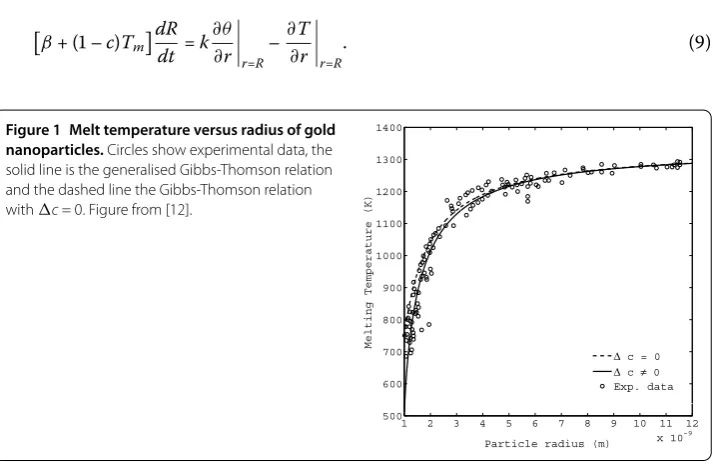
equal density for the solid and liquid phases, which is denoted byρ. For the present analysis we assume that the ambient pressure variation is small, and thus a pressure related term which may appear in this relation is assumed negligible. Figure  compares the generalised Gibbs-Thomson relation against experimental data for gold nanoparticles in the range - nm, see [-].

For the melting of a spherically symmetric particle we consider the dimensionless model

∂T

∂t =



r ∂ ∂r

r∂T

∂r

, ∂θ

∂t = k c



r ∂ ∂r

r∂θ

∂r

, ()

whereTandθdenote the temperature in the liquid and solid, andk,care the solid to liquid conductivity and speciﬁc heat ratios, respectively. The boundary conditions areT(,t) = ,

T(R(t),t) =θ(R(t),t) =Tm, ∂θ∂rr== , wherer=R(t) is the position of the solid-liquid in-terface. The Stefan condition is

β+ ( –c)Tm

dR dt =k

∂θ ∂r

r=R

–∂T ∂r

r=R

. ()

(6)

This model is similar to that described in []: the main diﬀerence being that our Gibbs-Thomson relation includesc. As will be seen later, for large particles this does not greatly aﬀect the results but becomes increasingly important as the particle size decreases.

The dimensionless melting temperatureTmis given by the solution to

 =β

Tm+

R

+( –c) δT

Tm+

 δT

ln(TmδT+ ) –Tm

. ()

The model dimensionless parameters are deﬁned to be

c=cs/cl, k=ks/kl, δT=T/Tm∗, β=

Lm

clT

, = σslT

∗

m

RρLmT

,

whereT=TH–Tm∗ is the temperature change (withTHthe temperature applied at the

nanoparticle surface) andRthe initial particle radius.

For water, gold and lead, for a temperature change ofT=  K we ﬁndβ≈, ,  and smaller increases inTresult in largerβ. As a direct consequence of their small volume, the energy required to melt nanoparticles is also small. In fact any increase above the melting temperature on the nanoparticle surface is enough to almost instantaneously melt it. Thus, we focus exclusively on the large Stefan number regime (i.e.,β). We observe that smallβsuggests a fast melting process as the temperature applied at the nanoparticle surface,TH, is much greater than the melting temperature,Tm∗. On the other hand largeβ

indicates a slower process asTHis closer toTm∗. (However, we note that the time-scales are

of the order of pico seconds, so slow and fast are relative terms.) This implies a relationship between β and the time-scale. Hence we rescale viat=βτ and search for asymptotic solutions of the formT=T+T/β+O(/β). In the case of the liquid we have the systems

O():  = 

r ∂ ∂r

r∂T

∂r

, T(,τ) = , T(R,τ) =Tm, ()

O(/β): ∂T ∂τ =  r ∂ ∂r

r∂T

∂r

, T(,τ) = , T(R,τ) = , ()

with corresponding solutions

T=  + (Tm– )

R r

 –r

 –R

, ()

T=μ ( –r)r–  r –R r  –r

 –R

( –R)R–

R

dR

dτ, ()

where

μ=  ( –R)

β

R[β+(–_δ_Tc)ln(TmδT+ )]

+(Tm– ) ( –R)

. ()

In the solid

θ=Tm, θ= –μ

R–rdR

(7)

where

μ=

c

k

β

R_[β₊(–c)

δT ln(TmδT+ )]

. ()

The Stefan condition is

dR dτ =

(Tm– )

R( –R)

 +  β

( –c)Tm– μ ( –R)

R – kμR

–

, ()

and this is coupled to the diﬀerentiated version of the Gibbs-Thomson equation

dTm

dτ =

R_[+(–c)

βδTln(TmδT+ )]

dR

dτ. ()

The initial conditions for the above coupled system of equations isR() =  andTm() =

Tm(), where the latter value is ﬁxed by solving () withR= . Hence, the problem has

been reduced considerably from a system of two heat equations in the solid and liquid de-fined over a changing domain specified by the Stefan condition and coupled to an equation describing the phase change temperature to solving two first order ODEs.

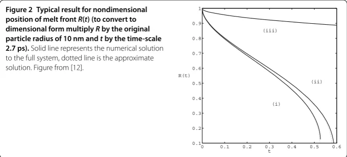
Figure  illustrates the evolution of the melt front,R(t), where the dotted and solid lines are the approximate solution and a numerical solution to the full system, respectively. The three sets of curves denote three associated sets of solutions. Speciﬁcally, the curves la-belled (i) denote the model using the generalised Gibbs-Thomson relation, curves (ii) take

cs=clin Gibbs-Thomson but not the energy balance (see []) and curves (iii) are the

stan-dard model whereTm=Tm∗ andcs=cl. Clearly, the standard model overestimates the melt

time considerably. Curves (i) and (ii) show that as the solid radius decreases, the gradient of the curve increases rapidly and tends to infinity. Physically, this implies that in the final stages of melting, the particle will suddenly vanish, and this is the ‘abrupt melting’ phe-nomena reported by []. Figure  presents the temperature profile within the liquid and solid regions as the particle melts. The circles show how the melt temperature decreases with time, the dotted line is the solid phase temperature and the solid line is the liquid temperature. An interesting feature of this graph is the fact that the solid temperature is greater than the phase change temperature. In a standard problem the solid would be

(8)

Figure 3 Temperature proﬁles within a melting nanoparticle.Figure from [12].

low the phase change temperature and so slow down the process, in this case the decrease in melt temperature means the solid actually acts to speed up the melting.

4 Thermal conductivity of nanoﬂuids

The enhanced thermal properties of nanofluids, compared to their base fluids, has led nanofluids to being an attractive solution for heat removal in modern electronic devices [, ]. Consequently, the study of the thermal properties of nanofluids is an intense research area. One of the critical ongoing issues is the lack of a satisfactory theoretical model for the thermal response of a nanofluid [, ].

Based on eﬀective medium theory, Maxwell’s seminal theoretical description of heat conduction in solid-in-liquid suspensions [] yields the eﬀective thermal conductivity

ke

kl

=

kl+kp+ φ(kp–kl)

kl+kp–φ(kp–kl)

, ()

whereke,kp,kldenote the eﬀective, particle and liquid thermal conductivity andφis the

particle volume fraction. The Maxwell model has several well-known drawbacks. Fore-most, the model is only applicable to heat flow in the material surrounding an equivalent fluid or around a particle, and not the scenario of interest, namely, an actual nanofluid or particle. Secondly, the theory is based on an infinite region [] and hence is only applica-ble to very dilute solutions where the particles are sufficiently far apart such that there is negligible thermal interaction between the particles. Clearly, this will lead to problems if the particle concentration increases. In addition, Maxwell’s theory is based on a steady-state analysis, which restricts one from considering the more interesting time dependent thermal response of the nanofluid.

Despite the aforementioned limitations, the Maxwell model works well for low volume fraction ﬂuids with relatively large particles. However, the accuracy of the model deteri-orates when the particle size decreases to the nanoscale. Keblinski et al. [] compared experimental data from various nanoﬂuid treatments and reported that in most cases

ke≈( +Ckφ)klwithCk≈, which is in contrast to the linearised Maxwell model where

Ck≈. To improve the ﬁt between data and theory, numerous authors have proposed

(9)

example, Prasher et al. [] and Koo and Kleinstreuer [] modify Maxwell’s result to ac-count for Brownian motion. Yu and Choi [] introduce a nanolayer of width  nm with a thermal conductivity ten times greater than that of the base fluid. The extensive review of Das et al. [] illustrates that with the inclusion of additional effects and new parameters, there is better agreement between experiment and the variants of Maxwell’s theory. In this section we discuss an alternative expression for the thermal conductivity of a nanofluid re-cently proposed by Myers et al. [] that agrees well with experimental data.

If we focus on the liquid diﬀusion time-scale, then a suitable dimensionless model for heat ﬂow through a spherically symmetric liquid-particle system is given by

∂T

∂t =

α

r ∂ ∂r

r∂T

∂r

, r∈[,rp], ()

∂θ ∂t =



r ∂ ∂r

r∂θ

∂r

, r∈[rp, ], ()

where T andθ are the temperatures in the particle and ﬂuid, respectively,α=αp/αl is

the ratio of the particle and liquid thermal diﬀusivities andrp is the particle radius. We

impose a fixed boundary temperature greater than the initial temperature and continuity of temperature and heat flux at the fluid-particle interface. Thus, the relevant conditions are

θ(r, ) =T(r, ) = , θ(,t) = , θ(rp,t) =T(rp,t) =Tp(t),

∂θ ∂r

r=rp

=k∂T

∂r

r=rp

, ∂T

∂r

r=

= , ()

wherek=kp/kl.

To ascertain the effective thermal conductivityke, we first examine an ‘equivalent fluid’

with diﬀusivityαe. Hence, we consider the system

∂θe

∂t =

αe

r ∂ ∂r

r∂θe

∂r

, θe(,t) = ,

∂θe

∂r

r=

= , ()

which is easily solved to give a solution in terms of Bessel’s functions. Of particular interest is the temperature at the centre given by

θe(,t) =θs(t) =  + N

n=

(–)ne–nπαet_. _()

The associated particle-fluid system is more complex and requires approximate solution methods. Firstly, we note that to increase the base fluid thermal conductivity, we introduce nanoparticles with a much higher diffusivity relative to the base fluid. For example, copper and AlO in water or ethylene-glycol solutions, have α andk. In effect, this indicates that heat is transferred more rapidly through the particle than the fluid, and henceT(r,t)≈Tp(t). The fluid thermal problem is reduced to a Cartesian system via the

(10)

expressions, and thus highlight the inﬂuence of the physical parameters in the model. The solution to the HBIM yields

Tp=  –e–(t–t), ()

wheretis the time when the particle temperature ﬁrst rises noticeably above the initial temperature,=nλ/cT,λ= /( –rp) andcT= ( +rp)/ – /(n+ ). From [, ] the

constantn= . is found by minimising the least-squares error when the approximate solution is substituted into the heat equation.

Similarly, we apply the HBIM to the equivalent ﬂuid system to obtain the centre tem-perature

Tc=  –e–

₍_t_–_t

)_, _()

where=nαe/cTandcT= (n– )/((n+ )). The accuracy of this formula may be veri-ﬁed by comparison with the exact solution ().

As the HBIM solution is an acceptable approximation, we find an comparable diffusivity by a matching argument between the HBIM solution for a particle and that of an equiva-lent fluid. Hence, we adopt a simple approach and equate the decay rates in the expressions forTpandTc. This is equivalent to setting=which yields

αe=

αl

( –rp)

n–  (n+ )

 +rp

 –



n+  –

. ()

The dimensionless radiusrpis scaled with the ﬂuid radiusR. Typically, these relations are

posed in terms of the volume fractionφwhererp=φ/, and thus

αe=

αl

( –φ/₎

n–  (n+ )

 +φ/

 –



n+  –

. ()

A cursory glance of the above expression reveals that the thermal diffusivity of the equiv-alent fluid depends only on the liquid diffusivity and volume fraction. Critically, the com-position of the nanoparticle does not affectαe. Via [], using the relationsαe=ke/(ρc)e

and (ρc)e=φρpcp+ ( –φ)ρlcl, we may write the eﬀective thermal conductivity as

ke

kl

= [( –

φ) +φρ_ρpcp

lcl](n– )

( –φ/₎_{[( +}_φ/₎₍_n_{+ ) – ]}, ()

which indicates that the equivalent particle conductivity is independent of the particle conductivity. Note this has been veriﬁed experimentally, see [, ]. The particle material properties appear through the density and heat, (ρc)p. However, as the ratioρpcp/(ρlcl) is

O() andφis small, this is a weak dependence. Consequently, the eﬀective conductivity is predominantly a function of the liquid conductivitykland volume fractionφ.

(11)

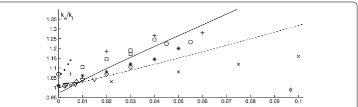
Figure 4 Conductivity ratioke/klfor Al2O3-water nanoﬂuid withkl= 0.58 W/mK.Equation()(solid

line); Maxwell model equation()(dashed line) and experimental data. Figure from [13].

theory and models the data better. However, forφ> ., the present model rapidly in-creases above the Maxwell theory, and more signiﬁcantly, passes through a larger amount of the data. Thus the present model clearly out performs the basic Maxwell model for the majority of the experimental data for volume fractions greater than %.

5 Conclusion

This paper provides a brief overview of three pertinent problems from the nano field. In the first problem we considered a model for fluid flow in carbon nanotubes. At present there is no theory for calculating the slip lengths for a liquid moving over a solid surface. We used an equivalent theory with a depletion layer over a solid surface to obtain an ex-pression for the slip length in terms of the depletion layer thickness and its viscosity. Next, we presented a mathematical model that successfully captured the ‘abrupt melting’ phe-nomenon of nanoparticles. In particular, the model demonstrated the sharp increase in melting rate as the size of the nanoparticles decreased. Finally, we considered the ther-mal conductivity of nanofluids, and our analysis led to an expression for solid-in-liquid suspensions, derived in a distinct way to the seminal Maxwell model. The model showed excellent agreement with experimental data for particle volume fractions greater than %. While this work is at the limit of continuum theory, in each case the continuum mod-els demonstrated good agreement with experimental data and provided valuable insight. Moreover, the results of the nanoscale modelling in some cases led to a deeper under-standing of the macroscale problems. At present there is great interest in nanotechnology with applications in a wide range of areas. We have presented results for just three spe-cific problems, however the success of the models indicates that there is great scope for applying continuum models at the nanoscale.

Competing interests

The authors declare that they have no competing interests.

Authors’ contributions

All authors contributed equally to the writing of this paper. All authors read and approved the ﬁnal manuscript.

Author details

1_{Centre de Recerca Matemàtica, Campus de Bellaterra, Ediﬁci C, Bellaterra, Barcelona, 08193, Spain.}2_{Departament de} Matemàtica Aplicada I, Universitat Politècnica de Catalunya, Barcelona, Spain.

Acknowledgements

(12)

Received: 19 December 2013 Accepted: 18 August 2014 Published:08 Sep 2014 References

1. Abragall P, Nguyen N-T:Nanoﬂuidics. 1st edition. Norwood: Artech House; 2009.

2. Nguyen N-T, Werely ST:Fundamentals and Applications of Microﬂuidics. 2nd edition. Norwood: Artech House; 2006. 3. Travis KP, Todd BD, Evans DJ:Departure from Navier-Stokes hydrodynamics in conﬁned liquids.Phys Rev E1997,

55(4):4288-4295.

4. Thomas JA, McGaughey AJH, Ottoleo K-A:Pressure-driven water ﬂow through carbon nanotubes: insights from molecular dynamics simulation.Int J Therm Sci2010,49(2):281-289.

5. Guisbiers G, Kazan M, Van Overschelde O, Wautelet M, Pereira S:Mechanical and thermal properties of metallic and semiconductive nanostructures.J Phys Chem C2008,112:4097-4103.

6. Kofman R, Cheyssac P, Lereah Y, Stella A:Melting of clusters approaching 0D.Eur Phys J D1999,9(1-4):441-444. 7. Kuo C-L, Clancy P:Melting and freezing characteristics and structural properties of supported and unsupported

gold nanoclusters.J Phys Chem B2005,109:13743-13754.

8. Das SK, Choi SU, Yu W, Pradeep T:Nanoﬂuids: Science and Technology. 1st edition. New York: Wiley; 2008. 9. Myers TG:Optimizing the exponent in the heat balance and reﬁned integral methods.Int Commun Heat Mass

Transf2009,36(2):143-147.

10. Myers TG:Optimal exponent heat balance and reﬁned integral methods applied to Stefan problems.Int J Heat Mass Transf2010,53(5-6):1119-1127.

11. Myers TG:Why are slip lengths so large in carbon nanotubes?Microﬂuid Nanoﬂuid2011,10(5):1141-1145 [doi:10.1007/s10404-010-0752-7].

12. Font F, Myers TG:Spherically symmetric nanoparticle melting with a variable phase change temperature. J Nanopart Res2013,15(12):2086 [doi:10.1007/s11051-013-2086-3].

13. Myers TG, MacDevette MM, Ribera H:A time-dependent model to determine the thermal conductivity of a nanoﬂuid.J Nanopart Res2013,15(7):1775 [doi:10.1007/s11051-013-1775-2].

14. Font F, Myers TG, Mitchell SL:A mathematical model for nanoparticle melting with density change.Microﬂuid Nanoﬂuid2014 [doi:10.1007/s10404-014-1423-x].

15. Holt JK, Park HG, Wang Y, Stadermann M, Artyukhin AB, Grigoropoulos CP, Noy A, Bakajin O:Fast mass transport through sub-2-nanometer carbon nanotubes.Science2006,312(5776):1034-1037.

16. Majumder M, Chopra N, Andrews R, Hinds BJ:Nanoscale hydrodinamics: enhanced ﬂow in carbon nanotubes. Nature2005,438:44.

17. Whitby M, Cagnon L, Thanou M, Quirke N:Enhanced ﬂuid ﬂow through nanoscale carbon pipes.Nano Lett2008,

8(9):2632-2637.

18. Buongiorno J, Venerus DC, Prabhat N, McKrell T, Townsend J, Christianson R, Tolmachev YV, Keblinski P, Hu L-w, Alvarado JL, Bang IC, Bishnoi SW, Bonetti M, Botz F, Cecere A, Chang Y, Chen G, Chen H, Chung SJ, Chyu MK, Das SK, Di Paola R, Ding Y, Dubois F, Dzido G, Eapen J, Escher W, Funfschilling D, Galand Q, Gao J, Gharagozloo PE, Goodson KE, Gutierrez JG, Hong H, Horton M, Hwang KS, Iorio CS, Jang SP, Jarzebski AB, Jiang Y, Jin L, Kabelac S, Kamath A, Kedzierski MA, Kieng LG, Kim C, Kim J-H, Kim S, Lee SH, Leong KC, Manna I, Michel B, Ni R, Patel HE, Philip J, Poulikakos D, Reynaud C, Savino R, Singh PK, Song P, Sundararajan T, Timofeeva E, Tritcak T, Turanov AN, Van Vaerenbergh S, Wen D, Witharana S, Yang C, Yeh W-H, Zhao X-Z, Zhou S-Q:A benchmark study on the thermal conductivity of nanoﬂuids.J Appl Phys2009,106(9):094312.

19. MacDevette MM, Myers TG, Wetton B:Boundary layer analysis and heat transfer of a nanofluid.Microfluid Nanofluid 2014,17(2):401-412 [doi:10.1007/s10404-013-1319-1].

20. Thamwattana N, Hill JM, Baowan D, Cox BJ:A review of mathematical and mechanical modelling in nanotechnology.Math Mech Solids2010,15:708-717.

21. Wu T, Liaw H-C, Chen Y-Z:Thermal effect of surface tension on the inward solidiﬁcation of spheres.Int J Heat Mass Transf2002,45(10):2055-2065.

22. Wu B, McCue SW, Tillman P, Hill JM:Single phase limit for melting nanoparticles.Appl Math Model2009,

33(5):2349-2367.

23. McCue SW, Wu B, Hill JM:Micro/nanoparticle melting with spherical symmetry and surface tension.IMA J Appl Math2009,74:439-457.

24. Meyyappan M:Carbon Nanotubes: Science and Applications. 1st edition. Boca Raton: CRC Press; 2004.

25. Pantarotto D, Singh R, McCarthy D, Erhardt M, Briand J-P, Prato M, Kostarelos K, Bianco A:Functionalized carbon nanotubes for plasmid DNA gene delivery.Angew Chem, Int Ed Engl2004,43(39):5242-5246

[doi:10.1002/anie.200460437].

26. Wang J:Carbon-nanotube based electrochemical biosensors: a review.Electroanalysis2005,17(1):7-14. 27. Zanello LP, Zhao B, Hu H, Haddon RC:Bone cell proliferation on carbon nanotubes.Nano Lett2006,6(3):562-567. 28. Suzuki K, Yamaguchi M, Kumagai M, Yanagida S:Application of carbon nanotubes to counter electrodes of

dye-sensitized solar cells.Chem Lett2003,32(1):28-29 [doi:10.1246/cl.2003.28].

29. Heinze S, Tersoﬀ J, Martel R, Derycke V, Appenzeller J, Avouris P:Carbon nanotubes as Schottky barrier transistors. Phys Rev Lett2002,89:106801 [doi:10.1103/PhysRevLett.89.106801].

30. White FM:Viscous Fluid Flow. 1st edition. New York: McGraw-Hill; 1991.

31. Thomas JA, McGaughey AJH:Reassessing fast water transport through carbon nanotubes.Nano Lett2008,

8(9):2788-2793.

32. Verweij H, Schillo MC, Li J:Fast mass transport through carbon nanotube membranes.Small2007,3(12):1996-2004. 33. Cottin-Bizonne C, Cross B, Steinberger A, Charlaix E:Boundary slip on smooth hydrophobic surfaces: intrinsic

effects and possible artifacts.Phys Rev Lett2005,94:056102.

34. Eijkel JT, van den Berg A:Nanofluidics: what is it and what can we expect from it?Microfluid Nanofluid2005,

1(3):249-267.

35. Neto C, Evans DR, Bonaccurso E, Butt H-J, Craig VSJ:Boundary slip in Newtonian liquids: a review of experimental studies.Rep Prog Phys2005,68(12):2859 [http://stacks.iop.org/0034-4885/68/i=12/a=R05].

(13)

37. Joseph S, Aluru NR:Why are carbon nanotubes fast transporters of water?Nano Lett2008,8(2):452-458. 38. Barrat J-L, Bocquet L:Inﬂuence of wetting properties on hydrodynamic boundary conditions at a ﬂuid/solid

interface.Faraday Discuss1999,112:119-128.

39. Matthews MT, Hill JM:Nanoﬂuidics and the Navier boundary condition.Int J Nanotechnol2008,5(2/3):218-242. 40. Choi C-H, Westin KJA, Breuer KS:Apparent slip ﬂows in hydrophilic and hydrophobic microchannels.Phys Fluids

2003,15(10):2897-2902.

41. Shim J-H, Lee B-J, Cho YW:Thermal stability of unsupported gold nanoparticle: a molecular dynamics study.Surf Sci2002,512:262-268.

42. Buﬀat P, Borel JP:Size effect on the melting temperature of gold particles.Phys Rev A1976,13(6):2287-2297. 43. Bergese P, Colombo I, Gervasoni D, Depero LE:Melting of nanostructured drugs embedded into a polymeric

matrix.J Phys Chem B2004,108:15488-15493.

44. Liu X, Yangb P, Jiang Q:Size effect on melting temperature of nanostructured drugs.Mater Chem Phys2007,

103:1-4.

45. Rana S, Bajaj A, Mout R, Rotello VM:Monolayer coated gold nanoparticles for delivery applications.Adv Drug Deliv Rev2012,64:200-216.

46. Nguyen CT, Roy G, Gauthier C, Galanis N:Heat transfer enhancement using Al2O3-water nanoﬂuid for an electronic liquid cooling system.Appl Therm Eng2007,27(8-9):1501-1506

[doi:10.1016/j.applthermaleng.2006.09.028].

47. Yu W, France DM, Routbort JL, Choi SUS:Review and comparison of nanoﬂuid thermal conductivity and heat transfer enhancements.Heat Transf Eng2008,29(5):432-460.

48. Prasher R, Bhattacharya P, Phelan PE:Thermal conductivity of nanoscale colloidal solutions (nanoﬂuids).Phys Rev Lett2005,94:025901.

49. Maxwell JC:A Treatise on Electricity and Magnetism. Volume 1. 3rd edition. Oxford: Clarendon Press; 1881. 50. Keblinski P, Eastman JA, Cahill DG:Nanoﬂuids for thermal transport.Mater Today2005,8(6):36-44. 51. Koo J, Kleinstreuer C:A new thermal conductivity model for nanoﬂuids.J Nanopart Res2004,6(6):577-588

[doi:10.1007/s11051-004-3170-5].

52. Yu W, Choi SUS:The role of interfacial layers in the enhanced thermal conductivity of nanoﬂuids: a renovated Maxwell model.J Nanopart Res2003,5(1-2):167-171 [doi:10.1023/A:1024438603801].

53. Zhou S-Q, Ni R:Measurement of the speciﬁc heat capacity of water-based Al2O3nanoﬂuid.Appl Phys Lett2008,

92(9):093123.

10.1186/2190-5983-4-11

Cite this article as:Myers et al.:Continuum mathematics at the nanoscale.Journal of Mathematics in Industry