http://www.sciencepublishinggroup.com/j/ajtas doi: 10.11648/j.ajtas.20170606.17
ISSN: 2326-8999 (Print); ISSN: 2326-9006 (Online)
Construction of Weighted Second Order Rotatable Simplex
Designs (Wrsd)
Otieno-Roche Emily
1, Koske Joseph
2, Mutiso John
21Department of Computer and Information Technology, Africa Nazarene University, Nairobi, Kenya 2
Department of Statistics and Computer Science, Moi University, Eldoret, Kenya
Email address:
[email protected] (Otieno-Roche E.), [email protected] (Koske J.), [email protected] (Mutiso J.)
To cite this article:
Otieno-Roche Emily, Koske Joseph, Mutiso John. Construction of Weighted Second Order Rotatable Simplex Designs (Wrsd). American Journal of Theoretical and Applied Statistics. Vol. 6, No. 6, 2017, pp. 303-310. doi: 10.11648/j.ajtas.20170606.17
Received: June 2, 2017; Accepted: June 16, 2017; Published: December 7, 2017
Abstract:
Response surface methodology is widely used for developing, improving, and optimizing processes in various fields. A rotatable simplex design is one of the new designs that have been suggested for fitting second-order response surface models. In this article, we present a method for constructing weighted second order rotatable simplex designs (WRSD) which are more efficient than the ordinary rotatable simplex designs (RSD). Using moment matrices based on the Simplex and Factorial Designs, and the General Equivalence Theorem (GET) for D- and A- optimality, weighted rotatable simplex designs (WRSDs) were obtained. A- and D- optimality criterion was then used to establish the efficiency of the designs.Keywords:
D – Optimal, A – Optimal, Response Surface Designs, Second-Order Designs, Information Surface, Moment Matrices, Weighted Rotatable Simplex Designs1. Introduction
A rotatable simplex design is one of the newly introduced designs in response surface experiment. Rotatable Simplex Designs have been suggested to have a very wide usage e.g in Food science, Business performance, Health sciences, Bio-processing, Engineering, Construction Industry and so on as its performance was illustrated in Response Surface Analysis (RSA) of percentage crude oil removed by three factors. Rotatable Simplex Designs (RSDs) are constructed using the properties of a Simplex – lattice design (SLD), through Full Factorial Designs (FFDs)
Design points from SLD are used to generate the original design points for the RSD. The levels of the SLD were increased by taking all the combination levels of the original points from the SLD such that the sum of all odd moments is zero. These points were then augmented with all the combination levels of the distance from the centre point ( ). Equation (1) was then solved to attain rotatability.
∑ = 3 ∑ ≠ (1)
where the summation in the above relations is over the design points = 1, 2, … , .
The introduction of weights to RSD in this paper is for the purpose of improving the design by making it more efficient
2. Optimality Criteria and Efficiencies
Optimal designs are experimental designs that are generated based on a particular optimality criterion and are generally optimal only for a specific statistical model. The ultimate purpose of any optimality criterion is to measure the largeness of a non-negative definite × information matrix
C.
The optimality criterion used in this study were from the family of matrix means ∅ = −1, 0, introduced by Kiefer (1964) and is discussed in detail by Pukelsheim (1993).
Efficiency tests the goodness of a design.
3. Weighted Rotatable Simplex Designs
A WRSD is modified from the general RSD by separating it into Simplex and “Radius” Factorial blocks having weights
! and assigned to the Simplex block "#!$ and ‘Radius’ factorial block "# $.
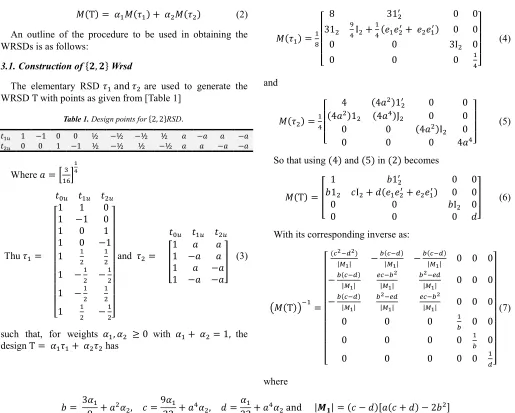
&"Τ$ = !&"#!$ + &"# $ (2) An outline of the procedure to be used in obtaining the WRSDs is as follows:
3.1. Construction of )*, *+ Wrsd
The elementary RSD #! and # are used to generate the WRSD Τ with points as given from [Table 1]
Table 1. Design points for )2, 2+RSD.
! 1 −1 0 0 ½ −½ −½ ½ − −
0 0 1 −1 ½ −½ ½ −½ − −
Where = 0!213 4 5
Thu #!=
6 ! 7 8 8 8 8 8 8 8 8
91 11 −1 0 0 1 0 1 1 0 −1
1 ! !
1 −! −! 1 −! ! 1 ! −!:;
; ; ; ; ; ; ; <
and # =
6 !
= 1 1 −
1 −
1 − −
> (3)
such that, for weights !, ≥ 0 with !+ = 1, the design Τ = !#!+ # has
&"#!$ =!@
7 8 8 8
9 8 31B 0 0
31 CI +!"E!EB+ E E!B$ 0 0
0 0 3I 0
0 0 0 !:;
; ; <
(4)
and
&"# $ =! 7 8 8
9 4"4 $1 "4 $1"4 $JB 00 00 0 0 "4 $I 0
0 0 0 4 :;
; <
(5)
So that using "4$ and "5$ in "2$ becomes
&"Τ$ = =
1 I1B 0 0
I1 JI + K"E!EB+ E E!B$ 0 0
0 0 II 0
0 0 0 K
> (6)
With its corresponding inverse as:
L&"Τ$MN!=
7 8 8 8 8 8 8 8 8 8
9"OP|SNQ4|P$ −
T"ONQ$ |S4| −
T"ONQ$
|S4| 0 0 0 −T"ONQ$|S4| UONT|S4|P T|SPNUQ4| 0 0 0 −T"ONQ$|S4| T|SPNUQ4| UONT|S4|P 0 0 0
0 0 0 T! 0 0
0 0 0 0 !T 0
0 0 0 0 0 !Q:;
; ; ; ; ; ; ; ; < (7) where
I = 3 8 + , J =! 9 32 + , K =! 32 + and |W! X| = "J − K$Y "J + K$ − 2I Z
3.2. )*, *+ Optimal Designs
Optimal designs are experimental designs that are generated based on a particular optimality criterion and are generally optimal only for a specific statistical model. Here we have used the general equivalence theorem to compute the values of the masses assigned to the design points of the RSD to obtain D-optimal and A-optimal WRSDs. Optimality measures the largeness of a non-negative definite × matrix [ where C is the subset of M. In this study, the matrix [ will be the information matrix based on the full parameter system of the model.
3.2.1. D – Optimal Wrsd
A weighted design \" $ is D-optimal for ]B"^$ if and only if
traceLCdC"α$N!M f= JE "[" $
6$ ∈ )1, 2+
< JE "[" $6$ ℎE j E (8)
D – optimal WRSD design therefore is:
ΤL "k$M =
!#!+ # (9)
Where the GET in "7$ is used to obtain the values of ! and which would give a D-optimal design. i.e ! and are solved to satisfy
JE m&"# $ L&"Τ$MN!n = JE"&"Τ$$6, for = 1, 2 (10)
7 8 8 8 8 8
9 "ONQ$"N "OqQ$q1T$|S4| m
"ONQ$"N1q@T$ @|S4| n 1
B 0 0
m"ONQ$YN2"OqQ$qrTZ!2|S4| n 1 mN T|SPqOqQ4| n I + m−N@TPNOq! T"ONQ$qCQ1 |S4| n J 0 0
0 0 m@T1n I 0
0 0 0 1 Q! :;
; ; ; ; <
(11)
With its trace being
! @08 m
"OPNQP$
|WX| n + 12 m−
T"ONQ$ |WX| n +
CmUONTP |WX|n +
!mTPNUQ |WX| n +
2 T+
!
Q3 (12)
and
JE"&"Τ$$6 = JE s
2= 6 (13)
now using (12) and (13) in (9), with !+ = 1, we obtain
!r− 11.6781 !− 40.7289 !1− 46.8974 !+ 16.84662 != 0 (14)
This gives != 0.283748894 for !∈ Y0, 1Z and = 1 − 0.283748894 = 0.716251105
Thus using (3) in (9) together with values of ! and from (14), the unique D – optimal moment matrix for )2, 2+ WRSD is
u
1 0.41661B 0 0
0.41661 0.2141I + 0.1432"E!EB+ E E!B$ 0 0
0 0 0.4166I 0
0 0 0 0.1432
v (15)
3.2.2. A – Optimal Wrsd
A convex combination
\" $ = ∑ \ ,w
x! (16)
with
= " !, , … … … , w$B∈ Τ (17)
is a weighted design with weight vector where
∑ = 1w
x! (18)
From the Kiefer-Wolfowitz equivalence theorem in Pukelsheim (1993), if \" $ satisfies the side condition [ym&L\" $Mn ∈ z{" $ and [ written as [ = [yL&"\ $M
for = 1, … … , |, then, \" $ Solves the design problem i.e the ^~ optimal design problem if for • = −1
Trace [ [yL&"\" $M$N = trace [y"&"\" $$$N! = 1, … … , | (19)
Therefore, a WRSD \" $ is A-optimal if and only if (19) is satisfied
From (6), let "&"Τ$$N!= m€N! 0
0 •N!n so that
"&"Τ$$N = m€N 0
0 •N n (20)
Where € = ‚ 1 I1
B
I1 JI + K"E!EB+ E E!B$ƒ and • =
mII0 Kn0 This gives
€N!= ‚ E 1B
1 „I + ℎ"E!EB+ E E!B$ƒ and • N! = …
!
TI 0
0 !Q† (21)
Similarly, "€N!$ = ‚ 2 + E "ℎ + „ + E$1
B
"ℎ + „ + E$1 "ℎ + „ + $I + "2„ℎ + $"E!EB+ E E!B$ƒ
and
"•N! $ = … !
TPI 0
0 Q!P
† (22)
‡ ˆ ‰
Š1B 0 0
Š1 I + "E!EB+ E E!B$ 0 0
0 0 T!PI 0
0 0 0 Q!P‹
Œ •
(23)
Where
= 2 + E , Š = "ℎ + „ + E$, = ℎ + „ + and = 2„ℎ + In which;
E =J − K|Ž| , =−I"J − K$|Ž| , „ = J − I|Ž| and ℎ =I − K|Ž|
Thus &"#!$"&"Τ$N $ becomes
! @
‡ ˆ ˆ ‰
8 + 6Š "8Š + 3 + 3 $1B 0 0
m3 +!6Šn 1 m3Š +C +! n I + m3Š +C +! n "E!EB+ E E!B$ 0 0
0 0 T1PI 0
0 0 0 !QP‹
Œ Œ •
(24)
and
JEL&"#!$"&"Τ$N $M =!@m8 + 12Š +C +! +T2P+ Q!Pn (25)
with
= •4P
"2 |•|$PY"6 !+ 6.9282 $ + "5 !+ 6 $ Z Š = •4P
"2 |•|$PY"6 !+ 6.9282 $ Y"7 !+ 6.7846 $ + "9 !+ 9.2154 $ + "5 !+ 6 $ ZZ = •4P
"2 |•|$PY "7 !+ 6.7846 $ + "9 !+ 9.2154 $ + "6 !+ 6.9282 $ Z = •4P
"2 |•|$PY"9 !+ 9.2154 $"7 !+ 6.7846 $ + "6 !+ 6.9282 $ Z |€| =! !0 •4
Pq . 16@•4•P
2 3
Now from [20],
JE"&"Τ$N!$ = E + 2„ + T+
!
Q (26)
Using (25) and (26) in (19) results in
1 + 11.0408 !+ 18.1390 !− 55.7918 !1− 214.6311 ! − 1189.2271 !r− 2567.6833 !2+ 2528.7509 !‘−
1273.3248 !@− 254.5424 !C= 0 (27)
Which when solved within Y0, 1Z we get != 0.279637843 and = 1 − != 0.720362156
Hence the unique A-optimal design is
η"α“$ = 0.279637843τ
!+ 0.720362156τ (28)
using (4$ and "5$ together with ! and values from "27$ in (9), we have
u
1 0.41681B 0 0
0.41681 0.2137I + 0.1438"E!EB+ E E!B$ 0 0
0 0 0.4168I 0
0 0 0 0.1438
v (29)
3.3. •–—˜™š›œ™•–— –ž )Ÿ, *+ Wrsd
Similar to 3.1 above, the elementary RSD #! and # are used to generate the WRSD Τ such that: For weights !, ≥ 0 with !+ = 1, the design Τ = !#!+ #
Has the moment matrix "2$ i.e. &"Τ$ = !&"#!$ + &"# $ Where
#!=
6 ! 1
7 8 8 8 8 8 8 8 8 8 8 8 8 8 8 8 8 8 8 8 8 8 8 8 8
911 −1 1 0 0 00 1 0 1 0 1 0 −1 0 1 0 0 1
1 0 0 −1
1 ! ! 0
1 −! ! 0 1 ! −! 0 1 −! −! 0
1 ! 0 !
1 −! 0 ! 1 ! 0 −! 1 −! 0 −!
1 0 ! !
1 0 −! ! 1 0 ! −! 1 0 −! −!:;
; ; ; ; ; ; ; ; ; ; ; ; ; ; ; ; ; ; ; ; ; ; ; <
and # =
6 ! 1
7 8 8 8 8 8 8
91 −1 − − − −
1 − −
1 −
1 − −
1 −
1 −
1 :;
; ; ; ; ; < (30)
From (30) we have:
&"#!$ =!@!
‡ ˆ ‰
18 411B 0 0
411 CI1+!J1 0 0
0 0 4I1 0
0 0 0 !I1‹
Œ •
(31)
and
&"# $ =!@
‡ ˆ
‰ 8 "8 $11
B 0 0
"8 $11 "8 $J1 0 0
0 0 "8 $I1 0
0 0 0 "8 $I1‹
Œ •
(32)
So that (2) becomes
‡ ˆ ˆ ˆ
‰ 1 m
•4
C + n 11B 0 0
m •4
C + n 11 ! @I1+ m
•4
‘ + n J1 0 0
0 0 m •4
C + n I1 0
0 0 0 m•4
‘ + n I1‹
Œ Œ Œ •
(33)
3.4. )Ÿ, *+ Optimal Designs
Similarly, the general equivalence theorem is used to compute the values of the masses assigned to the design points of the RSD to obtain D-optimal and A-optimal WRSDs
3.4.1. D – Optimal Wrsd
D – optimal WRSD design is:
\L "k$M = !#!+ #
such that:
&"Τ$ = !&"#!$ + &"# $ (34) Using the GET to obtain values of ! and which would give a D-optimal design. i.e solving ! and to satisfy
JE m&"# $ L&"Τ$MN!n = JE"&"Τ$$6 = 1, 2 (35)
&"#!$ L&"Τ$MN! is as in APENDIX I
∴ JE m&"#!$ L&"Τ$MN!n
=!@! 0!@"ONQ$P"Oq Q$N! T"ONQ$|•| P+|•|1 0r"ONQ$¡¢"OqQ$N TP£+LTPN¢QM"ONQ$− 4I"J − K$ 3 +!T + 1Q3 (36)
and
JE"&"Τ$$6 = JE I
!6= 10 (37)
now using (36) and (37) in (34) with !+ = 1, we obtain
1 − 3.564144 !+ 5.924622 !− 5.2839 !1+ 3.4871 !− 4.36076 !r+ 0.5915 !2= 0 (38)
This gives != 0.596127182 for !∈ Y0, 1Z, and = 1 − 0.596127182 = 0.403872817
Therefore using (30) with ! and values from "38$ in (34), the unique D – optimal moment matrix for )3, 2+ WRSD is
u
1 0.266011B 0 0
0.266011 0.0745I1+ 0.0525J1 0 0
0 0 0.2660I1 0
0 0 0 0.0525I1
v (39)
3.4.2. A – Optimal Wrsd
Similarly, a WRSD \" $ is A-optimal if and only if (18) is satisfied From (32), let &"Τ$ = m€ 0
0 •n where;
€ = … 1 m
•4
C + n 11B
m •4
C + n 11 ! @I1+ m
•4
‘ + n J1
† and • = …m
•4
C + n I1 0
0 m•4
‘ + n I1
†
Such that
"&"Τ$$N!= m€N! 0
0 •N!n then "&"Τ$$N = m€
N 0
0 •N n (40)
With €N!= ‚ E 11
B
11 "ℎ − „$I1+ „J1ƒ and • N! = …
!
TI1 0
0 !QI1†
"€N!$ = ¤ 3 + E L "2ℎ + „ + E$M11B
L "2ℎ + „ + E$M11 "ℎ − „$ I1+ "ℎ + 2„ℎ + $I1¥ and
"•N! $ = … ! TPI1 0
0 Q!PI1†
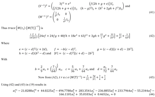
(41)
Thus JE m&"#!$ L&"Τ$MN n is
! !@0
!
|•|P¦24E + 24 „ + 48 ℎ + 18E + 63 + 3„ℎ +!r„ + 11§P¨ +!TP+ 1QP3 (42)
Where
E = "J − K$ "J + 2K$, = −I"J − K$ , „ = "J − K$Y"J + K$ − 2I Z, ℎ = "J − K$"I − K$ and |€| = "J − K$ Y"J + K$ − 2I Z
With
I =29 !+ ‚64ƒ7 !
, J =36 5 !+64 and K =7 72 +! 64 7
Now from (A2), J E "&"Τ$N!$ =|•|U +|•|1©+1T+Q1 (43)
Using (42) and (43) in (19) results in
!!!− 21.8288 !!6+ 44.0225 !C− 494.7780 !@+ 283.3541 !‘− 236.8855 !2+ 233.7964 !r− 55.2344 !−
166.1101 !1+ 35.0103 !+ 0.4652 != 0 (44)
Which when solved within Y0, 1Z we get != 0.219614833 and
= 1 − != 0.780385166
Hence the unique A-optimal design is
η"α“$ = 0.219614833η!+ 0.780385166η (45)
Using values of ! and from "44$ in (30) we have;
u
1 0.306911B 0 0
0.306911 0.0275I1+ 0.0884J1 0 0
0 0 0.3069I1 0
0 0 0 0.0886I1
v (46)
the required A-optimal design.
4. Efficiencies of the Designs
The performance of the RSD and WRSD was measured using the D- and A- criterion.
Table 2. Optimal values.
Rotatable Simplex Design (RSD)
Weighted Rotatable Simplex Design (WRSD)
Factors "¬$ - − ® − - − ® −
2 0.1908 2.5295 0.1618 0.0372
3 0.1075 4.3744 0.0258 0.0409
4.1. D - Efficiency
The performance of the WRSD in comparison to the RSD is measured by the D-efficiency which is defined by
"#$ = ¦|S"¯|S"¯$|°$|¨ 4 ±
. Using the D- optimal ∅6"[y"&$$ values
for the two designs from Table 1, the D – Efficiency values are:
Table 3. D – Efficiency values.
Design Factors
Rotatable Simplex Design (RSD)
Weighted Rotatable Simplex Design (WRSD)
D - efficiency
-²žž"³∗$
2 0.1908 0.1618 0.8480
3 0.1075 0.0258 0.24
4.2. A - Efficiency
Similarly the A – optimal ∅N!"[y"&$$ values for the two designs from Table 1 are used to obtain the A – Efficiency
values as ∅∅¶4"·4$ ¶4"·P$=
m4± ¸¹¢OU·4¶4n¶4
m4± ¸¹¢OU·P¶4n¶4 :
Table 4. A – Efficiency values.
Design Factors
Rotatable Simplex Design (RSD)
Weighted Rotatable Simplex Design (WRSD)
A – efficiency
®²žž"³∗$
2 2.5295 0.0372 0.0147
3 4.3744 0.0409 0.0093
From the efficiencies, it is also noted that the WRSD is 98.53% more A - efficient for two factors and 99.07% more
A - efficient for three factors.
5. Conclusion
In this study, we have presented a method for constructing a WRSD. The constructed design has achieved estimation efficiency as shown by the results in relation to their moment matrices. These designs have also proved to be D- and A- optimal.
Appendix
I. Matrices for )3, 2+ RSD A - Optimality
&"#!$ L&"Τ$MN! for )3, 2+ RSD
&"#!$ L&"Τ$MN!=!@!
7 8 8 8
9 18 41B 0 0 41 CI1+!J1 0 0
0 0 4I1 0
0 0 0 !I1:;
; ; <
0€0N! •0N!3 (A1)
Where
€N!= ‚"J − K$ "J + 2K$ "−I"J − K$ $11B
"−I"J − K$ $11 |€|I1+ "J − K$"I − K$J1ƒ
With
|€| = "J − K$ Y "J + 2K$ − 3I Z and •N!= … !
TI1 0
0 !QI1†
(A2)
References
[1] Box, G. E. P., & Draper, N. R. (1959). A basis for the selection of a response surface design. Journal of American Statistical Association, 54, 622-654.
[2] Das, M. N., & Narasimham, V. L. (1962). Construction of rotatable designs through balanced incomplete block designs. Annals of Mathematical Statistics, 33(4), 1421-1439.
[3] Das, R. N. (1997). Robust second order rotatable designs: Part I RSORD. Calcutta Statistical Association Bulletin, 47, 199-214. [4] Das, R. N. (1999). Robust Second Order Rotatable Designs: Part - II RSORD. Calcutta Statistical Association Bulletin, 49, 65-76. [5] Otieno-Roche E., Koske J. & Mutiso J. (2017). Construction
of Second Order Rotatable Simplex Designs. Manuscript submitted for publication.
[6] Panda, R. N., & Das, R. N. (1994). First order rotatable designs with correlated errors. Calcutta Statistical Association Bulletin, 44, 83-101.
[7] Rajyalakshmi, K., & Victorbabu B. R. (2014). Construction of second order rotatable designs under tri-diagonal correlation structure of errors using central composite designs. Journal of Statistics: Advances in Theory and Applications, 11(2), 71-90.
[8] Rajyalakshmi, K., & Victorbabu, B. R. (2011). Robust Second Order Rotatable Central Composite Designs. JP Journal of Fundamental and Applied Statistics, 1(2), 85-102.
[9] Tyagi, B. N. (1964). Construction of second order and third order rotatable designs through pairwise balanced designs and doubly balanced designs. Calcutta Statistical Association Bulletin, 13, 150-162.
[10] Victorbabu, B. R., & Rajyalakshmi, K. (2012). A new method of construction of robust second order rotatable designs using balanced incomplete block designs. Open Journal of Statistics, 2(2), 88-96.