Impact of Measurement Errors on Estimators of Parameters of a Finite Population with Linear Trend Under Systematic Sampling

(1)

http://www.sciencepublishinggroup.com/j/ajtas doi: 10.11648/j.ajtas.20170606.12

ISSN: 2326-8999 (Print); ISSN: 2326-9006 (Online)

Impact of Measurement Errors on Estimators of Parameters

of a Finite Population with Linear Trend Under Systematic

Sampling

Oloo Odhiambo Erick

*

, James Kahiri, Wafula Mike Erick

Department of Statistics and Actuarial Science, Kenyatta University (KU), Nairobi, Kenya

Email address:

[email protected] (O. O. Erick) *_{Corresponding author}

To cite this article:

Oloo Odhiambo Erick, James Kahiri, Wafula Mike Erick. Impact of Measurement Errors on Estimators of Parameters of a Finite Population with Linear Trend Under Systematic Sampling. American Journal of Theoretical and Applied Statistics. Vol. 6, No. 6, 2017, pp. 270-277. doi: 10.11648/j.ajtas.20170606.12

Received: September 17, 2017; Accepted: October 4, 2017; Published: November 10, 2017

Abstract:

The study involves investigating the impact of measurement errors on estimators of parameters of a finite population with linear trend among population values, under systematic sampling. The study provides deep understanding on the amount and nature of deviation introduced by errors and how these errors affect estimators of parameters of a population with linear trend. Consideration is given to measurement errors that assume a normal distribution. Systematic sampling technique is used where a sample of size n is selected randomly from a finite population with a fixed interval a. Systematic sampling is considered instead of simple random sampling in this case because of its effectiveness in dealing with linear trend. The explicit values of population totals, means and variances together with their estimates are derived. The results indicate that there can be overestimate of the population mean if the expected systematic errors tend towards positive values and underestimate if the expected systematic error tend towards negative values. When random errors are considered, there is no effect on estimated population parameters.

Keywords:

Finite Population with Linear Trend, Systematic Sampling, Measurement Errors

1. Introduction

In an ideal situation, it is assumed that through some kind of probability sampling, in this case systematic sampling, the observation yi on the ith unit is the correct value for that

unit, and that sampling errors may arise solely from the random sampling variation that is present when n_{units are}

measured instead of complete population of N units. Contrary to the assumption, non-sampling errors that are due to measurement or observation do occur at data collection stage.

The true score theory is a good simple model for measurement. It consists of true value and two error components; random error and systematic error.

r s

y= + +t e ε (1)

Where,

y is the measured value t is the true value

r

e is the random error

s

ε is the systematic error

Random error is caused by unpredictable fluctuation in the reading of a measurement apparatus or experimenter’s interpretation of the instrumental reading. Systematic error is caused by any physical factor that affect an experiment or measurement of the variable across the sample in a predictable direction.

(2)

account of measurement error and in devising procedure that corrects such error.

In recent years, a number of papers have examined the consequences of non-classical measurement errors in labor economics.

[4-6], all noted that non-classical measurement errors of the type typically found in income data, attenuates the role of white noise measurement error in models of earnings dynamics.

Measurement errors can best be studied if the true value is obtained. This approach is limited to items for which a feasible method for finding the true value exists. For instance majority of studies using Body Mass Index(BMI) rely on self-reported measures from survey data sets. However Conor et al shows that there is a large body of evidence which suggests that self-reported BMI tends to underestimate true BMI; this occurs both because people underreport their weight and overestimate their height [7]. Looking at measurement errors in self-reported BMI specifically, Plankey et al examines the consequences of these errors when classifying people according to obesity status [8]. Stommel et al [9] compared self-reported and recorded BMI using US data and found a substantial amount of misclassification of obesity status when using self-reported BMI, particularly in the extreme (overweight or underweight) categories. Consequences of this measurement errors were examined when analysing the impact of BMI on a range of health risks. Belloc [10], compared data on hospitalization as reported in household interviews with the hospital records for the individuals. Hospital record produces the true values which are then compared to the observed values from household interviews. Gray [11] compared employee's statements of sick leave with the personal office records. The comparison of data was to determine the presence of measurement errors if any. [12-13] compares respondents’ illness with either doctors’ records on the respondents or with the results of a complete medical examination.

According to Särndal measurement errors arise during data collection stage, and may have a considerable impact on the estimates [14]. In recent studies; Nyabwanga [15] studied Effect of measurement errors on population in random order. Rosella et al [16] studied the influence of measurement error on calibration, discrimination and overall estimation of risk prediction model. O'Neil et al [17] examined the consequences of measurement errors in self-reported BMI when estimating the relationship between obesity and income. Subramani et al [18] studied Estimation of Populations Means in the Presence of Linear Trend among population values under circular systematic sampling. Ouko et al [19] studied the effects of Measurement Errors on Population Estimates from Samples Generated from a Stratified Population through Systematic Sampling Technique. Grellety et al [20] examined the Effect of random error on diagnostic accuracy illustrated with anthropometric diagnosis of malnutrition.

In this project further study is based on The Impact of Measurement Errors on Estimators of Parameters for a finite Population with Linear Trend under Systematic Sampling.

Finite population with linear trend consists of N units identified by the label 1, 2,..., N ordered in increasing size. Through systematic sampling, the population is then divided into a_{samples of}n_{units each.}

The table below shows sets of all possible samples.

Table 1. Sets of all possible samples.

Samples, s

s1 s2 ... sh ... sa

y values

y1 y2 ... yh ... ya

ya+1 ya+2 ya+h y2a

... ... ... ... ... ...

y(n-1)a+1 y(n-1)a+2 y(n-1)a+h yna

Sample totals ts1 ts2 ... tsh ... tsa

Let systematic sampling be denoted as SY.

The sets of all possible samples denoted Ssy consists of a

different sets that are non-overlapping that can be obtained as

Ssy =(s1..., si..., sa) (2)

Sampling design of SY is thus given as

( )

01

sy

if s belongs to S a

otherwise

p s = 

Each sample or a cluster is selected with probability 1a

and observed completely as per the design.

2. Parameter Estimation

2.1. Estimation of Parameters for a Finite Population with Linear Trend Under Systematic Sampling

Let N be the size of a finite population. Suppose the finite population is such that the observed values assume a hypothetical trend as

i

y = +µ βi (3) where µ and β are constants and i=1, 2,...N are ordered in increasing size of the label

The population is then said to possess linear trend among its values.

Let population size N be a multiple of n, N=an. The estimate of population mean under linear systematic sampling in which case a single random start is taken is obtained. as

(

)

1

2

N i i N i

Y y

N

i

N N

µ β

=

= +

+ = +

∑

(4)

According to Mukhopadhyay [20], population with linear trend has a systematic sample given by

( )

1

r l a

(3)

1,...,

l= n

The sample total

( )

{

}

1 1

n s _i

t µ β r l a

=  

=

∑

+ _ + − _ (5) Then the sample mean is written as

1 2

s

n y = +µ βr+a − 

  (6)

y is the mean of a systematic sample and through probability sampling, it is the unbiased estimator of _Y

Similarly, population total is denote as tθ =

∑

_Uyi

Since the interest is in estimating population total, from a design-based approach, Horvitz-Thompson estimator, HTE, Horvitz and Thompson [22] is used.

The estimator is defined as,

i i i s U i i y I y tπ π π =

∑

=

∑

ɵ ₍₇₎

Where π_i _≻0 is the first order inclusion probability. Under Systematic Sampling, SY design with sampling interval a_{, and the response variable} y_i, the population total estimator for _i p I

(

_i 1

)

1

a

π = = = is given as

i s

s i

y

tπ at

π

=

∑

=

ɵ (8)

Where i p I

(

i 1

)

1

a

π = = = is the probability that the th

i

unit of the population is included in the sample. Finite population variance is given as

(

)

(

)

2 2 1 2 1 1 1 12 N i i

S y Y

N N N β = = − − + =

∑

Variance of mean from a simple random sample is given as

( )

(

)(

)

2 2 1 1 12 ran

N n s V y N n a na β − = − + =

Under systematic sampling, the variance of mean is given as

( )

2 1 2

12

sy

a

Var y = −

β

(9)

According to Daroga et al [23], for removing effect of linear

trend, systematic sampling is much more efficient than simple random sampling.

2.2. Estimation of Variance from a Single Systematic Sample

According to Särndal [14], a major drawback of SY is that there is no unbiased estimator for the variance of the estimator of population mean except for some cases of circular systematic sampling. This is because SY is equivalent to cluster sampling with only one cluster selected.

However, under some assumptions about the nature of the population, it is possible to propose estimators that are approximately unbiased for the design variance.

In this case, the appropriate variance estimator for the population with linear trend in which case values of the units are steadily increasing by a constant amount is considered.

Many biased estimators have been proposed for this kind of population;

Wolter [22], made analytical studies on population with linear trend and proposed the following estimator for the variance of the estimator of population total.

Assume n=2m. Since a systematic sample can be looked upon as grouping the population in m groups and choosing 2 units from each group of size 2a, an estimator of the mean of the gth group is

2 1 2

, 1,... 2

i i g g

y y

y = − − g= m

with the variance estimator

2 2 1 2

1

2

i g i g

y y a v a − −   − = _ _  

Hence estimator of Vsy

( )

tɵπ is

(

)

2 1

2

2 ₂

1 ₂ ₁ 2 1 2

1 1 , m g g n

i g i g g

v N V y

m

f n

v N y y f

N

n = −

  =     − = − =

∑

(10)

Cochran [25], suggested the estimator below to be appropriate

( )

₂ ₁2

(

₍

1

₎

2

)

2 2

2

1 '

6 2

n

i i i

i y y y

a n v V t N

a n n

π − + + = − + − = = −

∑

ɵ for

1≺i≤ −n 2

Where

(

)

(

)

2

1 2

2 1 2

6 2

n

i i i i

syl

y y y

S n − + + = − + = −

∑

is the variance of a

(4)

a is the sampling interval.

The estimate is based on successive quadratic terms in the sequence yi. The factor 6 is the sum of squares of the

coefficients in the n−2 differences. The term n₂'

n is the

sum of squares of the weights in y_swy.

'

n is due to the weight 2

₍

₎

1

2 1

r a n a

− −

− applied to the first and the last sample values.

Unless n_{is small,}

2

'

n

n can be replaced by the factor

1

n.

Thus

( )

₂ ₁2

(

₍

₎

1 2

)

2

2 1

,

6 2

n

i i i

i y y y

a v V t N

an n

π

−

+ +

= − +

−

= =

−

∑

ɵ (11)

for 1≺i≤ −n 2

Yates [26], suggested the following estimator among others based successively on second and higher order differences.

(

)

2 4

3 ₁ 1 2 3

1

3.5 4 2 2

n _i _i

i i i i

y y

f

v N y y y

n n

− ₊

+ + +

=

−  

= ₋  − + − + 

 

∑

(12)

The sum of squares contains (n-4) terms.

2.3. Population Total Estimator and Its Variance in Presence of Random Errors

Through measurement procedure, the th

i individual observed is accompanied by the random error term ei.

The observed value is thus given as

i

y = +µ βi e+ (13)

The model can thus be expressed as

i i

y = +µ e (14)

Where

i

y - is the observed value for the _ith_individual,

i

µ β+ =µ - is the true value for the th

i individual,

i

e - is the random error for the _ith_individual.

For the true function value µi, population total is

i

t_θ =

∑

µ

Define

1

N _{i i} _s i s i

i i

y I y

tπ

π π

=

∑

=

∑

ɵ as the population total

estimator (Horvitz-Thompson estimator), with π_i ≻0

In SY design, π_i = p I

(

_i= =1

)

1_a

The joint expectation of the population total estimator is

obtained as;

( )

pm p m _U i

E tɵπ =E __E ɵtπ s __=

∑

µ

The total variance of tɵπ with respect to sampling design

( )

.

p and the measurement model m_{according to Särndal}

[14] is given as

( )

pm p m p m

V ɵtπ =E __V tɵπ s __+V __E tɵπ s __ (15) The variance of population estimator is the sum of the expected value of the conditional variance and the variance of conditional expected value.

Therefore total variance consists of measurement variance and sampling variance respectively.

Measurement variance when decomposed is expressed as follows;

( )

2

p m _U i ij

i j

E V tπ s a δ a δ

≠

 ₌ ₊  

 ɵ 

∑

∑∑

Sampling variance when decomposed is also expressed as

( )

(

1

)

p m i j

ij

V __E ɵtπ s __=

∑∑

a− µ µ

Combining the results we have

( )

2

(

₁

)

pm _U i ij i j

i j ij

V tπ a δ a δ a µ µ

≠

=

∑

+

∑∑

+

∑∑

−

ɵ

(16)

This is the derived equation for total variance in presence of random error with respect to sampling design p

( )

. and measurement model m_jointly.

The measurement variance

2

i ij

U

i j

a δ a δ

≠

+

∑

∑∑

_has

simple response variance and the correlated response variance as its components respectively.

(

1

)

_i _j

ij

a− µ µ

∑∑

_{is the sampling variance. Simple}

response variance reflects the random variation in a respondent’s answer to a survey over repeated measurements. Correlated response variance also known as interviewer variance occurs because response errors are correlated for sample units interviewed by the same interviewer.

2.4. Mathematical Model for Errors of Measurement

Suppose measurement could be independently repeated many times on unit i∈s, we could generate different yi

-values.

Let yi be the realized value in the repeated observation,

then

i i i

(5)

Let µ β+ i=µ_i

Thus

i i i i

y =µ + +e ε (17)

i

µ is the true value of unit i

Both ei and εi are random variables where e ii

(

∈s

)

are independent random variables with E e

(

i =0

)

and varianceδe2.

1,... a

ε ε are independent and identically distributed random variables with the expected value ε and variance δ_ε2

The random variables εi

(

i=1,...a

)

are independent of the random variables e ii

(

∈s

)

From the selected sample consisting of yi-values, the first

and second-order moments are;

(

)

( ) ( ) ( )

(

)

(

)

(

)

2 2 2

,

m i i i i i i

m i e i

m i m i j ij

E y s E E e E

V y s

Cov y s C

ε

µ ε µ ε α

δ δ δ

ε ε δ

= + + = + =

= + =

= =

i

ε is the systematic error on the individual measured value and E

( )

εi =ε is the bias in measurement.

Unlike random error, systematic error tend to be consistently either positive or negative - because of this, systematic error is sometimes considered to be bias in measurement.

2.5. Measurement Bias and Expectation of π-estimator

Measurement bias arises when expected measurement value on elements do not agree with true element values.

( )

pm pm

B tɵπ =E tɵπ −t_θ

The derived expected measurement value is expressed as

( )

pm

U

E tɵπ s = +tθ

∑

ε

The derive total measurement bias with respect to sampling design p

( )

. and measurement model m respectively is thus expressed as follows

( )

pm

U U

B tɵπ = +tθ

∑

ε− =tθ

∑

ε (18)

2.6. Decomposing Variance of Population Total Estimator When Systematic Errors Are Present

According to Särndal [14] the total variance of tɵπ with respect to sampling design p

( )

. and the measurement model

m is given as

( )

pm p m p m

V ɵtπ =E __V tɵπ s __+V __E tɵπ s __ (19) Measurement variance when decomposed is expressed as follows;

( )

2

p m _U i ij

i j

E V tπ s a δ a δ

≠

 ₌ ₊  

 ɵ 

∑

∑∑

(20)

Similarly, sampling variance is decomposed as follows

( )

(

)

(

)

( )

p m p m _s i

m _s i _s m i _s i

V E t s V E a y

E a y a E y a

π α    ₌         = =

∑

ɵ Now

(

)

( )

(

( )

)

(

( ) ( )

)

(

)

(

)

(

)

(

)

(

)

(

)

(

)

2 ₂

2 2 2

2 2 2 2 2 2 , cov 1 1 1 1 1 1

p m _s i p _s i

i p i i j i j

U i j

i i i ij i j i j

U i j

i i j

U i j i i j U i j

i j i j

V E a y V a

a V I s a I s I s

a a

a a a a

a a

a

α

α α α

π π α π π π α α

α α α

α α ≠ ≠ ≠ ≠  ₌         = + = − + − − − = + = − + − = −

∑

∑∑

∑

∑∑

∑

∑∑

∑

∑∑

( )

_,

(

1

)

p m _{i j} i j

V __E ɵtπ s __=

∑∑

a− α α

Combining the results the total variance becomes

( )

2

(

)

,

1

pm _U i ij i j

i j i j

V tπ a δ a δ a α α

≠

=

∑

+

∑∑

+

∑∑

−

ɵ

(21)

We let α_i =µ ε_i+ _k and α_j =µ_j+ε_l Substituting 17 &18 into 16 above

( )

(

)(

)

(

)

(

)

(

)

2 , 2 , 1 1

pm _U i ij i k j l

i j i j

i ij i j i l j k k l

U i j

i j

V t a a a

a a a

π δ δ µ ε µ ε

δ δ µ µ µ ε µ ε ε ε

≠ ≠ = + + − + + = + + − + + +

∑

∑∑

∑

∑∑

ɵ

( )

2

(

)

( )

(

)

(

)

, ,

1 1

pm _U i ij _{i j} i j _{i j} i l j k k l

i j

V tπ a δ a δ a µ µ a µ ε µ ε ε ε

≠

=

∑

+

∑∑

+ −

∑∑

+ −

∑∑

+ +

ɵ

(22)

(6)

3. Numerical Results and Discussion

A finite population of size N is generated for a population without errors, a population with random errors and a population with systematic errors.

The population total variances, the population means and the population totals are then computed.

In the selection of a systematic sample of size n_{, a random}

start r is selected between 1 and a_{inclusive in which case} a_{is the sampling interval.}

To estimate parameters, simulation of data is done 10 times in each case the estimate is obtained. The results are then averaged to get the estimates of all parameters required in the study.

Estimation of variance is done using the three estimators

below simplified to reflect systematic sampling.

(

)

2

(

)

2

1 1 ₁ 2 1 2

n

i g i g g

v a a y ₋ y

=

= −

∑

− (23)

(

)

(

₍

₎

)

2 2

1 2

2 1

6 2

n

i i i i y y y

v N a

n

−

+ +

= − +

= −

−

∑

for

(

1≤ ≤ −i n 2

)

(24)

( ) ₍ ₎

2 4

4

1 2 3

1 3

2 2

1

3.5 4

n

i i

i i i

i

y y

y y y v N a

n

− ₊

+ + +

=

 ₋ ₊ ₋ ₊ 

 

 

= −

−

∑

for (1≤ ≤ −i n 2)₍₂₅₎

The tables from case 1 to case 3 consists of parameters and their estimates for populations without errors and populations with errors.

Case 1

Let N=800, n=32, a=25

Table 2. Population Parameters and Their Estimates for er∼N( )0,1 and εi∼N(−0.6,1.5 .)

Pop Parameters Estimates

Mean Total Pop.var Estimated mean Estimated total V1 V2 V3

No error 423.525 338, 820 36, 691, 200 422.475 337, 980 25, 412, 184 0 0

With er 423.530 338, 824 36, 716, 492 421.102 336, 880 25, 556, 994 18, 875 18, 956

With εi 422.940 338, 352 37, 594, 498 418.767 335, 013 26, 027, 490 50, 734 52, 305

Table 3. Population Parameters and Their Estimates for er∼N( )0,1 and εi∼N(0.5,1.5 .)

No error 423.525 338, 820 36, 691, 200 422.475 337, 980 25, 412, 184 0 0

With er 423.563 338, 824 36, 883, 067 420.752 336, 601 25, 662, 927 17, 652 18, 720

With εi 424.020 339, 216 36, 740, 158 427.770 342, 216 25, 450, 518 44, 746 37, 078

From tables 2 & 3, the results shows that:

1. The population mean is underestimated if a population with systematic errors has a negative systematic bias.

2. The population mean is overestimated if a population with systematic errors has a positive systematic bias.

3. Population mean in presence of random errors almost

conforms to the mean of population without errors.

4. Estimators of variance of population total estimator underestimate the population total variance.

5. v2 and v3 for population with true values are zeros

but very small values for population with errors.

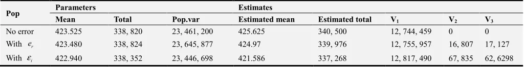
Case 2

Let N=800, n=40, a=20

No error 423.525 338, 820 23, 461, 200 425.625 340, 500 12, 744, 459 0 0

With er 423.480 338, 824 23, 645, 877 424.97 339, 976 12, 755, 957 16, 807 17, 127

With εi 422.940 338, 352 23, 446, 698 421.586 337, 268 12, 817, 490 67, 835 62, 6298

No error 423.525 338, 820 23, 461, 200 426.938 341, 550 12, 744, 459 0 0

With er 423.545 338, 824 25, 514, 150 420.900 336, 720 12, 706, 411 17, 792 18, 229

(7)

1. The population mean is underestimated if the expectation of systematic errors is negative.

2. The population mean is overestimated if the expectation of systematic errors is positive.

3. Estimates from v1 for population with systematic errors

exceeds the corresponding estimates from the population without errors.

4. Estimates from v1 exceeds estimates from v2 and v3.

5. The mean of population with random errors is closer to the actual population mean.

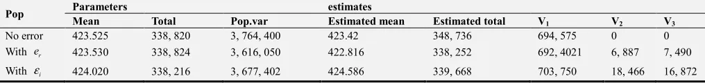
Case 3

Let N=800, n=100, a=8

No error 423.525 338, 820 3, 764, 400 422.77 338, 216 694, 575 0 0

With er 423.230 338, 824 3, 663, 845 423.589 338, 871 698, 297 6, 509 6, 787

With εi 422.940 338, 352 3, 680, 080 422.702 338, 161 723, 733 19, 702 19, 937

Pop Parameters estimates

No error 423.525 338, 820 3, 764, 400 423.42 348, 736 694, 575 0 0

With er 423.530 338, 824 3, 616, 050 422.816 338, 252 692, 4021 6, 887 7, 490

With εi 424.020 338, 216 3, 677, 402 424.586 339, 668 703, 750 18, 466 16, 872

1. When the sample size is increased, both the population variances and estimated variances are reduced.

2. Estimates from v1 are much higher than the respective

estimates from v2 and v3.

3. Positive expected systematic errors overestimate population means and totals while negative expected systematic errors underestimate population means and total.

4. Summary

From the study, it is observed that:

1. The population means and hence the population totals are overestimated for the case where expectation of systematic errors is positive.

2. The population means and hence the population totals are underestimated for the case where expectation of systematic errors is negative.

3. Impact of random errors on population mean and population total is minimal and inconsistent.

4. The variances of population total estimator are all underestimated using the three estimators, v1, v2 and v3.

5. Increase in sample size leads to decrease in estimated variance of population total estimator.

6. For population with systematic errors, the estimated variances are over represented. Estimator v1 gives

higher variance than estimators v2 and v3.

5. Conclusions

The study has shown that:

Impact of random errors on population mean, population

total and estimated variance of population total estimator is very minimal.

Systematic errors produces systematic bias that overestimate the population mean when the bias is positive and underestimate the population mean when the bias is negative.

All the three estimators underestimate population variances and therefore they are biased. Among the three, v1 is better

because it gives values closer to the population variance. Generally systematic errors lead to over representation of the estimated variance while random errors have no impact on estimates of population variance.

References

[1] Fuller, W. (1987). Measurement Error Models. Wiley and Sons.

[2] Carroll, R., J, R. D. and Stefanski, L. (1994). Measurement Error in nonlinear models, Chapman and Hall, London. [3] Bound, J., Brown, C., and Mathiowetz, N (2001).

Measurement Error in Survey data. American Journal of Theoretical and Applied Statistics, 5.

[4] Pischke, J. (1995). Measurement error and earnings dynamics: some estimates from the psid validation study. Journal Business of Econmics Statistics, 13(3):305-314.

[5] O’ Neil, D., Sweetman, O., and Van der gaer, D. (2007). The effects of measurement error and omitted variables when using transition matrices to measure intergenerational mobility.

Journal of Economic Inequality, 5(2):159-178.

(8)

[7] Conor, G., Temblay, M., Moher, D., and Gorver, B. (2007). A comparison of Direct vs Self-reported Measures for Assessing Height, Weight and Body Mass Index: a systematic review.

Obesity Rev. 8:307-326.

[8] Plankey, M., Stevens, J., Flegal, K., and Rust, P. (1997). Prediction equations do not eliminate systematic error in self-reported body mass index. Obesity Research, 5(4):308-314.

[9] Stommel, M. Schoenborn, C. (2009). Accuracy and usefulness of BMI measures based on self-reported weight and height: findings from the nhanes and nhis 20012006, BMC Public Health, 9(421).

[10] Belloc, N. (1954). Validation of morbidity survey data by comparison with hospital records, Journal of American Statistics Associations, 49:832-846.

[11] Gray, P. (1955). The Memory Factor in Social Survey. Journal of American Statistics Associations, 50:344-363.

[12] Sagen, O. K, D. R and Simmons, W (1959). Health Statistics from record sources and household interview compared.

Proceedings of the social Statistics election of American Statistics Associations, pages 6-15.

[13] Trusell, R and Elinson, J. (1959). Chronic Illness in a Large City. Harvard University Press Cambridge Mass.

[14] Särndal, C. (1992). Model assisted Survey Sampling. Springer-verlag New York, Inc, USA.

[15] Nyabwanga, R. (2010). Effect of measurement errors on population in random order when sampling systematically. Unpublished project department of Mathematics Kenyatta University.

[16] Rosella, L. C. Corey, P. Stukel, T. Mustard, C. Hux, J. and Manuel, D. G. (2012). The influence of measurement error on

calibration, discrimination and overall estimation of a risk prediction model. Population Health Metr; 10:20. doi:10:1186/1478-7954-10-20. [PMC 3545925].

[17] O’ Neil, D. and Olive, S. (2013). The consequences of measurment error when estimating the impact of obesity on income. IZA Journal of Labor Economics, 2(3).

[18] Subramani, J. and Singh, S. (2014). Estimation of population mean in the presence of linear trend. Communications in the Statistics-Theory and Methods, 43.

[19] Ouko, A., Cheruiyot, W., and Emily, K. (2014). Effects of measurement errors on population estimates from samples generated from a stratified population through systematic sampling technique. Expert Journal of Economics, 2:120-132. [20] Grellety, E. Golden, M. H (2016). The effect of Random error

on diagnosis accuracy illustrated with the anthropometric diagnosis of malnutrition. PLoS ONE 11(12): e0168585 doi 10.1371.

[21] Mukhopadhyay, P. (1998). Theory and Methods of Survey Sampling. Prentice-Hall of India Private Ltd.

[22] Horvitz, D. and Thompson, D. (1952). A generalization of Sampling Without Replacement From a Finite Universe.

Journal of American Statistics Associations, 47:663-685. [23] Daroga, S. and Chaudhary, F. S (1986). Theory and Analysis of

Sample Survey Designs. New Age Inernational (P) Ltd. [24] Wolter, K. (1985). Introduction to Variance Estimation,

Springer-Verlag, New York.

[25] Cochran, W. G. (1977). Sampling Techniques, John Wiley and Sons, third edition.