Generalized Difference Formula for a Nonlinear Equation

(1)

Published online July 30, 2014 (http://www.sciencepublishinggroup.com/j/acm) doi: 10.11648/j.acm.20140304.14

ISSN: 2328-5605 (Print); ISSN: 2328-5613 (Online)

Generalized difference formula for a nonlinear equation

Hamideh Eskandari

Department of Mathematics, Payame Noor University, I. R. Iran

Email address:

[email protected]

To cite this article:

Hamideh Eskandari. Generalized Difference Formula for a Nonlinear Equation.Applied and Computational Mathematics. Vol. 3, No. 4, 2014, pp. 130-136. doi: 10.11648/j.acm.20140304.14

Abstract: In this paper, a new iteration scheme is proposed to solve the roots of a nonlinear equation. It is the purpose of

this paper to show that, although the new iteration method seems to be of high convergence, the results are promising in that it requires more computation work and even be divergent. In here, we use iteration method that applied derivatives of the first order and the second order; we substitute difference formulas in iteration formulas. This method cause that our iteration method have not any derivative formulas.

Keywords: Newton Method, Hybrid Method, Halley Iteration, Steffenson Method

1. Introduction

One of the most important problems in Numerical Analysis is finding different values of the

x

variable in the

( ) 0

f x = equation. Among the methods, iteration methods are very popular and are used by many researchers. Bisection method, fixed point iteration, secant method and … [1] – [3] and [8] – [10] are among various methods used for solving these problems.

1.1. Fixed Point Method

In this section [10] a completely general framework for finding the roots of a nonlinear function is provided. The method is based on the fact that, for a givenf :[ , ]a b →R, it is always possible to transform the problem f x( )=0into

an equivalent problemx −ϕ( )x =0, where the auxiliary function ϕ:[ , ]a b →R has to be chosen in such a way that

( )

ϕ α =α wheneverf( )α =0. Approximating the zeros of a

function has thus become the problem of finding the fixed points of the mapping

ϕ

, which is done by the following iterative algorithm:

Givenx₀, letxn+₁=ϕ(xn). We say that this formula is a

fixed-point iteration and

ϕ

is its associated iteration function. Sometimes, this formula is also referred to as functional iteration for the solution of ( )f x =0.

The choice of

ϕ

is not unique.

1.2. The Bisection Method

The simplest method is that of bisection [8] – [10]. The following theorem, from calculus class, insures the success of the method. The bisection method is based on the following property: [1]

Theorem (Intermediate Value Theorem):

Given a continuous function f : [ , ]a b →R , such that f a f b( ) ( )<0, then ∃ ∈α ( , )a b such that f( )α =0.

Assume that f x( ) is continuous on given internal [ , ]a b and that is also satisfiesf a f b( ) ( )<0.

Using the Intermediate Value Theorem, the function ( )

f x must have at least one root in[ , ]a b . Usually [ , ]a b is

chosen to contain only one root

α

, but for the bisection method will always converge to some root

α

in [ , ]a b , because off a f b( ) ( )<0.

Bisection Method Theorem:

If f x( ) is a continuous function on

[ , ]

a b

such that f a f b( ) ( )<0; then after

n

steps, the algorithm run bisection will return

c

such that

2n

b a

c− ≤

α

− where

α

is some root of ( )f x .In particular, the Intermediate Value Theorem tells us that if

f x

( )

is continuous and we know

, b

a such that f a( ) , f(b)have different sign, then there is some root in [ , ]a b . A decent estimate of the root is

2

(2)

- f a( ) , ( )f c have different signs. -

f c

( ) , ( )

f b

have different signs.

We now choose to recursively apply bisection to either [ , ]a c or [ , ]c b , respectively, depending on which of these two options hold.

Table AI. Newton Method

n xn _{f xn}( )

0 1 5.

1 0.500000000000000 0.75000000000000 2 0.392857142857143 0.03443877551020 3 0.387439807383628 0.00008804257090 4 0.387425886814712 _5.8135*10−10

Table AII. Hybrid Method

n xn f x( n)

0 1 0.47213595499958

1 0.47213595499958 0.55728090000842 2 0.38957898648928 0.01363130609916 3 0.38742735070977 0.00000925907305 4 0.38742588672347 _4.28*10−12

5 0.38742588672280 _4.*10−14

6 0.38742588672280 _4.*10−14

1.3. Newton's Method

Suppose that an initial approximation

x

₀is known for the favorite root

α

of ( ) 0f x = .

Newton's method [8, 9, and 10] will produce a sequence of iterates

{

x_n:n≥1

}

, which we hope will converge to

α

. Since

x

₀ is assumed near to

α

, approximate the diagram of y =f x( )in the near of its root

α

by constructing its tangent line at

0 0

(x , (f x )). Then use the root of this tangent line to approximate

α

; call this new approximation

x

1. Repeat this process, ad infinitum, to obtain a sequence of iterates

x

_n.

Table AIII(1). Omega Method ω=0

n xn f x( )n

0 1 5.

1 0.387425886722793 0. 2 0.387425886722793 0.

Table AIII(2). Omega Method ω=0.4

n xn f x( n)

0 1 5.

1 0.48402626637237 0.63894934510461 2 0.39072414994510 0.02089268383136 3 0.39072414994510 0.00002604334567 4 0.38742588672920 4.952*10−11 5 0.38742588672278 -8.* 10−14

6 0.38742588672279 -2.* 10−14

7 0.38742588672279 -2.* 10−14

Table AIII(3). Omega Method ω=0.85

n xn f x( )n

0 1 5.

1 0.54372016956833 1.06177554665956 2 0.40322463714952 0.10066887261117 3 0.38762217132268 0.00124152839345 4 0.38742591778091 1.9642878*₁₀−7 5 0.38742588672279 _-2.*10−14 6 0.38742588672279 -2.* 10−14

Theorem:

Assumef x( ), f′( )x and f′′( )x are continuous for all

x

in some neighborhood of

α

, and assume

( ) 0

f α = ,f ′( )α ≠0. Then if

x

₀ is chosen sufficiently close to

α

, the iterate

{

xn:n≥1

}

of (1) will converge to

α

. Mostly this equation of f x( )=0 is solved by the Newton iteration method [1, 2, 3], that is

n

n 1 n

n

f (x )

x

f (x )

+

=

−

_′

(1)

Table AIV. Steffenson Method

n

x

_n f x( )_n

0 1 5.

1 0.800000000000000 3.12000000000000 2 0.628193832599119 1.69665780434319 3 0.496252017034795 0.72380626137249 4 0.417138263704964 0.19056604796024 5 0.390201335144078 0.01757658642097 6 0.387452389650257 0.00016762133812 7 0.387425889162957 1.543295*10−8

8 0.387425886722793 0. 9 0.387425886722793 0.

Table AV. Halley Method

n x_n f x( )_n

0 1 5.

1 0.411764705882353 0.15570934256055 2 0.387429020918857 0.00001982242586 3 0.387425886722793 0.

4 0.387425886722793 0.

Table AVI. New Method

n xn f x( n)

0 1 5.

1 0.387425886722793 0.

It is known that Newton method has the convergence of the second order term.

For obtaining of Newton formula, we can write

2

1

( ) ( ) ( )( ) ( )( )

2

n n n n n

(3)

Where

x

_n is the nth approximation to the root of equationf (x)=0.

We eliminate terms of two orders in Taylor expansion, so we havef x( )=f x( n)+f ′(xn)(x −xn).

And if we assume that

α

is root of equation thus

( )= ( n)+ ′( n)( − n)=0

f α f x f x α x . So

( ) ( ) − = −

′

n n

n

f x x

f x

α . And thus we obtain Newton

formulax_{n 1} _xn f (x )n f (x )_n

= −

+ _′ .

Table BI. Newton Method

n

x

f x( )_n

0 1 -0.632120558828558

1 0.812309030097381 -0.092166771534312 2 0.774276548985500 -0.003144824978613 3 0.772884756209622 -0.000004050085548 4 0.772882959152202 -6.743*10−12

5 0.772882959149210 0. 6 0.772882959149210 0.

Table BII. Hybrid Method

n

x

_n f x( n)

0 1 0.801305391412735

1 0.801305391412735 -0.065767646830858 2 0.773375282149370 -0.001110066508433 3 0.772883108807310 -3.37288151*10-7 4 0.772882959149220 -2.2*10−14

5 0.772882959149210 4.* 10−14 6 0.772882959149210 _4.* 14

10−

1.4. The Secant Method

Since with Newton's method, the graph of y= f x( ) is approximated by a straight line in the near of the root

α

. In this method, assume that

x

₀ and

x

₁ are two initial estimates of the root α . Approximate the graph of

( )

y

=

f x

by the secant line determined by ( , ( ))x f x₀ ₀

and( , ( ))x f x₁ ₁ . Let its root be denoted by

x

2; we hope it will be an improved approximation of

α

.

Table BIII(1). Omega Method ω=0

n

x

_n f x( )_n

0 1 -0.632120558828558

1 0.766860964862945 0.013496437197406 2 0.772883063543665 _-2.35276347* 7

10− 3 0.772882959149210 0.

4 0.772882959149210 0.

Using the slope formula with the secant line, we have

1 0 1

1 0 1 2

(

)

(

)

(

) 0

f x

x

−

₌

−

Solving for

x

₂

1 0

2 1 1

1 0

(

)

(

)

(

)

x

f x

−

=

−

⋅

−

Table BIII(2). Omega Method ω=0.4

n

x

_n f x( )n

0 1 -0.632120558828558

1 0.806016194968660 -0.077004350315338 2 0.773680808808762 -0.001799462775209 3 0.772883430692041 -0.000001062728024 4 0.772882959149380 -3.83*₁₀−13

5 _{0.772882959149212} _-5.* 15

10− 6 0.772882959149212 -5.* 10−15

Table BIII(3). Omega Method ω=0.85

n

x

_n f x( )n

0 1 -0.63212055882856

1 0.82935332733815 -0.13412020395267 2 0.77741579936104 -0.01025877010286 3 0.77291503982920 -0.00007230315836 4 _{0.77288296076991} _-3.65261* 9

10− 5 0.77288295914921 0.

6 0.77288295914921 0.

Using

x

₁ and

x

₂, repeat this process to obtain

x

₃, etc. The general formula based on this in

1 1

1

(

)

n

1 (

)

(

)

n n

n n n

n n

x

f x

− +

−

=

−

⋅

≥

−

This is secant method. As with Newton's method, it is not guaranteed to converge, but when it does converge, the speed is usually greater than of the bisect method.

Table BIV. Steffenson Method

N xn f x( )n

0 1 -0.632120558828558

1 0.686492189384687 0.179814370679726 2 0.765456817630988 0.016621779460841 3 0.772819746378117 0.000142455819040 4 0.772882954508837 _1.0458122* 8

10−

5 0.772882959149210 0. 6 0.772882959149210 0.

Table BV. Halley Method

n x_n f x( n)

0 1 -0.632120558828558

1 0.777369844446792 -0.010154331975978 2 0.772882993621885 -7.7691909*₁₀−8 3 0.772882959149210 0.

(4)

1.5. Steffenson’s Method

Instead of using differential in iteration formula (1), considering Steffenson’s method formula [1], differential definition can be used in the following way:

f (x f (x)) f (x)

f (x)

+ −

′ = (2)

And by using substitution in (1), we have the following formula can be obtained:

n n 1 n

n n n

n

f (x )

x x

f (x f (x )) f (x ) f (x )

+ = − ₊ ₋

And so:

2 n

n 1 n

n n n

(f (x ))

x

f (x

f (x )) f (x )

+

=

−

₊

₋

(3)

This is an order of quadratic method. Too, Halley iteration [7] is

n n n 1 n

2 n n

n

f (x ).f (x )

x x

f (x ).f (x ) (f (x ))

2 +

′

= − _′′

′ − (4)

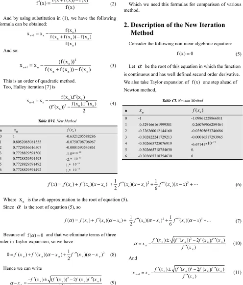
Table BVI. New Method

n x_n f x( _n)

0 1 -0.6321205588286

1 0.8052085081555 -0.0750708706967 2 0.7729536616507 -0.0001593543861 3 0.7728829591500 _-1.8*₁₀−12 4 0.7728829591493 -2.* ₁₀−13

5 0.7728829591492 _1.* ₁₀−13

6 0.7728829591492 _1.* ₁₀−13

And hybrid iteration [4] is

2 1

4 2

+ =− ± −

n

B B AC x

A Where

( )

′′

= n

A f x and

6 (

′

) 2

′′

(

)

=

n

−

n n

B

f

x

f

x

and

C

=

6 (

f x

n

)

−

6 f

′

(

x

n

)

x

n

+

f

′′

(

x

n

)

x

n2.

Which we need this formulas for comparison of various method.

2. Description of the New Iteration

Method

Consider the following nonlinear algebraic equation: f (x)=0 (5)

Let

α

be the root of this equation in which the function is continuous and has well defined second order derivative. We also take Taylor expansion of f (x) one step ahead of Newton method,

Table CI. Newton Method

n

x

_n f x( n)

0 -1 -1.09861228866811

1 -0.529166161999381 -0.26076906289464

2 -0.326260012144160 -0.02505653746686

3 -0.302822241729213 -0.00016517293965

4 -0.302665725076919 _-6.67141*10−19

5 -0.302665718754630 0.

6 -0.302665718754630 0.

2 3

1 1

( ) ( ) ( )( ) + ( )( ) ( )( )

2 6

n n n n n n

f x = f x + f x′ x−x f′′ x x−x + f′′′ x x−x + ⋅⋅⋅ (6)

Where

x

_n is the nth approximation to the root of equation (5). Since

α

is the root of equation (5), so

2 3

1 1

( ) ( ) ( )( ) ( )( ) ( )( ) ...

2 6

n n n n n n

f α = f x +f x′ α−x + f′′ x α−x + f′′′ x α−x + ₍₇₎

Because of f ( ) 0α = and that we eliminate terms of three order in Taylor expansion, so we have

2

1

0 ( ) ( )( ) ( )( )

2

α

′ ′′

=f xn +f xn −xn + f xn −xn (8)

Hence we can write

2

( ) ( ( )) 2 ( ) ( )

( )

n n n n

n

f x f x f x f x x

f x

α− =− ′ ± ′ _′′ − ′′ (9)

And so

2

( ) ( ( )) 2 ( ) ( )

( )

α= − ′ n ± ′ n_′′ − n ′′ n

n

f x f x f x f x x

f x (10)

And

2 1

( ) ( ( )) 2 ( ) ( )

( )

+

′ ± ′ − ′′

= −

′′

n n n n

n n

n

f x f x f x f x x x

(5)

Table CII. Hybrid method

n x_n f x( _n)

0 -1 -0.48746977624315

1 -0.48746977624315 -0.20845898909260 2 -0.311730565520424 -0.00958821656394 3 -0.302680218773610 -0.00001530077621 4 -0.302665718790784 _-3.815* 11

10− 5 -0.302665718754628 _1.* 15

10−

6 -0.302665718754620 _9.* 15

10−

This formula is iteration method and we see it in various books [2]. And too we see it have convergence of three orders. We know that we find roots of equation with any

∆

[5] (where 2

( ′( )) 2 ( ) ′′( ) ∆ = f xn − f xn f xn ).

Now, if we pay attention to formula (3), then we can use from difference formulas too. Thus we can replace both derivatives of first order and second order with difference formula. That is

f (x h) f (x h) f (x)

2h

+ − −

′ ≈

Andf (x) f (x h) 2f (x) f (x₂ h) h

+ − + −

′′ ≈ (whenh→0)

So we will write (because f (x)→0 in roots off (x)=0)

f (x f (x)) f (x f (x)) f (x)

2f (x)

+ − −

′ ≈

2

f (x f (x)) 2f (x) f (x f (x)) f (x)

(f (x))

+ − + −

′′ ≈

Thus we have

n n n n

n

f (x f (x )) f (x f (x )) f (x )

2f (x )

+ − −

′ ≈ ₍₁₂₎

n n n n n

n 2

n

f (x f (x )) 2f (x ) f (x f (x )) f (x )

(f (x ))

+ − + −

′′ ≈ (13)

We will substitute formulas (12) and (13) in formula (11). Therefore we will obtain

1 2 2

1 2

( ( )) ( ( ))

( )

2 ( )

( ( )) ( ( )) ( ( )) 2 ( ) ( ( ))

(

( ( )) 2 ( ) ( ( ))

2 ( ) ( ( ))

2

( )

+

+ − −

 

−

  _ _

+ − −   + − + −

= − ±_ _ ÷_ _

+ − + −  

 

 

n n n n

n

n n n n n n n n n

n n

n n n n n

n n

n

f x f x f x f x

f x

f x f x f x f x f x f x f x f x f x

x x

f x f x f x f x f x

f x f x

f x

(14)

This phrase is iteration method too. Using this equation is very easier than (11), because it hasn’t any derivative formula.

3. Numerical Examples

In this section we perform some numerical examples using our new method and we will compare these results to famous methods. All computations were done MAPLE. We know that an approximate solution rather than the accurate root, depending on the precision (

ε

) of computer. We use the following stopping test for computer programs:

1. xn 1+ −xn <

ε

2. f (xn 1+ ) <

ε

3.1. Example A

Consider this second degree polynomial

3 x

2

+

4 x

− =

2

0

. The exact solutions are -1.72075922005613 and 0.387425886722793.

The obtained results of the Newton method, Hybrid iteration, Omega method, Halley method, Steffenson method and new method [4] and this new iteration are shown in Tables AI, AII, AIII, AIV, AV and AVI order. (_ε₌₁₀−100₎

In order to find a position root x₀ =1 is suggested.

Table CIII(1). Omega Method ω=0

n

x

_n f x( )n

0 -1 -1.09861228866811

1 -0.287266867923168 0.016186774118225

2 -0.302667684021202 -0.00000207379086

3 -0.302665718754634 0.

4 _{-0.302665718754628} _1.* 15

10−

Table CIII(2). Omega Method ω=0.4

n x_n f x( )_n

0 -1 -1.09861228866811

1 -0.50591680972171 -0.23129462452395

2 -0.316927814171480 -0.01510673642993

3 -0.302709710668802 -0.00004642170159

4 -0.302665719153972 -4.2140*10-10

5 _{-0.302665718754647} _-2.* 14

10−

(6)

Table CIII(3). Omega Method ω=0.85

n xn f x(n)

0 -1 -1.09861228866811

1 -0.58623368354393 -0.33675740341608 2 -0.364713041488866 -0.06666789563635 3 -0.304790707442556 -0.00224356642394 4 -0.302667716771138 -0.00000210834930 5 -0.302665718756380 -1.85*10−12

6 _{-0.302665718754621} _8.* 15

10− 7 -0.302665718754634 0.

3.2. Example B

Consider the equation_{f x}_{( )}= −_x3 _e−x=₀

. In order to find a position root close to x=1andx0=1 is suggested. The

obtained results of the Newton method, Hybrid iteration, Omega method, Halley method, Steffenson method and new method [4] and this new iteration are shown in Tables BI, BII, BIII, BIV, BV and BVI order. (_ε₌₁₀−50₎

Table CIV. STEFFENSON METHOD

N xn f x(n)

0 -1 -1.09861228866811

1 -0.605989266652406 -0.36438692984727 2 -0.406650628397178 -0.11337792786986 3 -0.311930734483714 -0.00980046741579 4 -0.302713739561214 -0.00005067317283 5 -0.302665719977280 -1.29017*10−9 6 -0.302665718754625 _4.* 15

10− 7 -0.302665718754629 0.

3.3. Example C

Consider the equation_{f x}_{( )}_{= −}_x _ln(_x4_{+ + =}_{2) 1} ₀_._{In order to}

find a position root close tox= −0.302665718754628 and

0 1

x = − is suggested. The obtained results of the Newton method, Hybrid iteration, Omega method, Halley method, Steffenson method and new method [4] and this new

iteration are shown in Tables CI, CII, CIII, CIV, CV and CVI order. (_ε₌₁₀−13₎

Table CV. Halley Method

N xn f x( )n

0 -1 -1.09861228866811

1 -0.393093790637133 -0.09810890462214

2 -0.302298905285011 0.000387032547151

3 -0.302665718778829 _-2.554*10−11

4 -0.302665718754626 3.* 10−15

5 -0.302665718754629 0.

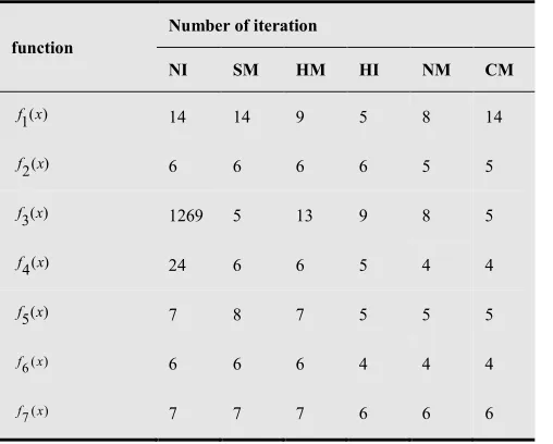
4. Some Equations

We display results for some functions in table D and too we present for some methods. Thus we show that Newton iteration with NI, Steffenson method with SM, Hybrid method [4] with HM, Halley iteration [7] with HI, New method [5] and [6] with NM and current method with CM in tables D and table E.

Table CVI. New Method

n xn f x(n)

0 -1 -1.09861228866811

1 -0.333396491471923 -0.03270218859600

2 -0.302668000254151 -0.00000240748675

3 -0.302665718754642 _-1.* 10−14

4 -0.302665718754630 0.

5. Conclusion

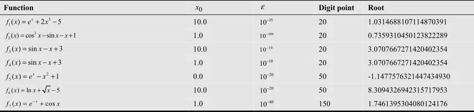
Table D. Test of Functions

Function x0 ε Digit point Root

3 1( )= +2 −5

x

f x e x 10.0 35

10− 20 1.0314688107114870391

3

2( )=cos −sin − +1

f x x x x 1.0 100

10− 20 0.7359310450123822289

3( )=sin − +3

f x x x 10.0 ₁₀−10 ₂₀ _{3.0707667271420402354}

4( )=sin − +3

f x x x 1.0 10

10− 20 3.0707667271420402354

2 5( )= − +1

x

f x e x 0.0 20

10− 50 -1.1477576321447434930

6( )=ln + −5

f x x x 10.0 20

10− 50 8.3094326942315717953

7( ) cos

−

= x+

f x e x 1.0 80

(7)

In this paper, recent iteration formula is offered to solve the roots of the nonlinear equations. Tables and results show that this method has better performance than other methods. It can be seen from the examples that the current method is enough a faster method that takes lesser number of iterations, needs lesser number of functional evaluations in final as well as in individual step as compared to the other methods

Table E. Performance of Various Methods

function

Number of iteration

NI SM HM HI NM CM

( ) 1

f x ₁₄ ₁₄ ₉ ₅ ₈ ₁₄

( ) 2

f x ₆ ₆ ₆ ₆ ₅ ₅

( ) 3

f x ₁₂₆₉ ₅ ₁₃ ₉ ₈ ₅

( ) 4

f x ₂₄ ₆ ₆ ₅ ₄ ₄

( ) 5

f x ₇ ₈ ₇ ₅ ₅ ₅

( ) 6

f x ₆ ₆ ₆ ₄ ₄ ₄

( ) 7

f x ₇ ₇ ₇ ₆ ₆ ₆

References

[1] Atkinson, Kendall E. An introduction to numerical analysis, John Wiley & Sons, (1988).

[2] Stoer .J, Bulirsch .R, Introduction to numerical analysis, Springer-Verlag, (1983).

[3] Hildebrand .F.B, Introduction to numerical analysis, Tata McGraw-Hill, (1974).

[4] Nasr-Al-Din, Ide. A new hybrid iteration method for solving algebraic equations, Applied Mathematics and Computation, 195 (2008) 772-774.

[5] Fang .T, Fang .G, Lee .C.F, A new iteration method with cubic convergence to solve nonlinear algebraic equations, Applied Mathematics and Computation, 175 (2006) 1147-1155. [6] Eskandari .Hamideh, a new numerical solving method for

equations of one variable, International Journal of Applied Mathematics and Computer Sciences, 5:3(2009) 183-186. [7] Cheney .E .W, Kincaid .D, Numerical mathematics and

computing, Thomson Learning, 2003.

[8] Stewart .G .W, after notes on numerical analysis, SIAM, 1996.

[9] Pav .Steven E. Numerical Methods Course Notes, 2005. [10] Quarteroni .A, Sacco .R, Saleri .F, Numerical Mathematics,