An efficient analytical solution for nonlinear vibrations of a parametrically excited beam

127

*_{Corresponding author}

email address: [email protected]

An efficient analytical solution for nonlinear vibrations of a

parametrically excited beam

S. Mahmoudkhani*

Aerospace Engineering Department, Faculty of New Technologies and Engineering, Shahid Beheshti University, GC, Velenjak Sq., Tehran, Iran

Article info: Abstract

An efficient and accurate analytical solution is provided using the homotopy-Pade technique for the nonlinear vibration of parametrically excited cantilever beams. The model is based on the Euler-Bernoulli assumption and includes third order nonlinear terms arisen from the inertial and curvature nonlinearities. The Galerkin’s method is used to convert the equation of motion to a nonlinear ordinary differential equation, which is then solved by the homotopy analysis method (HAM). An explicit expression is obtained for the nonlinear frequency amplitude relation. It is found that the proper value of the so-called auxiliary parameter for the HAM solution is dependent on the vibration amplitude, making it difficult to rapidly obtain accurate frequency-amplitude curves using a single value of the auxiliary parameter. The homotopy-Pade technique remedied this issue by leading to the approximation that is almost independent of the auxiliary parameter and is also more accurate than the conventional HAM. Highly accurate results are found with only third order approximation for a wide range of vibration amplitudes.

Received: 02/05/2016

Accepted: 01/02/2017 Online: 15/07/2017

Keywords:

Parametrically excited Beam,

Nonlinear vibration, Frequency-amplitude Relation,

Homotopy analysis Method,

Homotopy-pade.

1.

The vibration of a beam subjected to the harmonic base excitation is of high importance because of the wide application of such a structure in many fields of engineering as manipulator arms, offshore flexible structures and space structures 0. Many theoretical and experimental studies have been performed in this area since 1971 [2-8]. Because of the complexity of the governing nonlinear equations, and the need for rapid estimation of the amplitude dependent frequencies, numerous attempts have been made to obtain an accurate

128

New analytical methods have been introduced in recent years, which do not depend on the parameters such as the Adomian decomposition, Homotopy Perturbation, He’s parameter expanding (HPEM), Variational iteration, Max–Min approach (MMA), Iteration perturbation (IPM), and the Homotopy analysis (HAM) methods [9]. An active research area has been opened in recent years to demonstrate the reliability and accuracy of these analytical methods for different engineering applications. The HPEM was used by Sedighi and Shirazi 0 for studying the vibration of a cantilever beam with nonlinear boundary conditions, and also by Sedighi et al. 0 for vibrations of a beam with preload discontinuity. Application of some of the above mentioned analytical methods in the nonlinear vibration of beams was also considered in Refs. [9, 12-14]. In all of these studies, it has been demonstrated that the new modern techniques may be very helpful in providing analytical solutions for the vibration of structural systems possessing strong nonlinearities. Among these methods, the HAM has also been proved to be easy and accurate for treating nonlinear vibration problems [15-22]. One of the main advantages of this method over many other analytical methods mentioned above is that the convergence of the series solution obtained by the method can be guaranteed using the so-called auxiliary parameter. It is in fact shown in Ref 0 that the convergence rate can be considerably improved by choosing a proper value for the auxiliary parameter. The proper value of this auxiliary parameter can be determined by visually inspecting the so-called h-curves. However, this may slow down the solution process in cases that the frequency-response (backbone) curves are intended to be plotted. The reason is that the proper value of the auxiliary parameter may not be the same for different vibration amplitudes. Hence although the auxiliary parameter would be beneficial in terms of controlling the convergence rate, it may also slow down the method if the backbone curves are needed to be plotted. This drawback is shown in the present study that can be removed if the Pade approximant is employed. The combination of the Pade approximant and the HAM is used by

Liao and Cheung 0 under the name of the homotopy-Pade technique and is shown to have a better convergence rate than the HAM. Due to the capabilities of the HAM and the homotopy-Pade technique mentioned above, they are used in the present study to provide a convergent analytical solution for the nonlinear vibration of a parametrically excited beam. The equation of the motion is based on the Euler-Bernoulli’s assumption with the order of three nonlinearity. The solution process is initiated by discretizing the integro-partial differential equation of motion using the Galerkin’s method. The resulted nonlinear ordinary differential equation is then solved by the HAM and the homotopy-Pade technique. It is found that the homotopy-Pade technique has a superior performance over the HAM since the corresponding solution has faster convergence and minimal dependence on the auxiliary parameter. The results are compared using numerical solution to show high accuracy and efficiency of the method for a wide range of vibration amplitudes. It is worth to mention that the solution method used in the present study can, in fact, be used for strongly nonlinear vibration analysis of any structural systems like plates or beam assemblies, as long as their motion can be described by a single mode. However, in cases that more than one mode is required to accurately predict the nonlinear vibration of the system, the method may not always yield accurate results especially when the nonlinear interactions occur between the modes due to internal resonances.

2.

129

1

2 4 2

2 4 2

2 2

2 0

1 2

0

2 2

0 0 0 2

[ . ( )]

( )

1 2

[ cos( ) ][(1 ) ],

s s

w w w w w

s s s s

s s

w ds

w s

ds s

w w

b g s

s s 

 

      

  

   

  



 

  

    _

 

 

    

 





where 4 1/ 2

(EI/ L) t

  , 2 1/ 2

0 l ( / EI)

  ,

/

ww l with w being the transverse deflection, b₀b l/ , and sx l/ . Also, denoting the gravitational constant by g, g₀ is

defined by 3

0 ( / )

g g l EI . It is to be noted that the nonlinear equation of motion of the beam given in Eq. (1) are derived in Ref. 0 based on the generally large deformation of the beam, which is then simplified to contain only up to the third-order nonlinear terms. Moreover, since the beam is not constrained in the axial direction, the beam is assumed to be inextensible. The warping, shear deformation and also the rotary inertial of the cross section of the beam are also neglected due to the small thickness of the beam.

Fig. 1. Cantilever beam subjected to base excitation.

In order to solve Eq. (1), the Galerkin’s method is used at first to convert it to an ordinary differential equation. The displacement function used for this purpose corresponds to the exact modes of the linear vibration of a cantilever beam, which is defined as:

( ) cosh( ) cos( ) cosh( ) cos( )

[sinh( ) sin( )], sinh( ) sin( )

i i i

i i

i i

i i

s s s

s s

  

  _{ }

 

  





 (2)

with i being the ith root of the transcendental equation, cos( ) cosh( ) 1   0. Assuming that the motion of the beam is dominated by a single mode, the single-mode Galerkin’s procedure may be used for discretization purpose 0. This assumption may not be acceptable if the equations of motion contain quadratic nonlinear terms 0 or internal resonance occurs between the modes of the beam. Considering that no quadratic terms are present in Eq. (1) and also since it is assumed that the frequencies are not commensurate (or nearly commensurate) with each other, the single linear mode may accurately describe the motion.

Next, introducing the relation, wi( ) ( )s v into

Eq. (1), applying the Galerkin’s procedure and defining the dimensionless parameters,

2 2

0

, / 2

t     and uv, the following equation is obtained as 0:

2 2

2

2 3

1 2 2

[1 2 cos(2 )]

( ) 0,

u

p t u

t

u u u

t



 

 



 _{  }

 

 



(3)

where the constant coefficients , 1, 2 and

p are dependent on the system properties.

3.

The HAM begins with introducing the transformation, Tt, into Eq. (3) as follows:

2 2

2 2

2 2 3

1 2 2

[1 2 cos(2 )]

( ) 0.

u

p T u

T

u u u

T 

  



  



 _{ }



(4)

The so-called zeroth order deformation equation is then constructed as 0:

0

130

where u₀ is the zeroth order solution, q is the embedding parameter that varies from 0 to 1, and h is the auxiliary parameters to be determined later. Also, N is a nonlinear operator that is defined for the present problem as follows:

2 2

2

2

2 2 3

1 2 2

( ; ) [ ( ; ), ( )] ( )

[1 2 cos(2 )] ( ; )

( ) ( ; ) ( ; ) ( ; ) ,

T q

N T q q q

T

p T T q

q T q T q T q

T                     _{ }  (6)

where ( )q and ( ; )T q are unknown mapping functions that satisfy the following relations:

0

( ;0) ( ) , (0) ,

( ;1) ( ) , (1) ,

o

T u T

T u T

 

 

  

   (7)

with _o being the first order solution for the non-dimensional frequency. L in Eq. (5) is also the linear operator which is defined as:

2 2 ( ) , L T       (8)

The above linear operator is chosen such that its homogeneous solution would be in the form of the functions that appear in the base function of the solution. For vibration problems with periodic solution, the base function can be represented by the series,

1

c cos( )_n

n

nt

 



first term is cos( )t . Hence it would be reasonable to define the linear operator by Eq. (8), since its homogeneous solution is also

cos( )t .

Taylor’s expansion of the unknown functions,

( )q

 and ( ; )T q in terms of the embedding parameter, q, are then obtained as:

1 ₀

( ; )

( ; ) ( ;0) ,

! m m m m _q T q

T q T q

m q      _    



( ) (0) .

! m m m m _q q q q m q   _       



Next, using the definition,

0 ( ; ) ( ) ! m m m q T q u T m q      and 0 ( ) ! m m m q q m q     

 along with Eq. (7), the

following expression can be obtained for  and ( )

u T as:

0 1 0 1 , ( ) ( ) ( ). m m m m

u T u T u T

          





Considering the initial condition, u(0)A and

0

0

T

du

dT 

 , the zeroth order solution u T0( ) is

taken as:

0( ) cos( ),

u T A T (12)

which is the solution of the homogeneouslinear equation given in Eq. (8). The remaining unknowns, _i’s and u_i’s will be determined

using the higher-Order deformation equations. These equations can be obtained by differentiating the zeroth-order deformation equation m times with respect to q, dividing the result by m! and finally setting q0. The result for the m’th order deformation equation is

as follows:

1 1

[ _m( ) _{m m} ( )] ( ) _m[ _m ( )],

L u T  u _ T hH T R u _ T (13) where  _m 0 for m1 and _m 1 for m1

and:

1

1 1

0

1 [ ( ; ), ( )]

[ ( )] .

( 1)!

m

m m m

q

N s q q

R u s

m q        

  (14)

Equation (13) with the initial conditions,

0

(0) m 0

m

T

du u

dT _

131 hierarchical linear equations that should be

successively solved to obtain u_m’s. Moreover,

in order to avoid the secular terms in the solution, all terms at the right-hand side of the Eq. (13) that contain cos( )T should be set to zero. This provides additional algebraic equations for _m’s. The first order approximation of the frequency can then be obtained as follows:









3 4 4

1 . 2 1 A p A        (15)

The second and third order approximations of the frequency can also be determined by obtaining the solution for 1 and 2 as:



 







2 4

1 _{3 2} 1 0 2 2

0 1

4 2 2 2

1 0 1 0 2 0 2 2 2

0

15 4

640 1

10 4 4 4

4 4 ,

A A p A p A p h                   _             _ (16)





2 3 6 2 4

1 0 1 2 0

2 2 3 8 2 2 6

1 2 0 2 1 0

2 4 2 4 4

1 0 1 0 1 2 0

2 2 2 2

1 2 0 1 2 0 2 0

2 2 6 2 2

2 2 2 0 1 0

5 2 6

1 0 1 2 2

1 0

12288 1

3 64 464

148 9 6 160

16 160 272

168 80 58

7 10 288 4

8 8 108

1 ( ( [ ) ) ) ( ( A h A h p p

p A h

A h                                                             

4 2 2 4

1 0 1 0 1 0

4 2 2

2 0 1 0 2 0

2 2 2

2 1 0 2 0 2

4 2 4 3

2 0 1 0 1 0 1

2 2

1 0 1 0 1 2 0 2 0 1

3 2 4 4 2

2 2 0 1 0 1

2 2 2 2 3 2 0

112 32 120

27 112 172

32 12 30 28

3 192 4 16

4 8 2

6 32 27( 192

2 30 ) ( ) p p p p p p A h

p A h p

h p h p h

                                                                

2 2 2 0

2 2 2 2

0 0 0 1 4 2

0 1

2

3 768 ( 2 1)

61 4 .

)

4 ]

p h p

h p A hp A

             (17)

Equations (16 and 17) contain the auxiliary parameter, h, which is not yet assigned a value. This parameter does in fact, have a considerable influence on the convergence of the solution and should be determined such that its variation has a minimal effect on the variation of the solution. To do this, the so-called h-curves should be plotted for specific values of system parameters. Then the proper value for h can be chosen from the region where the slope of the

h

 curve is near to zero. This, however, may impose difficulty in plotting the frequency-amplitude curves, especially when h changes withA, since the proper value of h will not be the same for different values of A and thus the

h

 curves should be successively inspected to determine the proper value of h for each oscillation amplitude. To avoid this, the Pade approximant of the HAM solution can be used by following procedure of the homotopy-Pade technique. This technique applies the Pade approximation to the power series solution of the HAM obtained by Taylor’s series expansion of the solution in q. The Pade approximation may be viewed as the generalization of Taylor’s series, which uses the ratio of two polynomials to approximate a function (say f) as 0:

( ) ( ) ( ) m n P q f q Q q  ₍₁₈₎

where P qm( ) and Q qn( ) are polynomial functions of degrees m and n respectively. This approximant has usually faster convergence rates than Taylor’s series. Moreover, in cases that f is Taylor’s series, its Pade approximant may considerably accelerate the convergence. This is also true for the power series expansion of ( )q given in Eq. (10), whose [m,n] Pade approximant can be written as 0:

, 0 , 0 ( ) ( ) , ( ) m k m k k n k n k k

A T q

q

B T q

 

 





where Am k, and Bn k, may be computed by

132

in Eq. (19) leading to the final solution for  based on the [m,n] Pade approximant. For the present problem, the [1, 1] homotopy-Pade for the third order HAM solution, can be obtained as follows:

2 1 0

1 2

,

  

 





 (20)

the [2, 2] homotopy-Pade approximant corresponding to the fifth order HAM solution is also obtained as follows:

















2 3

1 3 4 1 2 3 2 2

0 2

1 3 4 2 3 4 2 3

2

       



       

     

    

(21)

where 0, 1, 2, 3 and 4 are given in Eqs.

(15-17).

4.Numerical results

Numerical results are presented in this section for the steady state frequency response of the beam, using different-order approximations of the HAM solution and are compared with the numerical solution. Numerical simulations are performed by the Maple software, which uses the Fehlberg fourth-fifth order Runge-Kutta method (rkf45). The properties of the beam considered here are, EI76.29Ib s,

4 2

0.2888 10 Ib s in2/

_{ }  _,

35.625in

l and

0.014

p . Moreover, the numerical values of

, ₁, ₂ and  corresponding to these properties are given in Table 1.

Table 1. Numerical values of the parameters in Eq. (3) for the beam with EI76.29Ib s,

4 2

0.2888 10 Ib s2/in

_{ } 

and l35.625in0.

Mode

Number 1 2 3 4

 1.8751 4.6941 7.8548 10.99554

1

 1.182 3.4556 8.2535 16.6

2

 5.5 1.4623 1.189 1.123 4

 3.7813 438.3 3670.64 143361.1

p 0.014 0.014 0.014 0.014

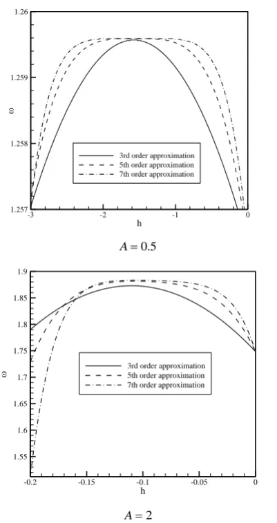
Finding a proper value for the auxiliary parameter, h, is crucial for accurate prediction of the response by the HAM. For this purpose,

the variation of the non-dimensional frequency,

, corresponding to the first two modes, are depicted in Figs. 2-3. Results are obtained for two different values of vibration amplitudes,

A. The best values of h correspond to the regions where the rate of change of  with h is zero. These values, however, are not the same for different amplitudes even when the seventh-order approximation is used. Similar results are also obtained for higher modes of vibration which confirms the necessity of using the homotopy-Pade technique for obtaining a unique expression for different vibration amplitudes.

h



-3 -2 -1 0

1.257 1.258 1.259 1.26

3rd order approximation 5th order approximation 7th order approximation

0.5

A

h



-0.2 -0.15 -0.1 -0.05 0 1.55

1.6 1.65 1.7 1.75 1.8 1.85 1.9

3rd order approximation 5th order approximation 7th order approximation

2

A

133 h



-2 -1.75 -1.5 -1.25 -1 -0.75 -0.5 -0.25 0

0.831 0.832 0.833 0.834 0.835 0.836 0.837 0.838 0.839 0.84 0.841 0.842 0.843 0.844 0.845 0.846

3rd order approximation 5th order approximation 7th order approximation

0.5

A

h



-0.075 -0.05 -0.025 0

0.4 0.5 0.6

3rd order approximation 5th order approximation 7th order approximation

2

A

Fig. 3. Variation of excitation frequency with auxiliary parameter h for the second mode.

Next, the accuracy of the analytical solution is examined in Figs. 4-7 by depicting the frequency-amplitude curves for the first four modes of vibration. Analytical results, based on the HAM, are obtained using the proper values of h for A2. The results of the [1, 1] homotopy-Pade technique and also the [2, 2] Pade approximant of the fifth order HAM solution are also included in these figures. It can be seen that the first order approximation is adequate for the first mode’s amplitudes smaller than 0.5. For higher modes, the nonlinearity seems to become stronger and thus the first order HAM is only accurate for A0.3. The third order approximation is also seen to

become closer to the numerical solution, even though that h is chosen based on the -h curve obtained for A2. Considering the close agreement of the third order HAM with the numerical result at A2, it may be expected that better result may have been obtained if h is separately determined for different values of A. However, this would considerably slow down the process of obtaining the whole frequency-amplitude curve. Instead, the homotopy-Pade technique is used here which is found to have a minimal dependence on h. In fact, the solution is found to be varied with h in a narrow region near h0. So taking an arbitrarily large value for h, say h 10, a unique expression can be obtained for all values of A. This is evident in Figs. 4-6, which shows excellent agreements between the [1, 1] homotopy-Pade and the numerical result, especially for the first and fourth modes. Slight discrepancy, however, exists for the second and third modes when

1.5

A , which has completely disappeared by using the [2, 2] homotopy-Pade technique. It must be mentioned here that the oscillation with

1

A is strongly nonlinear and the high accuracy of the solution obtained by the homotopy-Pade technique for this range of vibration amplitudes, completely confirm the significant power of the analytical method.



A

1.2 1.4 1.6 1.8

0 0.5 1 1.5 2

1st order HAM 3rd order HAM

[1,1] Pade (with 3rd order HAM) [2,2] Pade (with 5th order HAM) Numerical solution

134



A

0.7 0.8 0.9 1

0 0.5 1 1.5 2

1st order HAM 3rd order HAM

[1,1] Pade (with 3rd order HAM) [2,2] Pade (with 5th order HAM) Numerical solution

Fig. 5 . Frequency-Amplitude curve for the second mode (h 0.05 for the third order HAM).



A

0.4 0.5 0.6 0.7 0.8 0.9 1

0 0.5 1 1.5 2

1st order HAM 3rd order HAM

[1,1] Pade (with 3rd order HAM) [2,2] Pade (with 5th order HAM) Numerical solution

Fig. 6. Frequency-Amplitude curve for the third mode (h 0.03 for the third order HAM).



A

0.2 0.3 0.4 0.5 0.6 0.7 0.8 0.9 1 0

0.5 1 1.5 2

1st order HAM 3rd order HAM

[1,1] Pade (with 3rd order HAM) [2,2] Pade (with 5th order HAM) Numerical solution

Fig. 7. Frequency-Amplitude curve for the fourth mode (h 0.015 for the third order HAM).

5.Conclusions

The HAM and the homotopy-Pade technique were used to obtain an accurate and efficient analytical solution for the nonlinear vibration of a parametrically excited cantilever beam. An explicit expression was presented for the third order approximation of the amplitude-frequency of the system. It was found that proper values of the auxiliary parameter, h, change with the non-dimensional vibration amplitude, A, making the HAM not suitable for the rapid depiction of the frequency-amplitude curves. The homotopy-Pade technique was thus employed, which besides improving the convergence rate, gave the solution that was almost independent of the auxiliary parameter h. The numerical results were presented for different modes of vibration, using both the HAM and homotopy-Pade technique and compared with the numerical solution. Highly accurate results were obtained using the [1, 1] Pade approximant of the third order HAM for non-dimensional amplitudes smaller than 1.5. For larger amplitudes up to 2, the [2, 2] Pade approximant of the fifth order HAM was found to coincide with the numerical solution, showing the significant power of the method in solving oscillatory equations with the strong nonlinearity.

References

[1] M. N. Hamdan, A. A. Al-Qaisia, “B. O. Al-Bedoor, Comparison of analytical techniques for nonlinear vibrations of a parametrically excited cantilever”,

International Journal of Mechanical

Sciences, Vol. 43, No. 6, pp. 1521-1542,

(2001).

[2] E. C. Haight, W.W. King, “Stability of nonlinear oscillations of an elastic rod”,

Journal of the Acoustical Society of

America, Vol. 52, No. 3B, pp. 899-911,

(1971).

[3] R. S. Haxton, A. D. S. Barr, “The autoparametric vibration absorber”,

Transactions of the ASME, Journal of

Engineering for Industry, Vol. 94, No. 1,

135 [4] K. Sato, H. Saito, K. Otomi, “The

parametric response of a horizontal beam carrying a concentrated mass under gravity”, Transactions of the ASME

Journal of Applied Mechanics, Vol. 44,

No. 3, pp. 643-8, (1978).

[6] F.C. Moon, Experiments on chaotic motion of a forced nonlinear oscillator a strange attractors, Journal of Applied

Mechanics, Vol. 47, No. 3, pp. 639-44,

(1980).

[7] F. Pai, A.H. Nayfeh, “Nonlinear non-planar oscillations of a cantilever beam under lateral base excitations”, Journal of

Sound and Vibration, Vol. 25, No. 5, pp.

455-74, (1990).

[8] L. D. Zavodney, A. H. Nayfeh, “The nonlinear response of a slender beam carrying a lumped mass to a principal parametric excitation: theory and experiment”, International Journal of

Nonlinear Mechanics, Vol. 24, No. 2, pp.

105-25, (1989).

[9] T. D. Burton, M. Kolowith, “Nonlinear resonance and chaotic motion in a flexible parametrically excited beam”,

Proceedings of the Second Conference on Nonlinear Vibrations, Stability and

Dynamics of Structures and Mechanisms,

Blacksburg, VA, (1988).

[10] H. M. Sedighi, K. H. Shirazi and A. Noghrehabadi, “Application of recent powerful analytical approaches on the non-linear vibration of cantilever beams”,

International Journal of Nonlinear

Sciences and Numerical Simulation, Vol.

13, No. 7, pp. 487-494, (2012).

[11] H. M. Sedighi, K. H. Shirazi, “A new approach to analytical solution of cantilever beam vibration with nonlinear boundary condition”, Journal of

Computational and Nonlinear Dynamics,

Vol. 7, No. 3, pp. 1-4, (2012).

[12] H. M. Sedighi, K. H. Shirazi, A. Reza and J. Zare, “Accurate modeling of preload discontinuity in the analytical approach of the nonlinear free vibration of beams”, Proceedings of the Institution of Mechanical Engineers, Part C: Journal

of Mechanical Engineering Science, Vol.

226, No. 10, pp. 2474-2484, (2012). [13] H. M. Sedighi, K. H. Shirazi, M. A.

Attarzadeh, A study on the quantic nonlinear beam vibrations using asymptotic approximate approaches, Acta

Astronautica, Vol. 91, pp. 245-250,

(2013).

[14] H. M. Sedighi, A. Reza, “High precise analysis of lateral vibration of quintic nonlinear beam”, Latin American Journal of Solids and Structures, Vol. 10, No. 2, pp. 441- 452, (2013).

[15] H. M. Sedighi, F. Daneshmand, “Nonlinear transversely vibrating beams by the homotopy perturbation method with an auxiliary term”, Journal of Applied and Computational Mechanics, Vol. 1, No. 1, pp. 1-9 , (2015).

[16] S. J. Liao, Beyond Perturbation: Introduction to the Homotopy Analysis

Method, Chapman & Hall/CRC Press,

Boca Raton, (2003).

[17] S. J. Liao, K. F. Cheung, “Homotopy analysis of nonlinear progressive waves in deep water”, Journal of Engineering

Mathematics, Vol. 45, No. 2, pp.

105-116, (2003).

[18] S. J. Liao, A. Campo, Analytic solutions of the temperature distribution in Blasius viscous flow problems, Journal of Fluid

Mechanics. Vol. 453, No. 1, pp. 411-425,

(2002).

[19] T. Pirbodaghi, M. T. Ahmadian, M. Fesanghary, “On the homotopy analysis method for non-linear vibration of beams”, Mechanics Research

Communications, Vol. 36, No. 2, pp.

143-148, (2009).

[20] R. Wu, J. Wang, J. Du, Y. Hu, H. Hu, “Solutions of nonlinear thickness-shear vibrations of an infinite isotropic plate with the homotopy analysis method”,

Numerical Algorithms, Vol. 59, No. 2,

pp. 213-226, (2012).

136

homotopy”, Journal of solid mechanics, Vol. 6, No. 4, pp. 389-396, (2014). [22] H. M. Sedighi, K. H. Shirazi, J. Zare,

“An analytic solution of transversal oscillation of quintic non-linear beam with homotopy analysis method”,

International Journal of Non-Linear

Mechanics, Vol. 47, No. 7, pp. 777-784,

(2012).

[23] S. H. Hoseini, T. Pirbodaghi, M. T. Ahmadian, G.H. Farrahi, “On the large amplitude free vibrations of tapered beams: an analytical approach”,

Mechanic Research Communication,

Vol. 36, No. 8, pp. 892-897, (2009). [24] M. R. M. Crespo da Silva, C. C. Glynn,

“Nonlinear flexural-flexural-torsional dynamics of inextensible beams, I: equations of motion”, Journal of Structural Mechanics, Vol. 6, No. 4, pp. 437-48, (1978).

[25] A. H. Nayfeh, P. F. Pai, Linear and

Nonlinear Structural Mechanics, John

Wiley &Sons, Weinheim, (2004). [26] E. B. Saff, R. S. Varga, Pade and

Rational Approximation, Academic

Press, New York, (1977).

[27] J. Kallrath., On Rational Function Techniques and Pade Approximants. An

Overview, Report, Ludwigshafen,

Germany, (2002).

How to cite this paper:

S. Mahmoudkhani, “An efficient analytical solution for nonlinear

vibrations of a parametrically excited beam”, Journal of

Computational and Applied Research in Mechanical Engineering,

Vol. 7. No. 1, pp. 127-136

DOI:

10.22061/JCARME.2017.642