Tensor on tensor regression with tensor normal errors and tensor network states on the regression parameter

Creative Components Iowa State University Capstones, Theses and _{Dissertations}

Fall 2018

Tensor on tensor regression with tensor normal errors and tensor

Tensor on tensor regression with tensor normal errors and tensor

network states on the regression parameter

network states on the regression parameter

Carlos Llosa

Iowa State University, cllosa@iastate.edu

Follow this and additional works at: https://lib.dr.iastate.edu/creativecomponents

Part of the Multivariate Analysis Commons, Statistical Models Commons, and the Statistical Theory Commons

Recommended Citation Recommended Citation

Llosa, Carlos, "Tensor on tensor regression with tensor normal errors and tensor network states on the regression parameter" (2018). Creative Components. 82.

https://lib.dr.iastate.edu/creativecomponents/82

Tensor on Tensor Regression with Tensor Normal Errors and

Tensor Network States on the Regression Parameter

Carlos Llosa

Deparment of Statistics, Iowa State University

November 22, 2018

Abstract

With the growing interest in tensor regression models and decompositions, the ten-sor normal distribution offers a flexible and intuitive way to model multi-way data and error dependence. In this paper we formulate two regression models where the responses and covariates are both tensors of any number of dimensions and the errors follow a tensor normal distribution. The first model uses a CANDECOMP/PARAFAC (CP) structure and the second model uses a Tensor Chain (TC) structure, and in both cases we derive Maximum Likelihood Estimators (MLEs) and their asymptotic distri-butions. Furthermore we formulate a tensor on tensor regression model with a Tucker structure on the regression parameter and estimate the parameters using least squares. Aditionally, we find the fisher information matrix of the covariance parameters in an independent sample of tensor normally distributed variables with mean 0, and show that this fisher information also applies to the covariances in the multilinear tensor re-gression model [6] and tensor on tensor models with tensor normal errors regardless of the structure on the regression parameter.

1

Introduction

Multi-dimensional datasets are becoming more widely spread across multiple disciplines. Examples include multilinear relational data in political science and sociology and multi-dimensional imaging data in fields such as neurology and forestry. Multimulti-dimensional ar-rays have also been used in experimental design for treating n´factor crossed layouts, or multi-dimensional balanced split-plots [36]. Since the parameters neccesary to model multi-dimensional datasets using traditional statistical methods grows exponentially with the number of dimensions, the past decade has seen a growing interest in models that con-sider high dimensionality. The tensor GLM framework proposed in [42] and extended in [24] offers a way to regress a univariate response using tensor-valued predictors, and this task became known astensor regression. However, several other methods for the same task have been proposed, includying Bayesian Tensor Regression [14], Tensor Envelope Partial Least-Squares Regression [40], Hierarchical Tucker Tensor regression [19] and Support Ten-sor Machines [37]. Several other tensor regression frameworks have been proposed recently. See [23] and [34] for the task of regressing tensor valued responses using multivariate pre-dictors, [6] for the case when the covariates and predictors are tensors of the same number of dimensions, and [41] and [25] when the response and covariates are tensors of any dimen-sions.

The contributions of this paper are multiple. First, we provide tensor algebra notation and properties used in other disciplines such as physics and machine learning that can help with the development of multilinear statistics. Second, we review the tensor normal distribution, find new properties and generalize the MLE algorithm for maximum likelihood estimation [10]. Finally, we formulate two tensor on tensor regression models and derive their asymptotic distributions when the errors follow a tensor normal distribution, and one tensor on tensor model that uses least squares to the estimation of the parameters.

The rest of the paper is divided as follows. In section 2 we review tensor network diagrams, tensor algebra properties, the tensor normal distribution and linear regression models with normal errors. In section 3 we formulate tensor and study tensor on tensor regression models with tensor normal errors. In section 4 derive tensor on tensor regression with Tucker decomposition and Least Squares. Section 5 provides the asymptotics of all the models that follow the tensor normal distribution. Section 6 provides a simulation comparing one of our models with other already existing methods for regressing matrices on matrices. Finally, section 7 provides the proofs of all the theorems in the paper.

2

Preliminaries

Throghout this paper the trace is denoted using trp.q, the transpose usingp.q1, the determi-nant using |.|, the Moore–Penrose inverse usingp.q: and the identity matrix of sizenusing

In. The Kronecker product is denoted usingband the Khatri-Rao product is denoted using d. The vecp.q operator stacks the columns of a matrix into a vector and the commutation matrix Kk,lPRklˆkl matches the elements of vecpAq and vecpA1

q, see [26]

vecpA1q “Kk,lvecpAq, APRkˆl.

The half vectorization, denoted using vech, vectorizes the lower triangular side of a sym-metric matrix. The duplication matrix, denoted using Dk, is the full column rank matrix that matches the vectorization and half vectorization of a symmetric matrix

DkvechpAq “vecpAq, APRkˆk is symmetric.

The following matrix identities are useful for dealing with tensors

Properties 2.1. Suppose A1, . . . Ap are matrices of any size and Σ1, . . . ,Σp are square matrices of any size. Then

a. ˇˇ

1

 i“p

Σi| “ p ś i“1

|Σ i|m´i_{, m}

´i “ p ś

j“1 j‰i

rankpΣjq.

b. `

1

 i“p

Σi ˘´1

“`

1

 i“p

Σ´_i 1˘, `

1

 i“p

Ai ˘_|

“`

1

 i“p

A|_i˘ and `

1

 i“p

Ai ˘:

“`

1

 i“p

A:_i˘.

c. p Â

i“1

Ai “ `Âl

i“1

Aiq b` p Â

i“l`1

Aiq, l“1, . . . , p.

d. `

1

 i“p

Ai ˘`Â1

i“p

Bi ˘

“

1

 i“p

pAiBiq, whereBiare matrices such thatAiBi can be formed.

The following properties can be found in [27]. Suppose A1 PRmˆn and A2PRpˆq.

e. K1

m,n “Km,n´1 “Kn,m and Kn,mKm,n “Inm. f. Kp,mpA1bA2qKn,q“A2bA1,

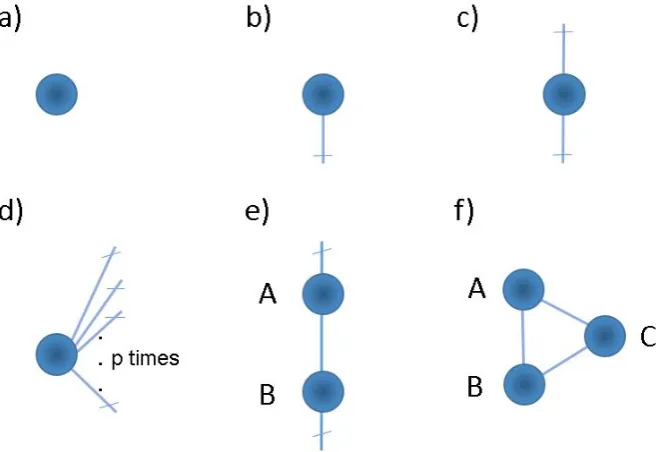
Figure 1: tensor network diagrams of a) a scalar, b) a vector, c) a matrix, d) a p´th dimensional tensor, e) the matrix product AB, and f ) the trace of the matrix product

ABC ptrpABCqq.

2.1 Tensor network diagrams

Tensor network diagrams are useful for visualizing tensor manipulations. They were orig-inally introduced in quantum physics to describe the hilbert space interactions that occur in many body problems (see [31]) and in high energy physics to represent invariants of quantum states (see [2]). They have been adapted to tensor models in machine learning in the past years (see [4] and [5]). These diagrams are critical in this paper because they allow us to identify tensor expressions that make estimation and formulation possible.

Each node corresponds to a tensor and the number of lines coming from the node represents a dimension, or mode. A node with no lines is a scalar, a node with one line is a vector, a node with two lines is a matrix and a node withplines is apthdimensional tensor (see Figure 1a-d). The contraction between two same-sized modes from (possibly) distinct tensors sums over all elements in the modes being contracted while leaving the other modes intact. For instance, the matrix product AB contracts the rows of A with the columns of

B, and the resulting columns and rows of AB result from the columns and rows of A and

B respectively (see Figure 1e). Contractions are represented in tensor network diagrams by merging the lines (modes) being contracted. A self contraction is a contraction between two lines coming from the same tensor, and is analogous to the trace (see Figure 1f).

2.2 Tensor notation and properties

Tensors are multidimensional arrays of numbers. The number of dimensions or indices of a tensor is called its order. Vectors are first order tensors and matrices are second order tensors. Following the notation in [4] we refer to scalars using lower case letters (ie. x), vectors using bold lower case italized letters (ie. xq, matrices using capital letters (ie. X) and higher order tensors using bold underlined capital letters (ie. X). The pi1, . . . , ipqth

element of a tensorXis denotedXpi1, . . . , ipq “xi1,...,ip. Similarly, subtensors are obtained

by fixing some of the indexes of the tensor. For instance mode´k fibers results from fixing all but the kth index of the tensor (ie: Xpi1,:, i3, i4qq, and slices result by fixing all but

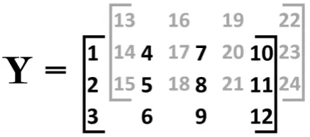
Figure 2: A third order tensor with elements 1 through 24

vector outer product (˝). For p“2 we havea1˝a2“a1a12, and for the general case

p ˝ j“1aj “

m1 ÿ

i1“1

. . .

mp ÿ

ip“1

”_źp

j“1

ajpijq ı _p

˝ j“1e

mj

ij , aj PR mj_{, j}

“1, . . . , p, (2.1)

where em_i PRm is a unit basis vector with 1 as theith element and 0 elsewhere.

Ap´th order tensorX has rank 1 if it can be written as the outer product ofpvectors. In general, the rank of a tensor is the minimum number of rank one tensors that add up to it. Since finding the rank of a higher order tensor is an NP-hard problem [20], most tensor manipulations choose the rank a priori based on the precision needed. Anypthorder tensor

XPRm1ˆ...ˆmp withpi1, . . . , ipqth elementxi1,...,ip can be expressed as

X“ m1 ÿ

i1“1

. . .

mp ÿ

ip“1

xi1...ip ` p

˝ q“1e

mq iq

˘

. (2.2)

Flattening or matricizing tensors allow us to use matrix algebra properties and effi-cient algorithms. The mode´kmatricization sets themode´k fibers as the columns of the resulting matrix

Xpkq“

m1 ÿ

i1“1

. . .

mp ÿ

ip“1

xi1...ipe mk ik

`â1 q“p q‰k

emq iq

˘1

. (2.3)

and the mode´k canonical matricization maps the first k modes to the rows and the rest of the modes to the columns of the resulting matrix

Xăką “

m1 ÿ

i1“1

. . .

mp ÿ

ip“1

xi1...ip `â1

q“k

em_iqq˘`

k`1

â

q“p

em_iqq˘1 (2.4)

Another useful reshaping is the vectorization, which stacks the mode´1 fibers

vecpXq “ m1 ÿ

i1“1

. . .

mp ÿ

ip“1

xi1...ip `

1

â

q“p

emq iq

˘

. (2.5)

Note that in equation (2.5) we defined tensor vectorization inreverse lexicographicorcolumn major order to avoid an incosistency with matrix vectorization. Column major order is the convention used in languages such as R and Matlab. Since this convention leads to multiple Kronecker products in reverse order, we can also use theleft Kronecker product (bL), which simply reverses the order of the Kronecker product (ie: BbA“AbLB).

As an example consider the third order tensor Y P R3ˆ4ˆ2 shown in figure 2. This

Mode 1 fibers Mode 2 fibers Mode 3 fibers » – 1 2 3 fi fl, » – 13 14 15 fi

fl, . . . , » – 22 23 24 fi fl » — — – 1 4 7 10 fi ffi ffi fl , » — — – 13 16 19 22 fi ffi ffi fl , . . . , » — — – 15 18 21 24 fi ffi ffi fl „ 1 13  , „ 4 16  , . . . , „ 12 24  .

Some of the slices ofY are

Yp:,:,1q “ »

–

1 4 7 10

2 5 8 11

3 6 9 12

fi

fl, Yp:,3,:q “ » – 7 19 8 20 9 21 fi

fl, Yp1,:,:q “ » — — – 1 13 4 16 7 19 10 22 fi ffi ffi fl

Themode-k matricizations are

X_p1q“ »

–

1 4 7 10 13 16 19 22

2 5 8 11 14 17 20 23

3 6 9 12 15 18 21 24

fi

fl, X_p2q“ »

— — –

1 2 3 13 14 15

4 5 6 16 17 18

7 8 9 19 20 21

10 11 12 22 23 24

fi

ffi ffi fl

,

X_p3q “ „

1 2 . . . 12

13 14 . . . 24



,

and themode-k canonical matricizations are

Yă1ą“Xp1q, Yă2ą “X1p3q, Yă3ą“vecpYq “

» — – 1 .. . 24 fi ffi fl.

The k´mode product (ˆk) between X PRm1ˆ...ˆmp and A P RJkˆmk _{multiplies every}

mode´kfiber ofXwithA, resulting inXˆkAPRm1ˆ...ˆmk´1ˆJkˆmk`1ˆ...ˆmpwith elements

`

XˆkA˘pi1, . . . , ipq “

mk ÿ

jk“1

xi1,...,ik´1,jk,ik`1,...,ipaik,jk. (2.6)

The k´th mode product applied to every mode is often called the Tucker product (see figure 3b) ([38] and [21] )

rrX;A1, . . . , Apss “Xˆ1A1ˆ2. . .ˆpAp“ m1 ÿ

i1“1

. . .

mp ÿ

ip“1

xi1...ip ` p

˝

q“1Aqp:, iqq

˘

. (2.7)

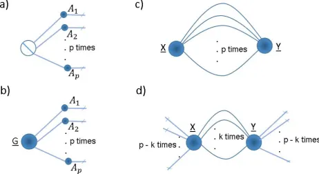
A diagonal tensor is a tensor with 0s everywhere but at the places where the indexes are all the same. They are represented in tensor network diagrams with nodes with a diagonal inside (see Figure 3a). If we let IPRRˆ...ˆR be a pth order diagonal tensor with 1s at the

diagonal and 0s elsewhere

I“ R ÿ

i“1

` p ˝ q“1e

R i

˘

, (2.8)

then the Tucker product applied to I with respect to Ai P RmiˆR for i “ 1, . . . , p can be expressed in canonical polyadic, or CANDECOMP/PARAFAC (CP) ([3], [17] and [21]) form (see figure 3a)

Figure 3: tensor network diagrams of a) the CP decomposition, b) the Tucker decomposi-tion, c) the inner product between two order p tensors of the same order and size, andd)

the partial´k contraction between two order p tensors with the same size along their first

k modes.

Note that as a result of equations (2.7), (2.8) and (2.9) the CP form can be expressed as

rrA1, . . . , Apss “

R ÿ

i“1

` p ˝

q“1Aqp:, iq

˘

, (2.10)

which means that the rank of rrA1, . . . , Apssis at most R. The tensor in equation (2.10) is

referred to as a Kruskal tensor. The following identities are important for the case when

p“2

X_p2q“X1_,

rrX;A1, A2ss “A1XA12, rrA1, A2ss “A1A12. (2.11)

Tensor decompositions allow us to decompose a tensor using lower order tensors. The CP decomposition decomposes a tensor in a series of rank one tensors (see figure 3a)

X“ R ÿ

r“1

p ˝p

j“1ajrq “ rrA1, . . . , Apss, Aj “ raj1. . .ajRs, (2.12)

and is often solved using an alternating least squares (ALS) algorithm where each step is obtained using property (2.1j) below. The Tucker decomposition decomposes thepth order tensor X into rrG;A1, . . . , Apss, where G is a smaller tensor of the same order as X and

A1, . . . , Ap are the factor matrices (see figure 3b). The Tucker decomposition is often solved in the form of the higher order singular value decomposition (HOSVD) [7] or hierarchical Tucker decomposition ([13] and [16]). One can also estimate the Tucker decomposition via ALS using theorems 2.1i and 2.1c below.

The inner product or contraction between two tensors of the same order and size is the sum of the product of their entries (see figure 3c)

xX,Yy “ m1 ÿ

i1“1

. . .

mp ÿ

ip“1

Figure 4: tensor network diagram of the Tensor Chain (TC) decomposition (also referred to as Matrix Product State (MPS) with periodic boundary conditions in physics) of a fifth order tensor Y.

This inner product is invariant under reshapings (see theorem 2.1g) and is used to define the Frobenius norm of a tensor

||X||F “axX,Xy. (2.14)

This definition of the Frobenius norm is consistent when p“2 andp“1 because

xX, Xy “trpXX1

q, xx,xy “x1_{x. (2.15)}

Tensors can also be contracted along individual modes. The mode-`k<sub>l</sub>˘ product or contrac-tion between X P Rm1ˆ...ˆmp and Y P Rn1ˆ...ˆnq, where ml “ nk, results in a tensor of order p`q´2 where the l´th mode of X gets contracted with thek´th mode of Y

Xˆm_n Y“ m1 ÿ

i1“1

. . .

ml´1 ÿ

il´1“1 ml`1

ÿ

il`1“1

. . .

mp ÿ

ip“1

n1 ÿ

j1“1

. . .

nk´1 ÿ

jk´1“1 nk`1

ÿ

jk`1“1

. . .

nq ÿ

jq“1

!_ÿml t“1

xi1,...,il´1,t,il`1,...,ipyj1,...,jk´1,t,jk`1,...,jq )

` p ˝ s“1 s‰l

ems is

˘ ˝` ˝q

s“1 s‰k

ens js

˘

. (2.16)

The same notation can be used to contract several modes between two tensors. The mode-`k1,...,ka

l1,...,la ˘

contraction between between X and Y where mk1 “ nl1, . . . , mka “ nla

results in a tensor of order p`q ´2ˆa where the modes indicated in the product get contracted. The partial´k contraction is a special case where the first k modes of X and

Y get contracted (See figure 3d)

xX,Yyk“Xˆ1₁,...,k_,...,kYPRmk`1ˆ...ˆmpˆnk`1ˆ...,nq. (2.17)

An important case of the partial contraction is when the first tensor has smaller order. For instance, if păq and mi “ni fori“1, . . . , pthen

xX|Yy “Xˆ1₁,...,p_,...,pYPRnp`1ˆ...,nq. (2.18)

Another special case is the contraction of the last mode ofXalong with the first mode of Y, denoted usingˆ1

Xˆ1Y“Xˆ1pY. (2.19)

The tensor trace can be seen as a self contraction between two outer modes; it has also been defined for multiple self-contractions. Suppose XPRRˆm1ˆ...ˆmpˆR, then

trpXq “ R ÿ

i“1

These last two definitions are useful for representing the Tensor Chain (TC) decomposition [32], or Matrix Product State (MPS) with periodic boundary conditions, as it is refered to in physics [31], which decomposes a p-th order tensorXPRm1ˆ...ˆmp intopdifferent third

order tensors Gpiq

PRgi´1ˆmiˆgi fori“1, . . . , pwhere g0 “gp`1 such that

X“trpGp1qˆ1. . .ˆ1Gppqq. (2.21)

See figure 4 for a tensor network diagram of the TC decomposition of a fifth order tensor. The following tensor algebra properties are critical in this paper. Theorem 2.1e can be found in [4] and theorems 2.1(i andj) can be found in [21].

Theorem 2.1. Suppose X,YPRm1ˆ...ˆmp. Then

a. vecpXq “ »

— –

vec`Xp:, . . . ,:,1, . . . ,1q˘

.. .

vec`Xp:, . . . ,:, mk`1, . . . , mpq

˘ fi

ffi

fl, k“1, . . . , p.

b. vec` ˝p i“1ai

˘ “

1

 i“p

ai, where a1, . . . ,ap are vectors of any size.

For p=2: vecpa1a12q “a2ba1

c. vecrrX;A1, . . . , Apss “

`Â1 i“p

Ai ˘

vecpXq, where AiPRniˆmi for anyni PN.

For p=2: vecpA1XA12q “ pA2bA1qvecpXq. d. vecpXq “vecpX_p1qq “vecpXăląq, l“1, . . . , p.

e. Xăp´1ą“X1_ppq

f. vecxX|By “B1

ăląvecX , XPR

m1ˆ...ˆml _{, lăp.}

g. xX,Yy “ pvecXq1pvecYq “ trpXpkqYp1kqq , where k “1, . . . , p and Y and X have

the same order and size.

h. xX,rrY; Σ1, . . . ,Σpssy “vecpXq1

`Â1 i“p

Σi ˘

vecpYq, ΣiPRmiˆmi_{, i“1, . . . , p.}

For p=2: trpXΣ2Y1Σ11q “ pvecXq1pΣ2bΣ1qpvecYq

i.

´

rrX;A1, . . . , Apss

¯

pkq “

AkXpkqA1´k, where A´k “

1

 i“j i‰k

Ai and Ai PRniˆmi for any

ni PN k“1, . . . , p.

j.

´

rrA1, . . . , Apss

¯

pkq “

Ak `Ä1

i“j i‰k

Ai ˘1

, k “ 1, . . . , p and A1, . . . , Ap have the same

number of columns.

k. vecpXpkqq “KpkqvecpXq, Kpkq“

`

Iśp

i“k`1mibKśk_i“1´1mi,mk ˘

.

2.3 The Tensor Normal Distribution and the Generalized MLE Algo-rithm

The multivariate normal distribution is perhaps the most important multivariate distribu-tion in statistics. The following results are well known and will be used to construct the tensor normal distribution. See [29] for more details.

Properties 2.2. Suppose the random vector xPRm is distributed according to the

mul-tivariate normal distribution with mean µ and positive definite covariance matrix Σ (ie: x„Nmpµ,Σq) then:

a. If A PRpˆm then Ax „NppAµ, AΣATq. Note that if AΣAT is not positive definite then the distribution is called singular multivariate normal.

b. The multivariate normalx has the probability density function

fpx;µ,Σq “ p2πq´m{2|Σ|´1{2exp

´ ´1

2px´µq T_Σ´1

px´µq ¯

c. If xiiid„ Nmpµi,Σq,i“1, . . . , n , then

»

— –

x1

.. . xn

fi

ffi

fl„Nnm ˜

»

— –

µ1

.. . µn

fi

ffi

fl, InbΣ ¸

.

The matrix normal distribution was studied extensively in the first chapter of [15]. To derive it consider the bivariate normal distribution

„

x1

x2

 „N2

´„_µ

1

µ2



,

„

σ₁₁2 σ2₁₂ σ₂₁2 σ2₂₂

 ¯

, (2.22)

where marginallyxi „Npµi, σii2qfori“1,2. Now think of the scalarsx1 andx2as the three

dimensional vectors that make up the columns of a matrix XPR3ˆ2. A slight modification

to equation (2.22) leads to the definition of the matrix normal distribution

vecpXq “ „

x1 x2



„N3ˆ2

´„_µ

1 µ2



,

„

σ2₁₁Σ1 σ122 Σ1

σ2₂₁Σ1 σ222 Σ1

 ¯

. (2.23)

Intuitively x1 and x2 can be thought of as observations from two multivariate normal distributions that share the same covariance matrix Σ1, and whose dependence is determined

by another covariance matrix Σ2ri, js “σ2ij.

Definition 2.1. A random matrixXPRm1ˆm2 follows a matrix normal distribution with

meanM PRm1ˆm2 _{and positive definite covariance matrices Σ}

1 PRm1ˆm1 _{and Σ}

2 PRm2ˆm2

(ie. X „Nm1,m2 `

M , Σ1,Σ2

˘

) if and only if vecpXq „Nm1ˆm2 `

vecpMq,Σ2bΣ1

˘

.

The tensor normal distribution was introduced in [1], [18], [28] and [30] as a general-ization of the matrix normal distribution to multiple dimensions. It is also referred to as the array variate normal distribution and the multilinear normal distribution. To derive it consider the random order three tensor XPR3ˆ2ˆ2 with marginally matrix normal frontal

slices Xp:,:, iq „ N3,2

`

Mi , σii3Σ1,Σ2

˘

for some constants σii, i “ 1,2. Then modifying equation (2.23) leads to the definition of the third order tensor normal distribution, also referred to as the trilinear normal distribution

vecpXq “ „

vecXp:,:,1q vecXp:,:,2q 

„N3ˆ2ˆ2

´„_vecM

1

vecM2



,

„

σ₁₁3 Σ2bΣ1 σ312Σ2bΣ1

σ₂₁3 Σ2bΣ1 σ322Σ2bΣ1

 ¯

Definition 2.2. A random tensor X P Rm1ˆ...ˆmp follows a pth order tensor normal

distribution with mean M P Rm1ˆ...ˆmp and positive definite mode covariance

matri-ces Σi P Rmiˆmi for i “ 1, . . . , p (ie. X „ Nm1,...,mp `

M ,Σ1, . . . ,Σp ˘

) if and only if vecpXq „Nm1ˆ...ˆmp

`

vecpMq,Â1

i“pΣi ˘

.

Note that not any multivariate normal vector can follow a tensor normal distribu-tion if shaped into a tensor, but only multivariate normal vectors with the required Kro-necker separable covariance structure. See [35] and [11] for tests on the assumption of Kronecker separability, which allows us to drastically reduce the number of free parame-ters required to estimate our covariance matrix. For instance consider the random ten-sor X P Rm1ˆ...ˆmp_{. If vecpXq follows a multivariate normal distribution then the}

co-variance matrix has “pśp_i“1mi `1qśp_i“1mi ‰

{2 free parameters. On the other hand if we let X „ Nm1,...,mp

`

M ,Σ1, . . . ,Σp ˘

, then the covariance matrix of vecpXq has only

řp

i“1pmi`1qmi{2 free parameters. The following results will be useful for tensor response

regression with tensor normal errors.

Algorithm 1: The generalized MLE algorithm for optimizing the complete log likelihood lpA1, . . . , Ap) using block descent

Input:Initial values Ap₂0q, . . . , App0q

1 k“0

2 whileconvergence criteria is not met do 3 Ap₁k`1q Parg max

A1

lpA1, Ap₂kq, . . . , Appkqq

4 Ap₂k`1q Parg max A2

lpAp₁k`1q, A2, Ap3kq, . . . ,Σ

pkq

p q.

5 ...

6 Appk`1q Parg max Ap

lpAp₁k`1q, . . . , A<sub>p</sub>pk<sub>´</sub>`₁1q, Apq

7 k“k`1

8 end

Theorem 2.2. Suppose X„Nm1,...,mp `

M ,Σ1, . . . ,Σp ˘

. Then a. rrX;A1, . . . , Apss „Nn1,...,npprrM;A1, . . . , Apss , A1Σ1A

1

1, . . . , ApΣpA1pq, Ai PRniˆmi_.

For p = 2: A1XA12 „Nn1,n2 `

A1M A12 , A1Σ1A11, A2Σ2A12q

˘

b. X_pkq „N_pmk,m

´kq ´

M_pkq , Σk,Σ´k ¯

, Σ´k“

1

Â

i“p i‰k

Σi, m´k“ p ś

i“1 i‰k

mi, k“1, . . . , p.

For p = k = 2: X1

„Nm2,m1 `

M1 _{, Σ}

2,Σ1

˘

c. X has the probability density function

fXpX;M,Σ1, . . . ,Σpq “

p2πq´ `_śp

i“1mi ˘

śp

i“1|Σi|´

m_´i 2 exp

´

´1₂xX´M,rrX´M ; Σ´1

1 , . . . ,Σ´p1ssy ¯

For p=2:

fXpX;M,Σ1,Σ2q “

p2πq´m1m2{2_|Σ

1|´m2{2|Σ2|´m1{2exp

´ ´1

2tr

“

Σ₁´1pX´MqΣ₂´1pX´Mq1‰ ¯

Figure 5: The trilinear tensor regression model

d. If X„Np,rp0,Σ1,Σ2q then EpXbXq “vecpΣ1qvecpΣ2q1. Proof. See appendix 7.2 for a proof.

Based on an iid sample from the tensor normal distribution, the maximum likelihood estimator (MLE) of the mean is the sample mean and the MLEs of the covariance matrices have no closed form solution but depend on each other. The MLE or flip-flop algorithm [10] uses a two-step block relaxation algorithm to estimate the covariance matrices in the matrix normal model. See theorem 5.1 for novel asymptotic results for these maximum likelihood estimators. We provide theMLE algorithm [10] as any algorithm that optimizes the complete likelihood using block relaxation where each block is the profile complete like-lihood (see algorithm 1). Other examples of block relaxation algorithms used in statistics include the expectation maximization (EM) algorithm and the alternating conditional ex-pectation (ACE) algorithm. See [8] for a review on block relaxation algorithms in statistics. Note that the algorithm might converge to a local maxima and this has to be dealt with in a case-by-case manner. In many cases initializing the algorithm with ?n´consistent estimators assure that the algorithm converges to estimators asymptotically equivalent to the MLE [22]. As a convergence criteria one can use the complete log likelihood or other criteria based on the change of parameters at each iteration. Examples ofMLE algorithms

in recent literature can be found in [6], [9], [12], [23] and [33].

2.4 Multivariate Linear Regressions and Multilinear Tensor Regression

The multivariate multiple linear regression model is critical to applications of the tensor normal distribution. We reformulate in the following way

Yi“AXi`Ei, Ei iid„ Np,r `

0,Σ, Ir ˘

, i“1, . . . , n. (2.25)

Here Yi is a response matrix with predictorXi PRqˆr and regression parameter APRpˆq.

The columns ofYi are independent from each other, and therefore this is equivalent to the more common formulation of multivariate multiple linear regression

Yip:, jq “AXip:, jq `eij, eij iid „ Np

`

0,Σ˘, i“1, . . . , n, j “1, . . . , r. (2.26)

Theorem 2.3. Suppose nr´q ěp. Then the MLEs of A and Σ are

ˆ

A“`

n ÿ

i“1

YiXi1 ˘`

n ÿ

i“1

XiXi1 ˘´1

, Σˆ “ 1

nr

n ÿ

i“1

pYi´AXˆ iqpYi´AXˆ iq1.

Proof. See appendix 7.3.1.

Another multivariate regression problem that is critical to this paper is

yi“Xiβ`ei, ei iid„ Np `

Figure 6: tensor network diagram of the multilinear tensor regression model

Here yi P Rp is a response vector with predictor matrix Xi P Rpˆq and regression

parameterβPRq. This is not a regular multivariate linear regression model and is analogous

to generalized least squares regression, therefore we refer to it as generalized multivariate regression. For our purposes we will only concentrate in the estimation of β.

Theorem 2.4. Suppose npěq. Then given Σ the MLE of β is

ˆ β“`

n ÿ

i“1

X_i1Σ´1Xi ˘´1`

n ÿ

i“1

X_i1Σ´1yi ˘

.

Proof. See appendix 7.3.2.

Multilinear tensor regression is a model where the responses and predictors are tensors of the same order. It works by fitting a separate multivariate linear regression on each side of the tensor and iterating the regression parameters until convergence using a generalized MLE algorithm. It was proposed by P. Hoff in [6], where he also proposed a Bayesian approach to the estimation of the parameters. Figure 5 shows the trilinear tensor regression model and figure 6 shows a tensor network diagram of the general model, which can be expressed as

Y_i“ rrX_i;M1, . . . , Mpss `Ei, Ei iid

„Nm1,...,mpp0 ; Σ1, . . . ,Σpq, i“1, . . . , n. (2.28)

Here Y_i P Rm1ˆ...ˆmp is the tensor response, Xi P Rh1ˆ...ˆhp its corresponding tensor covariate and E_i the tensor normal noise. The regression parameters or matrix factors are

Mj PRmjˆhj for i“1, . . . , p. To estimate Mk and Σk with all the other parameters fixed first apply the k´mode matricization to both sides of equation (2.28) using theorems (2.1i) and (2.2b)

Yipkq “MkXipkqM´1k`Ei, Eiiid„Nmk,m´kp0 ; Σk,Σ´kq, k“1, . . . , p. (2.29)

Note that this has a bilinear tensor regression form itself, where the covariates and responses are both matrices. However the purpose of equation (2.29) is only to find steps in the MLE algorithm forMkand Σk givenM´k and Σ´k. Using property (2.2a) we can write equation (2.29) as

YipkqΣ ´1{2

´k “MkXipkqM´1kΣ

´1{2

´k `Ei, Ei iid

„ Nmk,m´kp0 ; Σk, Im´kq, k“1, . . . , p,

(2.30) which is a multivariate multiple regression model with MLEs given in theorem 2.3:

ˆ

Mk“

n ÿ

i“1

YipkqΣ´´k1M´kXi1_pkq

”_ÿn

i“1

XipkqM´1kΣ´´1kM´kXi1_pkq

ı´1

Figure 7: tensor network diagram of the tensor on tensor model

and

ˆ Σk“

1

nm´k n ÿ

i“1

pYipkq´MkXipkqM 1

´kqΣ´´1kpYipkq´MkXipkqM 1

´kq1. (2.32)

See theorem 5.3 for novel asymptotic results of the general model. The bilinear tensor regression model is commonly refered to as matrix variate regression. It was coined by C. Viroli in [39] but fully estimated by Hoff in [6] and Ding and Cook in [9]. Ding and Cook also proposed envelope models for the matrix variate regression model, which can be extended to the multilinear tensor regression model.

2.5 Tensor on Tensor Regression

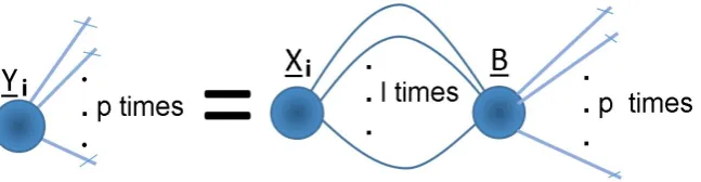
Tensor on tensor regression works by estimating a tensor with the combined order of the tensor response and covariate. See Figure 7 for a tensor network diagram of the model, which can be expressed as

Y_i “ xX_i|By, i“1, . . . , n. (2.33)

Here Y_i P Rm1ˆ...ˆmp is the tensor response, Xi P Rh1ˆ...ˆhl its corresponding tensor covariate and B P Rh1ˆ...ˆhlˆm1ˆ...ˆmp _{is the regression parameter. This form was first}

proposed in [25], which constrained B to have CP structure and solved the regression problem using least squares and ridge regularization. Vectorizing both sides of equation (2.33) and using theorem (2.1f) we obtain

vecpY_iq “B1

ăląvecpXiq, i“1, . . . , n, (2.34)

which is a multivariate regression problem and therefore the least squares solution is the same as the maximum likelihood estimator under normal errors given in theorem 2.3

ˆ

Bălą“

´_ÿn

i“1

pvecX_iqpvecX_iq1

¯´1´_ÿn i“1

pvecX_iqpvecY_iq1 ¯

. (2.35)

However solving for B_OLS often leads to overparameterization because of its size, which is

śp

i“1miˆ śl

i“1hi.

The rest of this paper will model the errors in equation (2.33) with the tensor normal distribution and impose different tensor structures onBto reduce its number of parameters. I will find MLEs of the tensor factors and covariance matrices and find asymptotic results.

3

Tensor on Tensor Regression with Tensor Normally

Dis-tributed Errors

Tensor on tensor regression can also be formulated using the tensor normal distribution

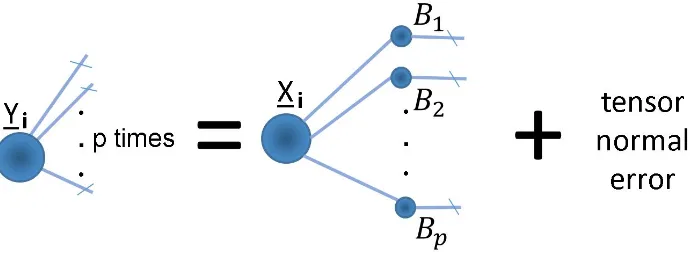
Y_i“M` xX<sub>i</sub>|By `E_i, E_iiid„Nm1,...,mpp0 , Σ1, . . . ,Σpq, i“1, . . . , n. (3.1)

This model offers a flexible way to model the covariance structure in our data. For instance, one could impose Σ1 to have an AR structure, and thus generalize vector

Figure 8: tensor network diagram of the tensor on tensor regression model where the re-gression parameter is constrained to a CP form

Figure 9: tensor network diagram that is equivalent to figure 8

The intercept term in equation 3.1 can be found by first fitting the model on centered covariates and responses, and finding Mˆ “ Y¯ ´ xX¯|By afterwards, where Y¯ and X¯ are the mean response and covariate respectively. In this section we will present two novel tensor on tensor regression models based on equation (3.1) that differ on the structure of

B. The first one imposes a CP structure and the second one imposes a TC structure, which has been shown to be effective in high dimensional problems. In both cases we will find maximum likelihood estimators for the tensor factors that depend on each other, and therefore we will optimize the likelihood using an MLE algorithm. Additionally the MLE algorithm will be used to find initial values for Σ1 . . . ,Σpas in [28], which have been shown to be ?n´consistent estimators in [23]. This way we make sure the MLE algorithm finds estimators that are asymptotically equivalent to the maximum likelihood estimators. As a convergence criteria we can use the change in likelihood at each step; however the estimators for the covariances are already close to the maxima, and therefore we will use the change in Frobenius norm of B instead.

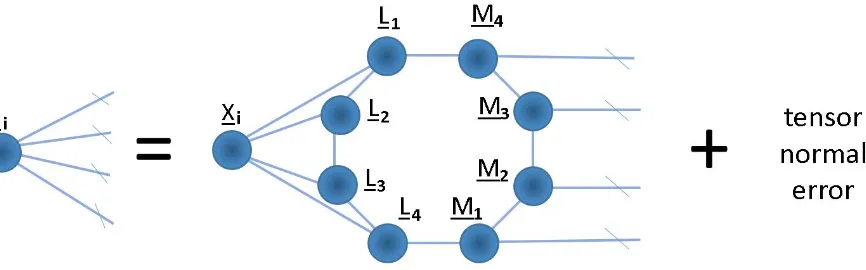
3.1 Tensor on Tensor Regression with CP structure on the Regression Parameter

Consider model (3.1) where the regression parameter has the CP structure

B“ rrL1, . . . , Ll, M1, . . . , Mpss. (3.2)

Here all the factor matrices haveRrows, meaning that the rank ofBis constrained to be at mostR. This way the number of free parameters inBare reduced from śl

i“1hiˆ śp

i“1mi to Rˆ přl_i“1hi `

řp

i“1miq. Note that by assuming that all the covariance matrices are

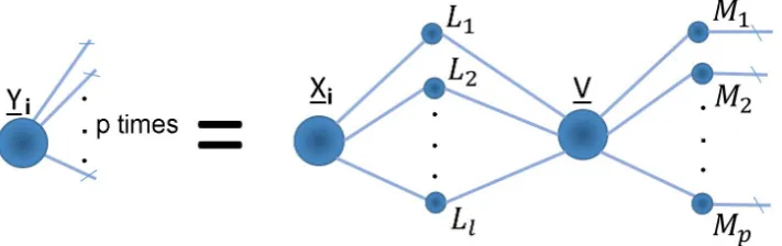
identity matrices, we generalize the model in [25], who solved the same regression model using least squares. See figure 8 for a tensor network diagram of this model. To estimate

M1, . . . , Mp and Σ1, . . . ,Σp first let

where IPRRˆ...ˆR is a diagonal tensor as in equation (2.8) and therefore Gi is a diagonal tensor too. Now we can write equation (3.1) as

Y_i “ rrG_i;M1, . . . , Mpss `Ei, Ei iid

„ Nm1,...,mpp0 , Σ1, . . . ,Σpq, i“1, . . . , n. (3.4)

Equation (3.4) is a multilinear tensor regression as in equation (2.28) with MLEs given in equations (2.31) and (2.31):

ˆ

Mk“

n ÿ

i“1

Yipkq

´_â1 i“p i‰k

Σ´_i 1Mi ¯

Gi1_pkq ”ÿn

i“1

Gipkq

´_â1 i“p i‰k

M_i1Σ´_i1Mi ¯

Gi1_pkq ı´1

(3.5)

and

ˆ Σk “

1

nm´k n ÿ

i“1

´

Yipkq´MkGipkq

1

â

i“p i‰k

M1

i ¯_â1

i“p i‰k

Σ´1

i ´

Yipkq´MkGipkq

1

â

i“p i‰k

M1

i ¯1

. (3.6)

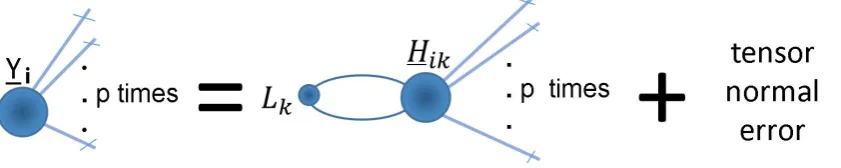
To find the maximum likelihood estimator of Lk fork“1, . . . , l first let

H_ik “X_iˆ1_1,...,k,...,k´_´1_1,k,k`<sub>`</sub>1_1,...,l,...,lrrL1, . . . , Lk´1, IR, Lk`1, . . . , Ll, M1, . . . , Mpss. (3.7)

The role H_ik plays in the estimation ofLk can be seen in figure 9. Both the rows and columns ofLkare contracted to eachHikand therefore we can only identify its vectorization. Vectorizing both sides of equation (3.1) with the constraint in (3.2) results in

vecpY_iq “Hik1ă2ąvecpLkq `ei, ei

iid

„Nm1ˆ...ˆmp ´

0 ,

1

â

i“p Σi

¯

, i“1, . . . , n. (3.8)

Note that equation (3.8) is a generalized multivariate regression as in equation (2.27) and therefore the MLE of vecpLlq is given in theorem 2.4 as

{

vecpLkq “ ´_ÿn

i“1

Hikă2ą

`

1

â

i“p Σi

˘´1

Hik1ă2ą

¯´1´_ÿn i“1

Hikă2ą

`

1

â

i“p Σi

˘´1

vecpY_iq ¯

. (3.9)

As in the usual CP decomposition, the columns of the factor matricesM1, . . . , Mp,L1, . . . , Lp are normalized for identifiability and stability purposes and the column norms of the last factor matrix is stored separately. See theorem 5.4 for asymptic results of our maximum likelihood estimators.

3.2 Tensor on Tensor Regression with TC structure on the Regression Parameter

Now consider model (3.1) where the regression parameter has the TC structure

B“trpLp1qˆ1. . .ˆ1Lplqˆ1Mp1qˆ1. . .ˆ1Mppqq. (3.10)

Here Lpiq P Rgi´1ˆhiˆgi _{for i“ 1, . . . , l and M}piq _{P R}gi`l´1ˆmiˆgi`l _{and i “ 1, . . . , p where}

g0 “ gp`l. By imposing a TC structure on B we reduce its number of free parameters from śl

i“1hiˆ śp

i“1mi to řl

i“1gi´1higi` řp

i“1gi`l´1migi`l. This formulation offers the advantage that not all the factor matrices need to have the same number of columns, which is useful when the size of the modes in our response or covariates are radically different, as in color images. This is phenomena is reffered to as skewness in modality. Note also that the TC decomposition has been shown to be effective in large dimensions. See figure 10 for a tensor network diagram of the regression model. To estimateMpkq_{and Σ}

Figure 10: tensor network diagram of the tensor on tensor regression model with TC struc-ture on the regression parameter.

Figure 11: tensor network diagram equivalent to figure 10.

Z_ik“Mpk`1qˆ1. . .ˆ1Mppqˆ1Riˆ1Mp1qˆ1. . .ˆ1Mpk´1q (3.11) where Ri PRg0ˆgl _{is the matrix}

Ri “ ´

Lp1qˆ1. . .ˆ1Lplq

¯

ˆ1₂,...,l_,...,l`1X_i. (3.12)

The role that Z_ik plays in the estimation of Mpkq _{can be seen in figure 11. Note that}

Z_ik P Rgk`lˆmk`1ˆ...ˆmpˆm1ˆ...ˆmk´1ˆgk`l´1_{. Let Z}˚

ik be its reshaping such that Z˚ik P Rgk`l´1ˆgk`lˆm1ˆ...ˆmk´1ˆmk`1ˆ...ˆmp_{, such a reshaping can be done with the functionaperm}

in base R. Applying the k-th mode matricization to both sides of equation (3.1) leads to

Yipkq “M pkq p2qZ

˚

ikă2ą`Ei, Ei

iid

„ Nmk,m´kp0 ; Σk,Σ´kq, i“1, . . . , n. (3.13)

which is on the bilinear tensor regression form as in equation (2.29) and with MLEs given in equations (2.31) and (2.32)

Mp_pk₂q_q “ n ÿ

i“1

YipkqΣ´

1

´kZ

˚

ik1ă2ą

”_ÿn

i“1

Z˚

ikă2ąΣ ´1

´kZ

˚

ik1ă2ą

ı´1

(3.14)

and

ˆ Σk“

1

nm´k n ÿ

i“1

pYipkq´M pkq p2qZ

˚

ikă2ąqΣ ´1

´kpYipkq´M pkq p2qZ

˚

ikă2ąq

1_{. (3.15)}

To estimateLpkq _fork

“1, . . . , l first let

N_ik “X_iˆl₁`<sub>,...,k</sub>p`2_´´₁k,...,l<sub>,k`1,...,l</sub>`p,2,...,l´k`1Jpkq (3.16) where Jpkq is the MPS tensor withoutLpkq

Figure 12: tensor network diagram equivalent to figure 10.

Figure 13: tensor network diagram of the tensor on tensor regression model where the regression parameter is constrained to a Tucker form

The role that N_ik plays in the estimation ofLpkq _{can be seen in figure 12. Note that N}

ik P Rhkˆgkˆm1ˆ...ˆmpˆgk´1_{. Let N}˚

ik be its reshaping such that N˚ik PRgk´1ˆhkˆgkˆm1ˆ...ˆmp. Then vectorizing both sides of equation (3.1) leads to

vecpY_iq “N˚

ik

1

ă3ąvecpL pkq

q `ei, ei

iid

„Nm1ˆ...ˆmp ´

0 ,

1

â

i“p Σi

¯

, i“1, . . . , n. (3.18)

Note that equation (3.18) is a generalized multivariate regression as in equation (2.27) and therefore the MLE of vecpLlq is given in theorem 2.4 as

{

vecpLpkq

q “ ´_ÿn

i“1

N˚

ikă3ą

`

1

â

i“p Σi

˘´1

N˚

ik

1 ă3ą

¯´1´_ÿn i“1

N˚

ikă3ą

`

1

â

i“p Σi

˘´1

vecpY_iq ¯

. (3.19)

See theorem 5.5 for asymptotic results of the regression parameters.

4

Tensor on Tensor Regression Using Least Squares

Note that all the methods found using MLE can be solved using LS by assuming that the covariance matrices are identity. In the case where the regression parameter is constrained to a CP form then this is equivalent to [25]. However some useful tensor structures are not estimable via MLE, and that includes the case where the regression parameter is constrained to a Tucker form. In this section we will solve this regression model using least squares.

4.1 Tensor on Tensor using The Tucker decomposition

Since the CP decomposition is a special case of the Tucker decomposition, in this section we will generalize the model proposed in [25] using the Tucker decomposition. In the context of tensor regression, this generalization is analogous to how [24] generalized [42]. This formulation is useful when data is skewed in modality. Consider the model in equation (2.33) where B now has the Tucker form

See figure 13 for a tensor network diagram of the model. To estimate M1, . . . , Mp first let

G_i“ xX_i,Vˆ1L1ˆ2. . .ˆlLlyl, i“1, . . . , n, (4.2)

Then fork“1, . . . , pthe LS estimators ofMk is given in equation (3.6) where Σl“Iml for

l“1, . . . , p.To find the estimator of Lk first let

H_ik “X_iˆ1₁,...,k_,...,k´_´1₁,k<sub>,k`</sub>`₁1,...,l_,...,lrrV;L1, . . . , Lk´1, IR, Lk`1, . . . , Ll, M1, . . . , Mpss. (4.3) Then the LS estimator of Lk is found in equation (3.9) where Σl“Iml for l“1, . . . , p. To

estimate V we first vectorize equation (2.33) using equation (2.1f)

vecpY_iq “`

1

â

i“p

Mi ˘

V1_ălą`

1

â

i“l

L1_i˘vecpX_iq, i“1, . . . , n. (4.4)

Then because of property (2.1b) and theorem (2.1c) the OLS estimator of V in equation (4.4) is the same as in

vecrrY_i;M₁:, . . . , M_p:ss “V1_ăląvecrrX_i;L1₁, . . . , L1_lss, i“1, . . . , n. (4.5) Therefore the OLS estimator of V is

p

Vălą“

»

— –

pvecrrX₁;L1

1, . . . , L1lssq1 ..

. pvecrrX_n;L1

1, . . . , L1lssq1 fi

ffi fl

:»

— –

pvecrrY₁;M₁:, . . . , Mp:ssq1 ..

.

pvecrrY_n;M₁:, . . . , Mp:ssq1 fi

ffi

fl. (4.6)

The estimators are found iteratively using an ALS algorithm until the Frobenius norm of

Bis smaller than a certain threshold. One can also constraint the columns ofL1, . . . , Ll, M1, . . . , Mp to have unit norm for identifiability and numerical stability.

5

Asymptotics

In this section we derive asymptotic results that apply to our models but also generalize to other models. First we find the fisher information matrix that corresponds to the covariance matrices under tensor normality with mean 0 (theorem 5.1) and show that they are the same as in tensor on tensor regression when the errors are assumed to be tensor normal (theorem 5.2). We proceed showing asymptotic independence between the MLE of the regression parameter and the covariance matrices (theorem 5.2), which is analogous to the multivariate case. This result allows us to focus on the regression parameter independently from the covariances. We next find the asymptotic variance of the parameters in the multilinear tensor regression model [6] (theorem 5.3) and finally we find the asymptotic variance of the parameters in the tensor on tensor regression model under normality when the repression parameter is assumed to have a CP form (theorem 5.4) and a TC form (theorem 5.5).

The following theorem finds the asymptotic variance of the MLEs of the covariance matrices under tensor normality with mean 0 [28]. This results applies also to the matrix normal case in the original MLE algorithm [10].

Theorem 5.1. Suppose X₁, . . . ,X_niid„Nm1,...,mp `

0 ,Σ1, . . . ,Σp ˘

.

Let θΣ “ rpvech Σ1q1, . . . ,pvech Σpq1s1, then the Fisher information matrix IΣ is a block matrix with kth block diagonal matrix (k“1, . . . , p)

E ´

´ B

2_lpΣkq

Bpvech ΣkqBpvech Σkq1 ¯

“ nm´k

2 D

1

mkpΣ

´1

k bΣ

´1

k qDmk

and pk, lqth off-diagonal block matrix where k, l“1, . . . , p, k‰l, m´kl“ śp

i“1,i‰k,i‰lmi,

E ´

´ B

2_lpΣ

k,Σlq Bpvech ΣkqBpvech Σlq1

¯

“ nm´kl

2 D

1

mk `

Proof. See appendix 7.4.1.

The next theorem shows that the asymptotic variance of the unstructured regression parameter is independent from the asymptotic variance of the MLEs of the covariance matrices. This result is important because we already found the asymptotic variance of the covariance matrices in theorem 5.1 and therefore it allows us to focus only in the asymptotic variance of the regression parameter, regardless of its structure.

Theorem 5.2. For i“1, . . . , n suppose that Y_i iid„Nm1,...,mp `

xX_i|By ,Σ1, . . . ,Σp ˘

. If θ “ rvecpB1

ăląq 1_θ1

Σs1, where θΣ “ rpvech Σ1q1, . . . ,pvech Σpq1s1, then the asymptotic vari-ance of θ is

avarpθq “ »

– ´ n

ř i“1

pvecX_iqpvecX_iq1 ¯´1

b ´ 1

 i“p

Σi ¯

0

0 I´Σ1

fi

fl

where IΣ is given in theorem 5.1. Proof. See appendix 7.4.2.

Now we will use the previous two theorems to find the asymptotic variance of the multilinear tensor regression model [6] under tensor normal errors. This proof also applies to any type of tensor on tensor regression that uses theorem 2.3 to obtain the MLEs of the tensor factors and will be used in the proof of theorems 5.4 and 5.5. This result generalizes the asymptotic findings for matrix variate regression in [9].

Theorem 5.3. Fori“1, . . . , n suppose thatY_i iid„Nm1,...,mp `

rrX_i;M1, . . . , Mpss ,Σ1, . . . ,Σp ˘

. Let θM “ rvecpM1q1. . .vecpMpq1θ_Σ1 s1 where θΣ “ rpvech Σ1q1, . . . ,pvech Σpq1s1. Then the asymptotic variance of θM is

avarpθMq “ » — — — — — — — — — — — — –

S´1

21 bΣ1 P1

´

Inb `Â1

i“p Σi

˘¯

P1

2 . . . P1

´

Inb `Â1

i“p Σi ˘¯ P1 m 0 P2 ´

Inb `Â1

i“p Σi

˘¯

P1

1 S22´1bΣ2 . . . P2

´

Inb `Â1

i“p Σi ˘¯ P1 m 0 .. . ... . .. ... ... Pm ´

Inb `Â1

i“p Σi

˘¯

P1

1 Pm ´

Inb `Â1

i“p Σi

˘¯

P1

2 . . . S2´m1bΣp 0

0 0 . . . 0 I´Σ1

fi ffi ffi ffi ffi ffi ffi ffi ffi ffi ffi ffi ffi fl

where S2k“ n ř i“1

Xipkq

´ 1 Â

i“p i‰k

M1

iΣ´

1

i Mi ¯

Xi1pkq, Pk “ pQ 1

kbImkqpInbKpkqq,

Qk “ » — — — — — — — — – ´ 1 Â

i“p i‰k

Σ´_i 1Mi ¯

Xi1pkqS ´1 2k .. . ´ 1 Â

i“p i‰k

Σ´_i 1Mi ¯

Xi1pkqS ´1 2k fi ffi ffi ffi ffi ffi ffi ffi ffi fl

, and Kpkq is given in theorem 2.1k.

Proof. See appendix 7.4.3.

parameter when the errors are assumed to be tensor normal, as in section 3.1. We use theorem 5.3 for the asymptotic variance of M1, . . . , Mp because they were found using theorem 2.3. Further, the asymptotic variance of L1, . . . , Lp can be used whenever the MLEs of the matrix factors are obtained using theorem 2.4 and will be used in the proof of theorem 5.5.

Theorem 5.4. For i“1, . . . , n suppose that Y_iiid„Nm1,...,mp `

xX_i|By ,Σ1, . . . ,Σp ˘

. Fur-thermore letB“ rrL1, . . . , Ll, M1, . . . , MpssandθCP “ rvecpL1q1. . .vecpLlq1vecpM1q1. . .vecpMpq1s1 , then the asymptotic variance of θCP is

avarpθCPq “ „

L J

J1 _M

 where L“ » — — — — — — — — — — –

S₁₁´1 R1

´

Inb `Â1

i“p Σi

˘¯

R1

2 . . . R1

´

Inb `Â1

i“p Σi ˘¯ R1 l R2 ´

Inb `Â1

i“p Σi

˘¯

R1

1 S

´1

12 . . . R2

´

Inb `Â1

i“p Σi ˘¯ R1 l .. . ... . .. ... Rl ´

Inb `Â1

i“p Σi

˘¯

R1

1 Rl ´

Inb `Â1

i“p Σi

˘¯

R1

2 . . . S1´l1

fi ffi ffi ffi ffi ffi ffi ffi ffi ffi ffi fl , J “ » — — — — — — – R1 ´

Inb `Â1

i“p Σi

˘¯

P1

1 . . . R1

´

Inb `Â1

i“p Σi ˘¯ P1 m .. . . .. ... Rl ´

Inb `Â1

i“p Σi

˘¯

P1

1 . . . Rl ´

Inb `Â1

i“p Σi ˘¯ P1 m fi ffi ffi ffi ffi ffi ffi fl ,

S1k“ n ř i“1

Hikă2ą

`Â1 i“p

Σi ˘´1

Hik1ă2ą, Rk“ rS ´1

1kH1kă2ą

`Â1 i“p

Σi ˘´1

. . . S₁´_k1Hnkă2ą

`Â1 i“p

Σi ˘´1

s,

Hik are given in equation (3.7) and M “avarpθMq is given in theorem 5.3 with S2k and

Qk given in theorem 5.3 by replacing Gi (given in equation 3.3) withXi.

Proof. See appendix 7.4.4.

Note that the asymptotic variance of each vecLk does not have a Kronecker separable structure and thus they dont follow asymptotically a matrix normal distribution. The following theorem uses all of our previous results.

Theorem 5.5. For i“1, . . . , n suppose that Y_iiid„Nm1,...,mp `

xX_i|By ,Σ1, . . . ,Σp ˘

. Fur-thermore let B“trpLp1q

ˆ1. . .ˆ1Lplq

ˆ1Mp1q

ˆ1. . .ˆ1Mppq

q and

θT C “ rvecpLp1qq1. . .vecpLplqq1vecpM_pp1₂q_qq1. . .vecpM_ppp₂q_qq1s1, then the asymptotic variance of

θT C is

avarpθT Cq “ „

L J

J1 _M



,

where LandJ are given in theorem 5.4 with S1k andRk obtained by replacingHikă2ą with

N˚

ikă3ą (given in equation 3.16) and M “avarpθMq is given in theorem 5.3 with

S2k“ řn

i“1Z˚ikă2ąΣ ´1

´kZ˚ik1ă2ą and Qk“

» — — — — — — — — – ´ 1 Â

i“p i‰k

Σ´1

i ¯

Z˚

ik1ă2ąS ´1 2k .. . ´ 1 Â

i“p i‰k

Σ´_i1

¯

Z˚

ik

1 ă2ąS

Proof. See appendix 7.4.5.

6

Simmulation

In this section we will compare four methods for regressing matrices on matrices. The first method is tensor on tensor regression using least squares [25], which we refer to as LSCP. The second method is tensor on tensor regression using maximum likelihood estimation, as in section 3.1, which we refer to as MLECP. The third method is matrix variate re-gression [9] (we use their implementation) or bilinear tensor rere-gression [6], which we refer to as MATREG. The last method is matrix variate regression with envelope models [9], which we refer to as MATREGENV; we used stepwise BIC to select the envelope size, as implementated in the paper.

Our covariates Xi and responses Yi are both 10ˆ10 matrices. The ith covariate is composed elementwise from simulations of the normal distributions with mean 100i and variance 10. The regression parameter BPR10ˆ10ˆ10ˆ10 is a tensor composed elementwise

from simulations of the gamma distribution with parameters α “200, β “1. The covari-ance matrices are both quadratic forms of matrices composed of normal distributions with variance 1 and means 4 and 1 corresponding to the first and second covariance matrix.

Note that in this simulation both MATREG and MLECP have the same number of paramaters because we restricted the CP rank of the regression parameters toR“5. In this case MATREG has two 10ˆ10 regression parameters and MLECP has four 5ˆ10 regression parameters, and both have the same number of parameters in the covariance structure. LSCP has a smaller number of parameters because it lacks a covariance structure and MATREGENV also has a smaller number of parameters because of the sparcity constraint. We simulatedn“1500 pairs of datapXi, Yiqand implemented the methods using seven different sample sizes : n “100,200,300,500,800,1000 and 1500. For comparison we use the Mean Sum of Standardized Squared Errors (MSSSE) criteria defined as

M SSSE“ 1

n

n ÿ

i“1

||Σp

´1{2

1 pYi´Y

est i qΣp

´1{2 2 ||

2

F, Yiest “Mx` xXi|Bpy

and assume that the LS methods have both covariances set to identity. This MSSSE criteria is analogous to the univariate case _n1řn

i“1pyi´yiestq{σˆ where the estimation of ˆσ is useful for assesing the predictive error.

Figure 14 shows a comparison between MSSSE among all methods. We can observe that the least squares method performs the worst because it did not account for the variability in the data. All the other methods perform well in the presence of heteroskedastic errors

Figure 15 shows a comparison between matrix variate regressions and MLECP. We can observe that MLECP outperforms the matrix variate regression even though they have the same number of parameters. This is perhaps the data was generated from a structure similar to MLECP.

Figure 15: Comparison of MSSSE among all methods except LSCP

Finally Figure 16 shows MLECP alone. We can observe that the MSSSE decays rapidly as the sample size increases.

7

Appendix

7.1 Proof of theorem 2.1: tensor algebra properties

Proof. For the following proofs note that the matrix product between A P Rm1ˆm with

elements Api, jq “aij and BPRmˆm2 with elementsBpi, jq “bij can be expressed as

AB“

m1 ÿ

i1“1 m ÿ

j“1

”

ai1jpe m1 i1 qpe

m j q1

ı_ÿm

j“1

m2 ÿ

i2“1 ”

bji2pe m j qpemi22q

1ı

“ m1 ÿ

i1“1

m2 ÿ

i2“1

”_ÿm

j“1

ai1jbji2pe m1 i1 qpe

m2 i2 q

1ı _(7.1)

a. First note that using the definition of matrix vectorization and theorem 2.1d

vecpXq “vecpXăp´1ąq “

»

— –

Xăp´1ąp:,1q

.. .

Xăp´1ąp:, mpq

fi ffi fl“ » — –

vec`Xp:, . . . ,:,1q˘ ..

.

vec`Xp:, . . . ,:, mpq˘ fi

ffi fl.

The proof follows by doing the above procedure k´1 more times.

b. Supposeai PRmi, i“1, . . . , p. Then using equations (2.1) and (2.5)

vec` ˝p i“1ai

˘ “

m1 ÿ

i1“1

. . .

mp ÿ

ip“1

!_źp

j“1

ajpijq )

`â1 q“p

em_iqq˘“

1

â

i“p

ai.

c. Using equations (2.5), (2.7) and theorem 2.1b

vecrrX;A1, . . . , Apss “

m1 ř i1“1

. . .

mp ř ip“1

xi1...ipvec ´ _p

˝

q“1Aqp:, iqq

¯

“ m1 ř i1“1

. . .

mp ř ip“1

xi1...ip ´ 1

 q“p

Aqp:, iqq ¯

“`

1

 j“p

Ai ˘

vecpXq.

d. Note that from equations (2.3) and (2.4) it follows thatXă1ą“Xp1q. The rest follows

from theorem 2.1b and property 2.1c

vecpXăląq “

m1 ř i1“1

. . .

mp ř ip“1

xi1...ipvec ´

`Â1 q“l

emq iq

˘`lÂ`1 q“p

emq iq

˘1¯

“ m1

ř i1“1

. . .

mp ř ip“1

xi1...ip `Â1

q“p

emq iq

˘

“vecpXq.

e. This follows from equations (2.4) and (2.5)

X1

ăp´1ą“

m1 ř i1“1

. . .

mp ř ip“1

xi1...ip ´

` Â1 q“p´1

emq iq

˘`

emp ip

˘1¯1

“ m1

ř i1“1

. . .

mp ř ip“1

xi1...ip ´

`

emp ip

˘` Â1 q“p´1

emq iq

˘1¯

“X_ppq.

f. This proof follows from equations (2.3), (2.5) and (7.1)

X1

ăląvecB“

” m1 ř i1“1

. . .

mp ř ip“1

xi1...ip ´

`lÂ`1 q“p

emp ip

˘`Â1 q“l

emq iq

˘1¯ı” mř1 i1“1

. . .

ml ř il“1

bi1...il `Â1

q“l

emq iq

˘ı

“ m1 ř i1“1

. . .

mp ř ip“1

xi1...ipbi1...il `lÂ`1

q“p

emp ip

˘

“vecxX|Byl.

pvecXq1pvecYq “ ” m1

ř i1“1

. . .

mp ř ip“1

xi1...ip ` Â1

q“p

em_iqq˘1

ı” m1 ř i1“1

. . .

mp ř ip“1

yi1...ip `Â1

q“p

em_iqq˘

ı

,

“ m1

ř

i1“1

. . .

mp ř

ip“1

xi1...ipyi1...ip “ xX,Yy

whereas the invariance of the inner product underk´modematricization follows from equations (2.3), (7.1) and the commutative property of the trace

trpXpkqY_p1_kqq “tr

# ” m1

ř

i1“1

. . .

mp ř

ip“1

xi1...ipe mk ik

`Â1 q“p q‰k

emq iq

˘1ı” mř1 i1“1

. . .

mp ř

ip“1

yi1...ip `Â1

q“p q‰k

emq iq

˘`

emk ik

˘1ı

+

“ m1

ř i1“1

. . .

mp ř ip“1

xi1...ipyi1...iptr ´

emk ik

`

emk ik

˘1¯

“ m1

ř i1“1

. . .

mp ř ip“1

xi1...ipyi1...iptr ´

`

emk ik

˘1

emk ik

¯

“ m1

ř i1“1

. . .

mp ř ip“1

xi1...ipyi1...ip “ xX,Yy.

h. This follows from theorems 2.1(a and c).

i. This follows from equation (2.7) and (7.1)

´

rrX;A1, . . . , Apss

¯

pkq“

m1 ř i1“1

. . .

mp ř ip“1

xi1...ip ´ _p

˝

q“1Aqp:, iqq

¯

pkq

“ m1 ř i1“1

. . .

mp ř ip“1

xi1...ip ´

Akp:, ikq ¯´ 1

 q“p q‰k

Aqp:, iqq ¯1

“ mk

ř ik“1

”

Akp:, ikqpemk ik q

1ı” mř1 i1“1

. . .

mp ř ip“1

pemk ik qxi1...ip

´ 1 Â q“p q‰k

Aqp:, iqq ¯1ı

“Ak ” m1

ř i1“1

. . .

mp ř ip“1

pemk ik qxi1...ip

´ 1 Â q“p q‰k

Aqp:, iqq ¯1ı

“Ak ” m1

ř i1“1

. . .

mp ř ip“1

xi1...ippe mk ik q

´ 1 Â q“p q‰k

emq iq

¯1ı

” m1 ř i1“1

. . .

mk´1 ř ik´1“1

mk`1 ř ik`1“1

. . .

mp ř ip“1

´ 1 Â q“p q‰k

em_iqq

¯´ 1 Â q“p q‰k

Aqp:, iqq ¯1ı

“AkXpkqA1´k

j. Following the same steps as in the proof of theorem 2.1i where our central tensor is given in equation (2.8)

´

rrA1, . . . , Apss

¯

pkq“. . .“Ak

” R ř i“1

peR_i q ´ 1

 q“p q‰k

Aqp:, iq ¯1ı

“Ak » — — — — — — — – 1 Â q“p q‰k

Aqp:,1q

.. .

1

 q“p q‰k

Aqp:, Rq fi ffi ffi ffi ffi ffi ffi ffi fl

“Ak `Ä1

i“j i‰k

Ai ˘1

vecpXq “ »

— –

vecX_p:,...,:,1,...,1q

.. .

vecX_{p:,...,:,mk`1,...,mpq}

fi ffi fl“ » — –

vecpX_p:,...,:,1,...,1qqăk´1ą

.. .

vecpX_{p:,...,:,mk`1,...,mpq}qăk´1ą

fi

ffi fl

“`Iśp

i“k`1mi bKmk,

śk´1 i“1mi

˘ »

— –

vecpX_{p:,...,:,1,...,1q}qpkq

.. .

vecpXp:,...,:,mk`1,...,mpqqpkq fi

ffi fl

“`Iśp

i“k`1mi bKmk,

śk´1 i“1mi

˘

vecpXpkqq.

Since the commutation matrix is orthogonal, we use properties 2.1e and 2.1f to obtain

vecpXpkqq “

`

Iśp

i“k`1mibKśk_i“1´1mi,mk ˘

vecpXq.

7.2 Proof of theorem 2.2: properties of the tensor normal distribution

Proof.

a. Using theorems 2.1c and 2.2a and definition 2.2

vecpXˆ1A1ˆ2. . .ˆpApq „ Nl1ˆ...ˆlp ´

`Â1 i“p

Ai ˘

vecpMq,`

1

 i“p

Ai ˘`Â1

i“p Σi

˘`Â1 i“p

A1

i ˘¯

the rest follows from theorems 2.1c and 2.1d and definition 2.2.

b. This proof is key as it shows how the modes of a normally distributed tensor can be permuted. Intuitevely the k´mode matricization brings the k´th mode to the position of the first mode and shifts the modes that were in between. From properties (2.2a) and (2.1k)

vecpX_pkqq „Nm1ˆ...ˆmk`l `

M_pkq,

1

 i“l

Σk`ib

“

Kśk´1 i“1 mi,mk

`

Σkbp

1

 i“k´1

Σiq˘K_m

k,

śk´1 i“1mi

‰˘

d

“Nm1ˆ...ˆmk`l `

M_pkq,Σ´kbΣk ˘

.

c. The pdf of vecpXq is given in property 2.2b, where the mean is vecpMq and the covariance matrix is Â1_i“pΣi. The product of determinants follows from property 2.1a and the rest follows using property 2.1b and theorem 2.1h.

d. EpXbXq “ pΣ₁1{2bΣ1₁{2qEpZbZqpΣ1₂{2bΣ₂1{2q, Z „Np,rp0, Ip, Irq “ pΣ1₁{2bΣ₁1{2qtJk,l_uk,lpΣ1{2

2 bΣ 1{2

2 q, Jk,l is single-entry

“ ! p

ř i“1

r ř j“1

σ1_kiΣ1₁{2Ji,jΣ1₂{2σ2_jl

)

k,l, Σ

1{2

2 “ tσkl2ukl, Σ

1{2

1 “ tσkl1ukl

“ ! p

ř i“1

r ř j“1

σ1_kiΣ1₁{2r:, isΣ1₂{2rj,:sσ_jl2

)

k,l

“ !

` řp i“1

σ_ki1Σ1₁{2r:, is˘` r ř j“1

Σ1₂{2rj,:sσ2_jl˘

)

k,l

“ !

“

σ_k1₁Ip. . . σ1_kpIpsvecpΣ₁1{2qvecpΣ1₂{2q1 »

— –

σ2_1lIr .. .

σ2

rlIr fi

ffi fl

)

k,l

“ pΣ1₁{2bIpqvecpΣ11{2qvecpΣ 1{2 2 q1pΣ

1{2 2 bIrq

7.3 Maximum Likelihood Estimators for multivariate linear regressions

7.3.1 Proof of theorem 2.3

Proof.

The complete log likelihood can be obtained from theorem 2.2c

lpA,Σq “c´nr

2 log|Σ| ´ 1 2trpΣ

´1_Z

q, Z “ n ÿ

i“1

pYi´AXiqpYi´AXiq1.

Now we take the first differential and use the commutative property of the trace to group by differentials

Bl“ 1 2tr

”

Σ´1BΣp´nr`Σ´1Zq ı

´tr

”

Σ´1BA

´ `

n ÿ

i“1

XiXi1 ˘

A1´` n ÿ

i“1

XiYi1 ˘¯ı

Our estimators are obtained by setting the above to zero. However note that unlessnr´q ě

p, řn_i“1XiXi1 is singular and the differential will never be 0. For concavity note that the second differential

B2l“ ´nr 2 tr

”

ˆ Σ´1

BΣ ˆΣ´1

BΣ

ı ´tr

”

ˆ Σ´1

BA`

n ÿ

i“1

XiXi1 ˘

pBAq1 ı

is strictly negative.

7.3.2 Proof of theorem 2.4

Proof.

The complete log likelihood can be obtained from the pdf of the multivariate normal dis-tribution

lpβq “c´ 1 2

n ÿ

i“1

pyi´Xiβq1Σ´1pyi´Xiβq.

Taking the first differential and grouping by the differential

Bl“ pBβq1 !

` n ÿ

i“1

X1

iΣ´1yi ˘

´` n ÿ

i“1

X1

iΣ´1Xi ˘

β

)

.

Our estimator is obtained by setting the above to zero. However note that unless npěq,

řn

i“1Xi1Σ´1Xi is singular and the differential will never be 0. For concavity note that the second differential

B2l“ ´pBβq1 !_ÿn

i“1

X1

iΣ´1Xi )

pBβq

is strictly negative.

7.4 Proof of Asymptotic Results

The following matrix calculus property is useful for multilinear statistics

Theorem 7.1. Suppose Σ is a symmetric non-singular matrix. Then

Bvec Σ´1

Bvec Σ “ ´pΣ

´1

bΣ´1

q

Proof. Consider the differential of the inverse BΣ´1

“ ´Σ´1

BΣΣ´1

The proof follows from vectorizing both sides Bpvec Σ´1

q “ ´pΣ´1

bΣ´1