Fixed Income Analysis: Securities, Pricing, and Risk Management

(1)

Fixed Income Analysis:

Securities, Pricing, and Risk Management

Claus Munk

∗

This version: January 25, 2005

∗_{Department of Accounting and Finance, University of Southern Denmark, Campusvej 55, DK-5230 Odense M,}

(2)

(3)

Preface

Short description of the book...

Relation to other books... Books emphasizing descriptions of markets and products: Fabozzi (2000), van Horne (2001). Books emphasizing modern interest rate modeling: Brigo and Mercurio (2001), James and Webber (2000), Pelsser (2000), Rebonato (1996).

Style...

Prerequisites...

I appreciate comments and corrections from Rasmus H. Andersen, Morten Mosegaard, Chris-tensen, Lennart Damgaard, Hans Frimor, Mette Hansen, Stig Secher Hesselberg, Frank Emil Jensen, Kasper Larsen, Per Plotnikoff, and other people. I also appreciate the excellent secre-tarial assistance of Lene Holbæk.

(12)

(13)

Chapter 1

Introduction and overview

1.1 What is fixed income analysis?

This book develops and studies techniques and models that are helpful in the analysis of fixed income securities. It is difficult to give a clear-cut and universally accepted definition of the term “fixed income security.” Certainly, the class of fixed income securities includes securities where the issuer promises one or several fixed, predetermined payments at given points in time. This is the case for standard deposit arrangements and bonds. However, we will also consider several related securities as being fixed income securities, although the payoffs of such a security are typically not fixed and known at the time where the investor purchases the security, but depend on the future development in some particular interest rate or the price of some basic fixed income security. In this broader sense of the term, the many different interest rate and bond derivatives are also considered fixed income securities, e.g. options and futures on bonds or interest rates, caps and floors, swaps and swaptions.

The prices of many fixed income securities are often expressed in terms of various interest rates and yields so understanding fixed income pricing is equivalent to understanding interest rate behavior. The key concept in the analysis of fixed income securities and interest rate behavior is reallythe term structure of interest rates. The interest rate on a loan will normally depend on the maturity of the loan, and on the bond markets there will often be differences between the yields on short-term bonds and long-term bonds. Loosely, the term structure of interest rates is defined as the dependence between interest rates and maturities. We will be more concrete later on.

We split the overall analysis into two parts which are clearly related to each other. The first part focuses on the economics of the term structure of interest rates in the sense that the aim is to explore the relations between interest rates and other macroeconomic variables such as aggregate consumption, production, inflation, and money supply. This will help us understand the level of bond prices and interest rates and the shape of the term structure of interest rates at a given point in time and it will give us some tools for understanding and studying the reactions of interest rates and prices to macroeconomic news and shocks. The second part of the analysis focuses on developing tools and models for the pricing and risk management of the many different fixed income securities. Such models are used in all modern financial institutions that trade fixed income securities or are otherwise concerned with the dynamics of interest rates.

In this introductory chapter we will first introduce some basic concepts and terminology and

(14)

discuss how the term structure of interest rates can be represented in various equivalent ways. In Section 1.3 we take a closer look at the bond and money markets across the world. Among other things we will discuss the size of different markets, the distinction between domestic and international markets, and who the issuers of bonds are. Section 1.4 briefly introduces some fixed income derivatives. Finally, a detailed outline of the rest of the book is given in Section 1.5.

1.2 Basic bond market terminology

The simplest fixed income securities are bonds. A bond is nothing but a tradable loan agree-ment. The issuer sells a contract promising the holder a predetermined payment schedule. Bonds are issued by governments, private and public corporations, and financial institutions. Most bonds are subsequently traded at organized exchanges or over-the-counter (OTC). Bond investors include pension funds and other financial institutions, the central banks, corporations, and households. Bonds are traded with various maturities and with various types of payment schedule. Many loan agreements of a maturity of less than one year are made in the so-called money markets. Below, we will focus on some basic concepts and terminology.

1.2.1 Bond types

It is important to distinguish zero-coupon bonds and coupon bonds. Azero-coupon bondis the simplest possible bond. It promises a single payment at a single future date, the maturity date of the bond. Bonds which promise more than one payment when issued are referred to ascoupon bonds. We will assume throughout that the face value of any bond is equal to 1 (dollar) unless stated otherwise. Suppose that at some datet a zero-coupon bond with maturityT _≥t is traded in the financial markets at a price ofBT

t. This price reflects the marketdiscount factorfor sure time T payments. If many zero-coupon bonds with different maturities are traded, we can form the function T _7→BT

t, which we call the market discount function prevailing at timet. Note that Bt

t = 1, since the value of getting 1 dollar right away is 1 dollar, of course. Presumably, all investors will prefer getting 1 dollar at some timeT rather than at a later timeS. Therefore, the discount function should be decreasing, i.e.

1_≥BT

t ≥BtS ≥0, T < S. (1.1) A coupon bond has multiple payment dates, which we will generally denote byT1, T2, . . . , Tn. Without loss of generality we assume thatT1< T2<· · ·< Tn. The payment at dateTiis denoted byYi. For almost all traded coupon bonds the payments occur at regular intervals so that, for alli,

Ti+1−Ti=δ for some fixedδ. If we measure time in years, typical bonds have δ∈ {0.25,0.5,1} corresponding to quarterly, semi-annual, or annual payments. The size of each of the payments is determined by the face value, the coupon rate, and the amortization principle of the bond. The face value is also known as the par value or principal of the bond, and the coupon rate is also called the nominal rate or stated interest rate. In many cases, the coupon rate is quoted as an annual rate even when payments occur more frequently. If a bond with a payment frequency ofδ

has a quoted coupon rate ofR, this means that the periodic coupon rate isδR.

(15)

1.2 Basic bond market terminology 3

payment at the maturity date is the sum of the same interest rate payment and the face value. If

Rdenotes the periodic coupon rate, the payments per unit of face value are therefore

Yi=

 



R, i= 1, . . . , n−1

1 +R, i=n (1.2)

Of course forR= 0 we are back to the zero-coupon bond.

Other bonds are so-called annuity bonds, which are constructed so that the total payment is equal for all payment dates. Each payment is the sum of an interest payment and a partial repay-ment of the face value. The outstanding debt and the interest payrepay-ment are gradually decreasing over the life of an annuity, so that the repayment increases over time. Let again R denote the periodic coupon rate. Assuming a face value of one, the constant periodic payment is

Yi=Y ≡

R

1−(1 +R)−n, i= 1, . . . , n. (1.3) The outstanding debt of the annuity immediately after thei’th payments is

Di=Y

1₋(1 +R)−(n−i)

R ,

the interest part of thei’th payment is

Ii=RDi−1=R

1₋(1 +R)−(n−i+1)

1−(1 +R)−n , and the repayment part of thei’th payment is

Xi=Y(1 +R)−(n−i+1)

so thatXi+Ii=Yi.

Some bonds are so-calledserial bonds where the face value is paid back in equal instalments. The payment at a given payment date is then the sum of the instalment and the interest rate on the outstanding debt. The interest rate payments, and hence the total payments, will therefore decrease over the life of the bond. With a face value of one, each instalment or repayment is

Xi = 1/n, i= 1, . . . , n. Immediately after the i’th payment date, the outstanding debt must be (n−i)/n = 1−(i/n). The interest payment at Ti is thereforeIi =RDi−1 =R(1−(i−1)/n).

Consequently, the total payment atTi must be

Yi=Xi+Ii= 1

n+R

1₋i−1

n

.

Finally, few bonds areperpetuitiesorconsolsthat last forever and only pay interest, i.e.Yi=R,

i= 1,2, . . .. The face value of a perpetuity is never repaid.

(16)

A coupon bond can be seen as a portfolio of zero-coupon bonds, namely a portfolio ofY1

zero-coupon bonds maturing atT1,Y2 zero-coupon bonds maturing atT2, etc. If all these zero-coupon

bonds are traded in the market, the price of the coupon bond at any timet must be

Bt=

X

Ti>t

YiBtTi, (1.4)

where the sum is over all future payment dates of the coupon bond. If this relation does not hold, there will be a clear arbitrage opportunity in the market.

Example 1.1 Consider a bullet bond with a face value of 100, a coupon rate of 7%, annual payments, and exactly three years to maturity. Suppose zero-coupon bonds are traded with face values of 1 dollar and time-to-maturity of 1, 2, and 3 years, respectively. Assume that the prices of these zero-coupon bonds are Btt+1= 0.94,Btt+2 = 0.90, andBtt+3 = 0.87. According to (1.4), the price of the bullet bond must then be

Bt= 7·0.94 + 7·0.90 + 107·0.87 = 105.97.

If the price is lower than 105.97, riskfree profits can be locked in by buying the bullet bond and selling 7 one-year, 7 two-year, and 107 three-year zero-coupon bonds. If the price of the bullet bond is higher than 105.97, sell the bullet bond and buy 7 one-year, 7 two-year, and 107 three-year

zero-coupon bonds. 2

If not all the relevant zero-coupon bonds are traded, we cannot justify the relation (1.4) as a result of the no-arbitrage principle. Still, it is a valuable relation. Suppose that an investor has determined (from private or macro economic information) a discount function showing the value she attributes to payments at different future points in time. Then she can value all sure cash flows in a consistent way by substituting that discount function into (1.4).

The market prices of all bonds reflect a market discount function, which is the result of the supply and demand for the bonds of all market participants. We can think of the market discount function as a very complex average of the individual discount functions of the market participants. In most markets only few zero-coupon bonds are traded, so that information about the discount function must be inferred from market prices of coupon bonds. We discuss ways of doing that in Chapter 2.

1.2.2 Bond yields and zero-coupon rates

(17)

Theyieldof a bond is the discount rate which has the property that the present value of the future payments discounted at that rate is equal to the current price of the bond. The convention in many bond markets is to quote rates using annual compounding. For a coupon bond with current priceBtand paymentsY1, . . . , Yn at timeT1, . . . , Tn, respectively, the annually compounded yield is then the number ˆyB

t satisfying the equation

Bt=

X

Ti>t

Yi 1 + ˆytB

−(Ti−t)

. (1.5)

Note that the same discount rate is applied to all payments. In particular, for a zero-coupon bond with a payment of 1 at timeT, the annually compounded yield ˆyT

t at time tis such that

BT

t = (1 + ˆyTt)−(T−t) (1.6)

and, consequently,

ˆ

yTt = BtT

−1/(T−t)

−1. (1.7)

We call ˆyT

t the zero-coupon yield, the zero-coupon rate, or thespot rate for dateT. The zero-coupon rates as a function of maturity is called the zero-coupon yield curve or simply theyield curve. It is one way to express the term structure of interest rates. Due to the one-to-one relationship between zero-coupon bond prices and zero-coupon rates, the discount function

T _7→BT

t and the zero-coupon yield curve T 7→yˆTt carry exactly the same information.

For some bonds and loans interest rates are quoted using semi-annually, quarterly, or monthly compounding. An interest rate ofRper year compoundedmtimes a year, corresponds to a discount factor of (1 +R/m)−m _{over a year. The annually compounded interest rate that corresponds to} an interest rate ofRcompoundedmtimes a year is (1 +R/m)m−1. This is sometimes called the “effective” interest rate corresponding to the nominal interest rateR. This convention is typically applied for interest rates set for loans at the international money markets, the most commonly used being the LIBOR (London InterBank Offered Rate) rates that are fixed in London. The compounding period equals the maturity of the loan with three, six, or twelve months as the most frequently used maturities. If the quoted annualized rate for say a three-month loan isltt+0.25, it means that the three-month interest rate isltt+0.25/4 = 0.25ltt+0.25so that the present value of one dollar paid three months from now is

Btt+0.25=

1 1 + 0.25ltt+0.25

Hence, the three-month rate is

lt_t+0.25= 1 0.25

₁

Btt+0.25

−1

.

More generally, the relations are

BtT =

1 1 +lT

t(T−t)

(1.8)

and

lTt = 1

T ₋t

1

BT t −

1

.

We shall use the termLIBOR ratesfor interest rates that are quoted in this way. Note that if we had a full LIBOR rate curveT _7→lT

(18)

functionT _7→BT

t. Some fixed income securities provide payoffs that depend on future values of LIBOR rates. In order to price such securities it is natural to model the dynamics of LIBOR rates and this is exactly what is done in one class of models.

Increasing the compounding frequencym, the effective annual return of one dollar invested at the interest rateR per year increases toeR_{, due to the mathematical result saying that}

lim m→∞

1 + R

m m

=eR.

A nominal, continuously compounded interest rate R is equivalent to an annually compounded interest rate of eR

−1 (which is bigger than R). Similarly, the zero-coupon bond price BT t is related to the continuously compounded zero-coupon rateyT

t by

BT t =e−y

T

t(T−t) (1.9)

so that

yTt =− 1

T−tlnB

T

t. (1.10)

The functionT _7→yT

t is also a zero-coupon yield curve that contains exactly the same information as the discount functionT _7→BT

t and also the same information as the annually compounded yield curveT 7→yˆT

t (or the yield curve with any other compounding frequency). We have the following relation between the continuously compounded and the annually compounded zero-coupon rates:

ytT = ln(1 + ˆytT).

For mathematical convenience we will focus on the continuously compounded yields in most models.

1.2.3 Forward rates

While a zero-coupon or spot rate reflects the price on a loan between today and a given future date, a forward rate reflects the price on a loan between two future dates. The annually com-pounded relevant forward rate at timet for the period between timeT and timeS is denoted by

ˆ

ftT,S. Here, we have t ≤T < S. This is the rate, which is appropriate at time t for discounting between timeT andS. We can think of discounting from timeSback to timetby first discounting from time S to timeT and then discounting from timeT to time t. We must therefore have that

1 + ˆySt

−(S−t)

= 1 + ˆyTt

−(T−t)

1 + ˆftT,S

−(S−T)

, (1.11)

from which we find that

ˆ

ftT,S=

(1 + ˆyT

t)−(T−t)/(S−T) (1 + ˆyS

t)−(S−t)/(S−T) − 1.

We can also write (1.11) in terms of zero-coupon bond prices as

BtS=BtT

1 + ˆftT,S

−(S−T)

, (1.12)

so that the forward rate is given by

ˆ

ftT,S=

_BT t

BS t

1/(S−T)

(19)

Note that sinceBt

t= 1, we have

ˆ

ftt,S =

Bt

t

BS t

1/(S−t)

−1 = BSt

−1/(S−t)

−1 = ˆytS,

i.e. the forward rate for a period starting today equals the zero-coupon rate or spot rate for the same period.

Again, we may use periodic compounding. For example, a six-month forward LIBOR rate of

LT,Tt +0.5 valid for the period [T, T + 0.5] means that the discount factor is

BtT+0.5=BTt

1 + 0.5LT,Tt +0.5

−1

so that

LT,Tt +0.5= 1 0.5

BT

t

BtT+0.5

−1

.

More generally, the timetforward LIBOR rate for the period [T, S] is given by

LT,St = 1

S₋T BT t BS t − 1 . (1.14)

IfftT,S denotes the continuously compounded forward rate prevailing at timet for the period betweenT andS, we must have that

BS

t =BtTe−f

T ,S t (S−T),

in analogy with (1.12). Consequently,

ftT,S =− lnBS

t −lnBtT

S₋T . (1.15)

Using (1.9), we get the following relation between zero-coupon rates and forward rates under continuous compounding:

f_tT,S =y S

t(S−t)−yTt(T−t)

S−T . (1.16)

In the following chapters, we shall often focus on forward rates for future periods of infinitesimal length. The forward rate for an infinitesimal period starting at time T is simply referred to as the forward rate for timeT and is defined as fT

t = limS→TftT,S. The functionT 7→ftT is called the term structure of forward rates or the forward rate curve. Letting S _→ T in the expression (1.15), we get

ftT =−

∂lnBT t

∂T =− ∂BT

t/∂T

BT t

, (1.17)

assuming that the discount functionT 7→BT

t is differentiable. Conversely,

BtT =e−

RT t f

u

t du. (1.18)

Note that a full term structure of forward rates T _7→ fT

t contains the same information as the discount functionT _7→BT

t.

Applying (1.16), the relation between the infinitesimal forward rate and the spot rates can be written as

ftT =

∂[ytT(T−t)]

∂T =y

T t +

∂ ytT

(20)

under the assumption of a differentiable term structure of spot rates T _7→yT

t. The forward rate reflects the slope of the zero-coupon yield curve. In particular, the forward ratefT

t and the zero-coupon rate yT

t will coincide if and only if the zero-coupon yield curve has a horizontal tangent at T. Conversely, we see from (1.18) and (1.9) that

ytT = 1

T−t Z T

t

ftudu, (1.20)

i.e. the zero-coupon rate is an average of the forward rates.

1.2.4 The term structure of interest rates in different disguises

We emphasize that discount factors, spot rates, and forward rates (with any compounding frequency) are perfectly equivalent ways of expressing the same information. If a complete yield curve of, say, quarterly compounded spot rates is given, we can compute the discount function and spot rates and forward rates for any given period and with any given compounding frequency. If a complete term structure of forward rates is known, we can compute discount functions and spot rates, etc. Academics frequently apply continuous compounding since the mathematics involved in many relevant computations is more elegant when exponentials are used, but continuously compounded rates can easily be transformed to any other compounding frequency.

There are even more ways of representing the term structure of interest rates. Since most bonds are bullet bonds, many traders and analysts are used to thinking in terms of yields of bullet bonds rather than in terms of discount factors or zero-coupon rates. Thepar yieldfor a given maturity is the coupon rate that causes a bullet bond of the given maturity to have a price equal to its face value. Again we have to fix the coupon period of the bond. U.S. treasury bonds typically have semi-annual coupons which are therefore often used when computing par yields. Given a discount functionT _7→BT

t, then-year par yield is the value ofcthat solves the equation

2n

X

i=1

_c

2

Btt+0.5i+Btt+n= 1.

It reflects the current market interest rate for an n-year bullet bond. The par yield is closely related to the so-called swap rate, which is a key concept in the swap markets, cf. Section 6.5.

1.2.5 Floating rate bonds

Floating rate bonds have coupon rates that are reset periodically over the life of the bond. We will consider the most common floating rate bond, which is a bullet bond, where the coupon rate effective for the payment at the end of one period is set at the beginning of the period at the current market interest rate for that period.

Assume again that the payment dates of the bond are T1 < · · · < Tn, where Ti−Ti−1 = δ

for all i. The annualized coupon rate valid for the period [Ti−1, Ti] is the δ-period market rate at date Ti−1 computed with a compounding frequency ofδ. We will denote this interest rate by

lTi

(21)

1.3 Bond markets and money markets 9

Let us look at the valuation of a floating rate bond. We will argue that immediately after each reset date, the value of the bond will equal its face value. To see this, first note that immediately after the last reset date Tn−1, the bond is equivalent to a zero-coupon bond with a coupon rate

equal to the market interest rate for the last coupon period. By definition of that market interest rate, the timeTn−1 value of the bond will be exactly equal to the face valueH. In mathematical

terms, the market discount factor to apply for the discounting of timeTn payments back to time

Tn−1 is (1 +δlTTnn−1)

−1_{, so the time} _T

n−1 value of a payment of H(1 +δlTTnn−1) at time Tn is precisely H. Immediately after the next-to-last reset date Tn−2, we know that we will receive a

payment ofHδlTn−1

Tn−2 at timeTn−1and that the timeTn−1value of the following payment (received at Tn) equals H. We therefore have to discount the sum Hδl

Tn−1

Tn−2 +H = H(1 +δl Tn−1 Tn−2) from

Tn−1 back toTn−2. The discounted value is exactlyH. Continuing this procedure, we get that

immediately after a reset of the coupon rate, the floating rate bond is valued at par. Note that it is crucial for this result that the coupon rate is adjusted to the interest rate considered by the market to be “fair.”

We can also derive the value of the floating rate bond between two payment dates. Suppose we are interested in the value at some timetbetweenT0andTn. Introduce the notation

i(t) = min_{i_{∈ {}1,2, . . . , n_}:Ti> t},

so thatTi(t)is the nearest following payment date after timet. We know that the following payment

at timeTi(t) equalsHδl

Ti(t)

Ti(t)−1 and that the value at timeTi(t) of all the remaining payments will equalH. The value of the bond at timetwill then be

Btfl=H(1 +δl Ti(t) Ti(t)−1)B

Ti(t)

t , T0≤t < Tn. (1.21) This expression also holds at payment dates t = Ti, where it results in H, which is the value excluding the payment at that date.

Relatively few floating rate bonds are traded, but the results above are also very useful for the analysis of interest rate swaps studied in Section 6.5.

1.3 Bond markets and money markets

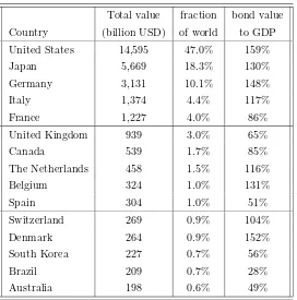
This section will give an overview of the bond and money markets across the world. Let us first look at some summary statistics of the size of the bond markets of the world. Table 1.1 gives a ranking of the world bond markets according to the value of the bonds at the beginning of 2000. By far the largest bond market is the U.S. market with a value of 14,595 billions of US dollars (i.e. 14,595,000,000,000 US dollars), followed by Japan, Canada, and a number of Western European countries. It is also clear from the table that the size of the bond market relative to GDP varies significantly across countries. According to Dimson, Marsh, and Staunton (2002, Fig. 2-2), the bond market is larger than the stock market in Denmark, Germany, Italy, Belgium, and Japan. The value of the U.S. bond market equals 88% of the U.S. stock market. (These observations are based on data from the beginning of 2000.)

(22)

Total value fraction bond value

Country (billion USD) of world to GDP

United States 14,595 47.0% 159%

Japan 5,669 18.3% 130%

Germany 3,131 10.1% 148%

Italy 1,374 4.4% 117%

France 1,227 4.0% 86%

United Kingdom 939 3.0% 65%

Canada 539 1.7% 85%

The Netherlands 458 1.5% 116%

Belgium 324 1.0% 131%

Spain 304 1.0% 51%

Switzerland 269 0.9% 104%

Denmark 264 0.9% 152%

South Korea 227 0.7% 56%

Brazil 209 0.7% 28%

[image:22.612.165.437.44.319.2]

Australia 198 0.6% 49%

Table 1.1: The 15 most valuable bond markets as of the beginning of the year 2000. Source: Table 2-2 in Dimson, Marsh, and Staunton (2002).

associations are often also traded. The bonds issued in a given national market must comply with the regulation of that particular country. Bonds issued in the less regulated Eurobond market are usually underwritten by an international syndicate and offered to investors in several coun-tries simultaneously. Many Eurobonds are listed on one national exchange, often in Luxembourg or London, but most of the trading in these bonds takes place OTC (over-the-counter). Other Eurobonds are issued as a private placement with financial institutions. Eurobonds are typically issued by international institutions, governments, or large multi-national corporations.

The Bank for International Settlements (BIS) publishes regularly statistics on financial markets across the world. BIS distinguishes between domestic debt and international debt securities. The term “debt securities” covers both bonds and money market contracts. The term “domestic” means that the security is issued in the local currency by residents in that country and targeted at resident investors. All other debt securities are classified by BIS as “international.” Based on BIS statistics published in Bank for International Settlements (2004), henceforth referred to as BIS (2004), Table 1.2 ranks domestic markets for debt securities according to the amounts outstanding in June 2004. There are only small differences in the rankings of Table 1.1 and 1.2.

(23)

fraction of domestic market

Amounts outstanding fraction financial corporate

Country (billion USD) of world governments institutions issuers

United States 18,135 44.3% 29.1% 56.7% 14.1%

Japan 8,317 20.3% 76.3% 14.6% 9.1%

Italy 2,130 5.2% 64.7% 25.4% 10.0%

Germany 2,014 4.9% 51.4% 43.2% 5.4%

France 1,869 4.6% 56.0% 31.1% 12.8%

United Kingdom 1,416 3.5% 42.6% 28.0% 29.4%

Spain 709 1.7% 56.9% 24.1% 19.0%

Canada 685 1.7% 73.4% 14.1% 12.6%

The Netherlands 590 1.4% 44.2% 45.8% 10.1%

South Korea 488 1.2% 29.8% 39.4% 30.8%

China 442 1.1% 65.0% 32.2% 2.8%

Belgium 431 1.1% 72.6% 19.3% 8.0%

Denmark 369 0.9% 29.5% 65.4% 5.2%

Brazil 295 0.7% 80.6% 18.5% 0.9%

Australia 294 0.7% 28.0% 43.4% 28.6%

[image:23.612.58.488.48.352.2]

All countries 40,869 100.0% 48.6% 38.7% 12.8%

Table 1.2: The largest domestic markets for debt securities divided by issuer category as of June 2004. Source: Tables 16A-B in BIS (2004).

debt securities, but the U.S. dollar is also used very often.

The Tables 1.2 and 1.3 split up the different markets according to three categories of issuers: governments, financial institutions, and corporate issuers. On average, close to 49% of the debt securities traded in domestic markets are issued by governments, 39% by financial institutions, and 13% by corporate issuers. In contrast, the international markets are dominated by financial institutions who stand behind approximately 74% of the issues, 12% are issued by corporations, 10% by governments, and 4% by international organizations. Again, we see large difference across countries. Let us look more closely at the different issuers and the type of debt securities they typically issue.

(24)

by residence of issuer by nationality of issuer

bonds, money bonds, money govern- financial corporate

Country total notes market total notes market ments institut. issuers

United States 3,214 3,169 45 3,196 3,118 78 0.1% 87.6% 12.3%

United Kingdom 1,446 1,285 160 1,241 1,141 100 0.3% 83.1% 16.6%

Germany 1,442 1,364 77 2,022 1,880 142 7.9% 88.1% 4.0%

The Netherlands 949 892 56 608 552 56 0.2% 89.9% 9.9%

France 763 727 37 778 743 36 2.5% 67.2% 30.3%

Cayman Islands 476 446 29 27 24 3 0.0% 100.0% 0.0%

Italy 455 452 3 585 565 20 31.0% 59.6% 9.4%

Spain 290 289 1 436 425 11 11.4% 82.4% 6.2%

Canada 282 279 3 269 266 3 32.0% 33.3% 34.7%

Australia 253 207 45 210 187 24 5.7% 87.3% 7.1%

Japan 133 132 1 284 267 17 1.4% 78.0% 20.6%

Belgium 114 97 17 256 237 19 28.0% 68.3% 3.7%

Int. organizations 517 513 3 517 513 3 NA NA NA

[image:24.612.87.581.71.343.2]

All countries 12,337 11,740 598 12,337 11,740 598 10.0% 73.7% 12.1%

Table 1.3: International debt securities by residence and nationality of issuer as of June 2004. The numbers are amounts outstanding in billions of USD. The list includes countries that are in the top 10 either by residence of issuer or nationality of issuer. Source: Tables 11, 12A-D, 14A-B, 15A-B in BIS (2004).

Currency bonds and notes money market

Euro 5,127 275

US dollar 4,709 182

Pound sterling 859 85

Yen 504 16

Swiss franc 200 17

Australian dollar 97 7

Canadian dollar 86 2

Hong Kong dollar 50 9

Other currencies 108 5

Total 11,740 598

[image:24.612.172.428.466.649.2]

(25)

when first issued. Treasury notes are issued with a time-to-maturity of 1-10 years, while Treasury bonds mature in more than 10 years and up to 30 years from their issue date. The Treasury sells two types of notes and bonds, fixed-principal and inflation-indexed. The fixed-principal type promises given dollar payments in the future, whereas the dollar payments of the inflation-indexed type are adjusted to reflect inflation in consumer prices.1 _{Finally, the U.S. Treasury also issue}

so-calledsavings bondsto individuals and certain organizations, but these bonds are not subsequently tradable.

While Treasury notes and bonds are issued as coupon bonds, the Treasury Department in-troduced the so-called STRIPS program in 1985 that lets investors hold and trade the individual interest and principal components of most Treasury notes and bonds as separate securities.2 _These

separate securities, which are usually referred to as STRIPs, are zero-coupon bonds. Market par-ticipants create STRIPs by separating the interest and principal parts of a Treasury note or bond. For example, a 10-year Treasury note consists of 20 semi-annual interest payments and a principal payment payable at maturity. When this security is “stripped”, each of the 20 interest payments and the principal payment become separate securities and can be held and transferred separately.3 In some countries including the U.S., bonds issued by various public institutions, e.g. utility companies, railway companies, export support funds, etc., are backed by the government, so that the default risk on such bonds is the risk that the government defaults. In addition, some bonds are issued by government-sponsored entities created to facilitate borrowing and reduce borrowing costs for e.g. farmers, homeowners, and students. However, these bonds are typically not backed by the government and are therefore exposed to the risk of default of the issuing organization. Bonds may also be issued by local governments. In the U.S. such bonds are known as municipal bonds.

In the United States, the United Kingdom, and some other countries, corporations will tra-ditionally raise large amounts of capital by issuing bonds, so-calledcorporate bonds. In other countries, e.g. Germany and Japan, corporations borrow funds primarily through bank loans, so that the market for corporate bonds is very limited. For corporate bonds, investors cannot ignore the possibility that the issuer defaults and cannot meet the obligations represented by the bonds. Bond investors can either perform their own analysis of the creditworthiness of the issuer or rely on the analysis of professional rating agencies such as Moody’s Investors Service or Standard & Poor’s Corporation. These agencies designate letter codes to bond issuers both in the U.S. and in other countries. Investors will typically treat bonds with the same rating as having (nearly) the same default risk. Due to the default risk, corporate bonds are traded at lower prices than sim-ilar (default-free) government bonds. The management of the issuing corporation can effectively transfer wealth from bond-holders to equity-holders, e.g. by increasing dividends, taking on more risky investment projects, or issuing new bonds with the same or even higher priority in case of default. Corporate bonds are often issued with bond covenants or bond indentures that restrict

1_{The principal value of an inflation-indexed note or bond is adjusted before each payment date according to the} change in the consumer price index. Since the semi-annual interest payments are computed as the product of the fixed coupon rate and the current principal, all the payments of an indexed note or bond are inflation-adjusted.

2_{STRIPS is short for Separate Trading of Registered Interest and Principal of Securities.}

(26)

management from implementing such actions.

U.S. corporate bonds are typically issued with maturities of 10-30 years and are often callable bonds, so that the issuer has the right to buy back the bonds on certain terms (at given points in time and for a given price). Some corporate bonds are convertible bonds meaning that the bond-holders may convert the bonds into stocks of the issuing corporation on predetermined terms. Although most corporate bonds are listed on a national exchange, much of the trading in these bonds is in the OTC market.

When commercial banks and other financial institutions issue bonds, the promised payments are sometimes linked to the payments on a pool of loans that the issuing institution has provided to households or firms. An important example is the class of mortgage-backed bonds which constitutes a large part of some bond markets, e.g. in the U.S., Germany, Denmark, Sweden, and Switzerland. A mortgage is a loan that can (partly) finance the borrower’s purchase of a given real estate property, which is then used as collateral for the loan. Mortgages can be residential (family houses, apartments, etc.) or non-residential (corporations, farms, etc.). The issuer of the loan (the lender) is a financial institution. Typical mortgages have a maturity between 15 and 30 years and are annuities in the sense that the total scheduled payment (interest plus repayment) at all payment dates are identical. Fixed-rate mortgages have a fixed interest rate, while adjustable-rate mortgages have an interest rate which is reset periodically according to some reference rate. A characteristic feature of most mortgages is the prepayment option. At any payment date in the life of the loan, the borrower has the right to pay off all or part of the outstanding debt. This can occur due to a sale of the underlying real estate property, but can also occur after a drop in market interest rates, since the borrower then have the chance to get a cheaper loan.

Mortgages are pooled either by the issuers or other institutions, who then issue mortgage-backed securities that have an ownership interest in a given pool of mortgage loans. The most common type of mortgage-backed securities is the so-called pass-through, where the pooling institution simply collects the payments from borrowers with loans in a given pool and “passes through” the cash flow to investors less some servicing and guaranteeing fees. Many pass-throughs have payment schemes equal to the payment schemes of bonds, e.g. pass-throughs issued on the basis of a pool of fixed-rate annuity mortgage loans have a payment schedule equal to that of annuity bond. However, when borrowers in the pool prepay their mortgage, these prepayments are also passed through to the security-holders, so that their payments will be different from annuities. In general, owners of pass-through securities must take into account the risk that the mortgage borrowers in the pool default on their loans. In the U.S. most pass-throughs are issued by three organizations that guarantee the payments to the securities even if borrowers default. These organizations are the Government National Mortgage Association (called “Ginnie Mae”), the Federal Home Loan Mortgage Corporation (“Freddie Mac”), and the Federal National Mortgage Association (“Fannie Mae”). Ginnie Mae pass-throughs are even guaranteed by the U.S. government, but the securities issued by the two other institutions are also considered virtually free of default risk.

(27)

1.4 Fixed income derivatives 15

six months. Interest rates set on deposits at the London interbank market are called LIBOR rates (LIBOR is short for London Interbank offered rate).

To manage very short-term liquidity, financial institutions often agree on overnight loans, so-called federal funds. The interest rate charged on such loans is called the Fed funds rate. The Federal Reserve has a target Fed funds rate and buys and sells securities in open market operations to manage the liquidity in the market, thereby also affecting the Fed funds rate. Banks may obtain temporary credit directly from the Federal Reserve at the so-called “discount window”. The interest rate charged by the Fed on such credit is called the federal discount rate, but since such borrowing is quite uncommon nowadays, the federal discount rate serves more as a signaling device for the targets of the Federal Reserve.

Large corporations, both financial corporations and others, often borrow short-term by issuing so-calledcommercial papers. Another standard money market contract is a repurchase agreement or simplyrepo. One party of this contract sells a certain asset, e.g. a short-term Treasury bill, to the other party and promises to buy back that asset at a given future date at the market price at that date. A repo is effectively a collateralized loan, where the underlying asset serves as collateral. As central banks in other countries, the Federal Reserve in the U.S. participates actively in the repo market to implement their monetary policy. The interest rate on repos is called the repo rate. More details on U.S. bond markets can be found in e.g. Fabozzi (2000), while Batten, Fether-ston, and Szilagyi (2004) contains detailed information on European bond and money markets.

1.4 Fixed income derivatives

A wide variety of fixed income derivatives are traded around the world. In this section we provide a brief introduction to the markets for such securities. In the pricing models we develop in later chapters we will look for prices of some of the most popular fixed income derivatives. Chapter 6 contains more details on a number of fixed income derivatives, what cash flow they offer, how the different derivatives are related, etc.

Aforwardis the simplest derivative. A forward contract is an agreement between two parties on a given transaction at a given future point in time and at a price that is already fixed when the agreement is made. For example, a forward on a bond is a contract where the parties agree to trade a given bond at a future point in time for a price which is already fixed today. This fixed price is usually set so that the value of the contract at the time of inception is equal to zero so that no money changes hand before the delivery date. A closely related contract is the so-called forward rate agreement (FRA). Here the two parties agree upon that one party will borrow money from the other party over some period beginning at a given future date and the interest rate for that loan is fixed already when this FRA is entered. In other words, the interest rate for the future period is locked in. FRAs are quite popular instruments in the money markets.

(28)

was originally taken. Futures on government bonds are traded at many leading exchanges. A very popular exchange-traded derivative is the so-called Eurodollar futures, which is basically the futures equivalent of a forward rate agreement.

Anoptiongives the holder the right to make some specified future transaction at terms that are already fixed. A call option gives the holder the right to buy a given security at a given price at or before a given date. Conversely, a put option gives the holder the right to sell a given security. If the option gives the right to make the transaction at only one given date, the option is said to be European-style. If the right can be exercised at any point in time up to some given date, the option is said to be American-style. Both European- and American-style options are traded. Options on government bonds are traded at several exchanges and also on the OTC-markets. In addition, many bonds are issued with “embedded” options. For example, many mortgage-backed bonds and corporate bonds are callable, in the sense that the issuer has the right to buy back the bond at a pre-specified price. To value such bonds, we must be able to value the option element.

Various interest rate options are also traded in the fixed income markets. The most popular are caps and floors. A cap is designed to protect an investor who has borrowed funds on a floating interest rate basis against the risk of paying very high interest rates. Therefore the cap basically gives you the right to borrow at some given rate. A cap can be seen as a portfolio of interest rate call options. Conversely, a floor is designed to protect an investor who has lent funds on a floating rate basis against receiving very low interest rates. A floor is a portfolio of interest rate put options. Various exotic versions of caps and floors are also quite popular.

Answapis an exchange of two cash flow streams that are determined by certain interest rates. In the simplest and most common interest rate swap, aplain vanillaswap, two parties exchange a stream of fixed interest rate payments and a stream of floating interest rate payments. There are also currency swaps where streams of payments in different currencies are exchanged. In addition, many exotic swaps with special features are widely used. The international OTC swap markets are enormous, both in terms of transactions and outstanding contracts.

Aswaptionis an option on a swap, i.e. it gives the holder the right, but not the obligation, to enter into a specific swap with pre-specified terms at or before a given future date. Both European-and American-style swaptions are traded.

The Bank for International Settlements (BIS) also publishes statistics on derivative trading around the world. Table 1.5 provide some interesting statistics on the size of derivatives markets at organized exchanges. The markets for interest rate derivatives are much larger than the markets for currency- or equity-linked derivatives. The option markets generally dominate futures markets measured by the amounts outstanding, but ranked according to turnover futures markets are larger than options markets.

(29)

1.5 An overview of the book 17

Instruments/ Futures Options

Location Amount outstanding Turnover Amount outstanding Turnover

All markets 17,662 213,455 31,330 75,023

Interest rate 17,024 202,064 28,335 63,548

Currency 84 1,565 37 120

Equity index 553 9,827 2,958 11,355

North America 9,778 122,516 18,120 49,278

Europe 5,534 77,737 12,975 19,693

Asia-Pacific 2,201 11,781 170 5,786

[image:29.612.122.422.285.389.2]

Other markets 149 1,421 66 266

Table 1.5: Derivatives traded on organized exchanges. All amounts are in billions of US dollars. The amount outstanding is of September 2004, while the turnover figures are for the third quarter of 2004. Source: Table 23A in BIS (2004).

Maturity in years

Contracts total

≤1 1–5 _≥5

All interest rate 164,626 57,157 66,093 41,376

Forward rate agreements 13,144

Swaps 127,570 49,397 56,042 35,275

Options 23,912 7,760 10,052 6,101

Table 1.6: Amounts outstanding (billions of US dollars) on OTC single-currency interest rate derivatives as of June 2004. Source: Tables 21A and 21C in BIS (2004).

7% in pound sterling, cf. Table 21B in BIS (2004).

1.5 An overview of the book

We want to understand the dynamics of interest rates and the prices of fixed income securities. The key element in our analysis will be the term structure of interest rates. The cleanest picture of the link between interest rates and maturities is given by a zero-coupon yield curve. Since only few zero-coupon bonds are traded, we have to extract an estimate of the zero-coupon yield curve from prices of the traded coupon bonds. We will discuss methods for doing that in Chapter 2.

Since future values of most relevant variables are uncertain, we have to model the behavior of uncertain variables or objects over time. This is done in terms of stochastic processes. A stochastic process is basically a collection of random variables, namely one random variable for each of the points in time at which we are interested in the value of this object. To understand and work with modern fixed income models therefore requires some knowledge about stochastic processes, their properties, and how to do relevant calculations involving stochastic processes. Chapter 3 provides the information about stochastic processes that is needed for our purposes.

(30)

income securities follows the same general principles as the pricing of all other financial assets. Chapter 4 reviews some of the important results on asset pricing theory. In particular, we define and relate the key concepts of arbitrage, state-price deflators, and risk-neutral probability measures. The connections to market completeness and individual investors’ behavior are also addressed. Furthermore, we consider the special class of diffusion models. All these results will be applied in the following chapters to the term structure of interest rate and the pricing of fixed income securities.

In Chapter 5 we study the links between the term structure of interest rates and macro-economic variables such as aggregate consumption, production, and inflation. The term structure of interest rates reflects the prices of bonds of various maturities and, as always, prices are set to align supply and demand. An individual or corporation that has a clear preference for current capital to finance investments or current consumption can borrow by issuing a bond to an individual who has a clear preference for future consumption opportunities. The price of a bond of a given maturity will therefore depend on the attractiveness of the real investment opportunities and on the individuals’ preferences for consumption over the maturity of the bond. Following this intuition we develop relations between interest rates, aggregate consumption, and aggregate production. We also explore the relations between nominal interest rates, real interest rates, and inflation. Finally, the chapter reviews some of the traditional hypotheses on the shape of the yield curve, e.g. the expectation hypotheses, and discuss their relevance (or, rather, irrelevance) for modern fixed income analysis. Chapter 6 provides an overview of the most popular fixed income derivatives, e.g. futures and options on bonds, Eurodollar futures, caps and floors, and swaps and swaptions. We will look at the characteristics of these securities and what we can say about their prices without setting up any concrete term structure model.

Starting with Chapter 7 we focus on dynamic term structure models developed for the pricing of fixed income securities and the management of interest rate risk. Chapter 7 goes through so-called one-factor diffusion models. This type of models was the first to be applied in the literature and dates back at least to 1970. The one-factor models of Vasicek and Cox, Ingersoll, and Ross are still frequently applied both in practice and in academic research. They have a lot of realistic features and deliver relatively simple pricing formulas for many fixed income securities. Chapter 8 explores multi-factor models which have several advantages over one-factor models, but are also more complicated to analyze and apply.

The diffusion models deliver prices both for bonds and derivatives. However, the model price for a given bond may not be identical to the actually observed price of the bond. If you want to price a derivative on that bond, this seems problematic. If the model does not get the price of the underlying security right, why trust the models price of the derivative? In Chapter 9 we discuss how one- and multi-factor models can be extended to be consistent with current market information, such as bond prices and volatilities. A more direct route to ensuring consistency is explored in Chapter 10 that introduces and analyzes so-called Heath-Jarrow-Morton models. They are characterized by taking the current market term structure of interest rates as given and then modeling the evolution of the entire term structure in an arbitrage-free way. We will explore the relation between these models and the factor models studied in earlier chapters.

(31)

1.6 Exercises 19

markets, namely caps, floors, and swaptions. These models have become increasingly popular in recent years.

In Chapters 6–11 we focus on the pricing of various fixed income securities. However, it is also extremely important to be able to measure and manage interest rate risk. Interest rate risk measures of individual securities are needed in order to obtain an overview of the total interest rate risk of the investors’ portfolio and to identify the contribution of each security to this total risk. Many institutional investors are required to produce such risk measures for regulatory authorities and for publication in their accounting reports. In addition, such risk measures constitute an important input to the portfolio management. Interest rate risk management is the topic of Chapter 12. First, some traditional interest rate risk measures are reviewed and criticized. Then we turn to risk measures defined in relation to the dynamic term structure models studied in the previous chapters.

The following chapters deal with some securities that require special attention. The subject of Chapter 13 is how to construct models for the pricing and risk management of mortgage-backed securities. The main concern is how to adjust the models studied in earlier chapters to take the prepayment options involved in mortgages into account. In Chapter 14 (only some references are listed in the current version) we discuss the pricing of corporate bonds and other fixed income securities where the default risk of the issuer cannot be ignored. Chapter 15 focuses on the consequences that stochastic variations in interest rates have for the valuation of securities with payments that are not directly related to interest rates, such as stock options and currency options. Finally, Chapter 16 (only some references are listed in the current version) describes several numerical techniques that can be applied in cases where explicit pricing and hedging formulas are not available.

1.6 Exercises

EXERCISE 1.1_{Show that if the discount function does}not satisfy the condition

BtT≥BtS, T < S,

then negative forward rates will exist. Are non-negative forward rates likely to exist? Explain!

EXERCISE 1.2_{Consider two bullet bonds, both with annual payments and exactly four years to}

ma-turity. The first bond has a coupon rate of 6% and is traded at a price of 101.00. The other bond has a

coupon rate of 4% and is traded at a price of 93.20. What is the four-year discount factor? What is the

(32)

(33)

Chapter 2

Extracting yield curves from bond prices

2.1 Introduction

As discussed in Chapter 1, the clearest picture of the term structure of interest rates is obtained by looking at the yields of zero-coupon bonds of different maturities. However, most traded bonds are coupon bonds, not zero-coupon bonds. This chapter discusses methods to extract or estimate a zero-coupon yield curve from the prices of coupon bonds at a given point in time.

Section 2.2 considers the so-called bootstrapping technique. It is sometimes possible to con-struct zero-coupon bonds by forming certain portfolios of coupon bonds. If so, we can deduce an arbitrage-free price of the zero-coupon bond and transform it into a zero-coupon yield. This is the basic idea in the bootstrapping approach. Only in bond markets with sufficiently many coupon bonds with regular payment dates and maturities can the bootstrapping approach deliver a decent estimate of the whole zero-coupon yield curve. In other markets, alternative methods are called for.

We study two alternatives to bootstrapping in Sections 2.3 and 2.4. Both are based on the assumption that the discount function is of a given functional form with some unknown parameters. The value of these parameters are then estimated to obtain the best possible agreement between observed bond prices and theoretical bond prices computed using the functional form. Typically, the assumed functional forms are either polynomials or exponential functions of maturity or some combination. This is consistent with the usual perception that discount functions and yield curves are continuous and smooth. If the yield for a given maturity was much higher than the yield for another maturity very close to the first, most bond owners would probably shift from bonds with the low-yield maturity to bonds with the high-yield maturity. Conversely, bond issuers (borrowers) would shift to the low-yield maturity. These changes in supply and demand will cause the gap between the yields for the two maturities to shrink. Hence, the equilibrium yield curve should be continuous and smooth. The unknown parameters can be estimated by least-squares methods.

We focus here on two of the most frequently applied parameterization techniques, namely cubic splines and the Nelson-Siegel parameterization. An overview of some of the many other approaches suggested in the literature can be seen in Anderson, Breedon, Deacon, Derry, and Murphy (1996, Ch. 2). For some recent procedures, see Jaschke (1998) and Linton, Mammen, Nielsen, and Tanggaard (2001).

(34)

2.2 Bootstrapping

In many bond markets only very few zero-coupon bonds are issued and traded. (All bonds issued as coupon bonds will eventually become a zero-coupon bond after their next-to-last payment date.) Usually, such zero-coupon bonds have a very short maturity. To obtain knowledge of the market zero-coupon yields for longer maturities, we have to extract information from the prices of traded coupon bonds. In some markets it is possible to construct some longer-term zero-coupon bonds by forming portfolios of traded coupon bonds. Market prices of these “synthetical” zero-coupon bonds and the associated zero-coupon yields can then be derived.

Example 2.1Consider a market where two bullet bonds are traded, a 10% bond expiring in one year and a 5% bond expiring in two years. Both have annual payments and a face value of 100. The one-year bond has the payment structure of a zero-coupon bond: 110 dollars in one year and nothing at all other points in time. A share of 1/110 of this bond corresponds exactly to a zero-coupon bond paying one dollar in a year. If the price of the one-year bullet bond is 100, the one-year discount factor is given by

Btt+1= 1

110·100≈0.9091.

The two-year bond provides payments of 5 dollars in one year and 105 dollars in two years. Hence, it can be seen as a portfolio of five one-year zero-coupon bonds and 105 two-year zero-coupon bonds, all with a face value of one dollar. The price of the two-year bullet bond is therefore

B2,t= 5Btt+1+ 105Btt+2,

cf. (1.4). IsolatingBtt+2, we get

Btt+2= 1

105B2,t− 5 105B

t+1

t . (2.1)

If for example the price of the two-year bullet bond is 90, the two-year discount factor will be

Btt+2= 1 105 ·90−

5

105 ·0.9091≈0.8139.

From (2.1) we see that we can construct a two-year zero-coupon bond as a portfolio of 1/105 units of the two-year bullet bond and−5/105 units of the one-year zero-coupon bond. This is equivalent to a portfolio of 1/105 units of the two-year bullet bond and₋5/(105_·110) units of the one-year bullet bond. Given the discount factors, zero-coupon rates and forward rates can be calculated as

shown in Section 1.2. 2

The example above can easily be generalized to more periods. Suppose we have M bonds with maturities of 1,2, . . . , M periods, respectively, one payment date each period and identical payment date. Then we can construct successively zero-coupon bonds for each of these maturities and hence compute the market discount factors Btt+1, Btt+2, . . . , Btt+M. First, Btt+1 is computed using the shortest bond. Then,Btt+2 is computed using the next-to-shortest bond and the already computed value of Btt+1, etc. Given the discount factors Btt+1, Btt+2, . . . , Btt+M, we can compute the zero-coupon interest rates and hence the zero-coupon yield curve up to timet+M (for theM