Nonconservative Robust Control: Optimized and
Constrained Sensitivity Functions
Carl-Magnus Fransson, Torsten Wik, Bengt Lennartson, Michael Saunders, and
Per-Olof Gutman
, Senior Member, IEEE
Abstract—An automated procedure for optimization of pro-portional–integral–derivative (PID)-type controller parameters for single-input, single-output (SISO) plants with explicit model uncertainty is presented. Robustness to the uncertainties is guar-anteed by the use of Horowitz–Sidi bounds, which are used as constraints when low-frequency performance is optimized in a nonconvex but smooth optimization problem. In the optimization (and hence the parameter tuning), separate criteria are formulated for low-, mid-, and high-frequency (HF) closed-loop properties. The tradeoff between stability margins, control signals, HF ro-bustness, and low-frequency performance is clarified, and the final parameter choice is facilitated. We use a combination of global and local optimization algorithms in the TOMLAB optimization environment and obtain robust convergence without relying on good initial estimates for the controller parameters. The method is applied to a controller structure comparison for a plant with an uncertain mechanical resonance and a plant with uncertain time delay and time constants. For a given control activity, stability margin, and HF robustness, it is shown that a PID controller with a second-order filter and an controller based on loop-shaping achieve approximately the same low-frequency performance.
Index Terms—Control systems, convergence of numerical methods, control, optimal control, optimization methods, process control, proportional control, robustness.
I. INTRODUCTION
I
N MANY controller design techniques, a mixed, possibly weighted, performance criterion is used to ensure that the closed loop achieves desirable behavior. The criterion includes multiple closed-loop objectives and is minimized to obtain a so-lution optimal with respect to the weighted performance objec-tives (as in mixed-sensitivity optimization). However, by con-sidering separate criteria at different frequency regions, instead of aggregating the closed-loop properties into a single criterion,Manuscript received June 24, 2003; revised February 20, 2008. Manu-script received in final form April 03, 2008. First published June 24, 2008; current version published February 25, 2009. Recommended by Associate Editors M. Skliar and F. Doyle.
C.-M. Fransson, deceased, was with the Department of Signals and Systems, Chalmers University of Technology, SE 412 96 Göteborg, Sweden.
T. Wik and B. Lennartson are with the Department of Signals and Systems, Chalmers University of Technology, SE 412 96 Göteborg, Sweden (e-mail: [email protected]; [email protected]).
M. Saunders is with the Systems Optimization Laboratory, Department of Management Science and Engineering, Stanford University, Stanford, CA 94305-4026 USA (e-mail: [email protected]).
P.-O. Gutman is with the Faculty of Civil and Environmental Engineering, Technion—Israel Institute of Technology, Haifa 32000, Israel (e-mail: [email protected]).
Digital Object Identifier 10.1109/TCST.2008.924564
the tradeoff between performance and robustness can be evalu-ated, especially in the case of a change of closed-loop specifi-cations. Such a procedure has been demonstrated for the tuning of PI and proportional–integral–derivative (PID) controllers by optimization when no uncertainties are considered [1], [2].
For plants with uncertainties, the mid-frequency (MF) ro-bustness properties are crucial. Particularly within process con-trol, where plant uncertainties can be large, integral action is common, and then the low-frequency (LF) performance and ro-bustness are less affected by the uncertainties [15]. For high fre-quencies (HF), good performance and robustness are simply a question of having a small loop gain. If explicit descriptions of the plant uncertainties have been formulated, the quantitative feedback theory (QFT) [3] can be used to design controllers such that specified bounds on the magnitudes of the sensitivity function and the control sensitivity function (for example) are satisfied in spite of the uncertainties. The basis for this method is a translation of the constraints on and to so-called Horowitz–Sidi bounds on the nominal open loop. For this purpose, a toolbox QSYN [4] running on MATLAB[5] can be used.
The traditional QFT design method aims to minimize the HF open-loop gain [6], [7]. It assumes no fixed structure of the con-troller and gives, in its general form, an unlimited number of tuning parameters. However, the QFT approach can be applied to fixed structure controllers, such as in [8], where it was ap-plied to an ideal PID controller. The procedure uses bounds on the complementary sensitivity when minimizing the derivative gain. The basis for the method is a simplification of the op-timization using the fact that by specifying the phase of the compensator for two frequencies, the phase is defined for all frequencies because it only depends on two parameters (inte-gral time and derivative time). This method is extended in [9] to two other three-parameter compensators. Yaniv and Nagurka [10] have also developed an optimization method restricted to three-parameter PID controllers, but for the case when the phase margin is specified and one sensitivity function is bounded. The problem can then be formulated to rely on (repeated) solutions to fouth-order polynomials, which appears to avoid the problem of local minima. To deal with uncertainties other than gain un-certainty, the problem must still be solved for every chosen fre-quency and plant parameter value.
Garciaet al.[11] describe a method for PID tuning for un-certain plants that considers multiple frequency-domain closed-loop measures. However, the optimization is based on a standard Gauss–Newton algorithm and suffers from problems of local optima. The optimized criterion used is also a weighted
sum of squared frequency characteristics, and unstructured disc uncertainties are used to modify the modulus margins to make the design robust.
All of the above methods need frequency gridding to be solved numerically, with a consequent increase in compu-tational effort with gridding density. By use of the Kalman Yacubovich-Popov lemma, Hara et al. [12] transform fre-quency-domain constraints on PIDs into linear matrix in-equalities (LMIs) and then avoid the approximations caused by frequency gridding. However, the design is by open-loop shaping and does not apply directly to closed-loop specifica-tions. When applied to plants with parametric uncertainties, the problem is still transformed into an LMI optimization problem albeit with potential conservatism.
Neither the QFT-based methods [6]–[9] nor the other recent methods discussed [10]–[12] consider the general tradeoff between the LF, MF, and HF properties of the closed loop. This tradeoff is important because the process disturbance rejection, for example, can often be significantly improved at only a mar-ginal reduction of the HF robustness [13], [14]. To pursue this, Franssonet al.developed a constrained optimization procedure where PID and PID weighted loop-shaping controllers were designed based on an optimization of the LF performance subject to specified bounds on the maximum sensitivity and the maximum nominal control sensitivity [15], [16]. Robustness of the sensitivity function to plant uncertainties was guaranteed by Horowitz–Sidi bounds, but the procedure suffered from the fact that local optimization methods were used to solve highly nonlinear problems with potential discontinuities in the param-eter space. As a result, difficulties were frequently experienced with initial guesses, convergence, and local optima.
In [17], the design procedure in [15] and [16] was generalized to include robustness to plant model uncertainties for the control sensitivity function, and a global optimization algorithm was applied to the design problem. This paper summarizes earlier work by the authors [15]–[17] and improves the methods used in the following ways.
• The numerical treatment for solving the design problem is improved, which results in fast convergence towards a globally optimal controller (of a fixed structure).
• A reliable test is given that determines if the nominal loop transfer function is (pointwise) inside or outside the Horowitz–Sidi bounds in the Nichols chart.
• In the evaluation procedure, closed-loop properties (in terms of stability robustness, control activity, and high-fre-quency (HF) robustness) are constrained identically in the comparison of low-frequency performance.
[image:2.594.355.499.65.117.2]The suggested approach applies to fixed structure controllers in general, with multiple closed-loop sensitivity constraints, and there is no theoretical limitation in the number of controller pa-rameters. Basically, the same optimization problem, i.e., min-imization of a low-frequency performance criterion subject to bounds on additional performance and robustness measures, has been solved for multiple-input, multiple-output (MIMO) sys-tems by the authors, using the structured singular value [18]. The same methods may naturally be applied to single-input, single-output (SISO) systems as well. However, for many SISO cases, the QFT-based method presented here is superior to the
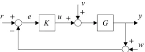
Fig. 1. Closed-loop system.
use of structured singular values [19]. For systems where the same uncertain parameter occurs in many places of a system model, the dimension of the nominal closed-loop system matrix , resulting from linear fractional transformations, may be-come very large. This can make structured singular value deter-minations unfeasible, while the method presented here is quite insensitive to this [19].
This paper is organized as follows. In Section II, we define frequency-domain closed-loop performance measures and de-scribe how they are used to pose the design problem. Section III presents the controller structures used, and Section IV discusses how robustness to plant model uncertainties can be ensured by use of the Horowitz–Sidi test. Section V details the numerical treatment of the method and we give an algorithm for solving the design problem. The method is illustrated by two examples in Section VI, and Section VII summarizes and concludes the paper.
II. CONTROLPROBLEM
A. Robustness and Performance Measures
It is well known that improvement of a controller design in one respect will often cause deterioration in another respect. Different closed-loop properties, such as stability, tracking, dis-turbance attenuation, and the magnitude of the control signals due to reference steps or disturbances, are often related to dif-ferent frequency ranges of the closed loop and are not inde-pendent of each other. Therefore, a method for comparing con-trollers with each other should have the property that important closed-loop properties not immediately compared are identi-cally constrained for all controllers. The method presented here fulfills this demand. It is based on four measures [13], each of them related to essential performance and robustness qualities of the closed loop and also roughly related to different frequency ranges as follows:
where denotes the plant, denotes the controller, is the sensitivity function, and represents the roll-off rate of the controller (see Fig. 1).
is a measure of the control activity due to measurement noise, related to the MF and HFy region around (or somewhat above) the closed-loop bandwidth. is a measure of the robustness to unmodelled dynamics in the HF region. Recall the small gain theorem and the fact that is related to the complementary sensitivity function as . Then, for a proper (but not strictly proper) controller, such as a PID controller with a first-order filter, , and hence
.
Each of the presented measures relates to a different region of the frequency range (LF, MF, and HF). Thus, simultaneous use of these measures in a design procedure facilitates determina-tion of controllers that give acceptable behavior of the closed-loop system for all frequencies. However, since the plant is as-sumed to be uncertain, all of the measures above will be func-tions of the plant uncertainty.
B. Plant Uncertainty
An uncertain plant transfer function can be defined as a member of a set of transfer functions [4]
where the set may contain finitely or infinitely many plant cases. By defining a set of frequencies as , we have that for each frequency , the set in the complex plane is called atemplate, or value set, for [3]. The template should enclose all possible frequency responses of the plant at the frequency . This paper concerns a special class of uncer-tainty, namely, the parametric plant uncertainty defined by
(1)
where is a vector of uncertain parameters. Thenominalplant is denoted and reflects the choice of a particular .
C. Design Problem
The design problem is posed by incorporating the uncertainty description into the robustness and performance measures. A controller that, despite the uncertainties in the plant, achieves ac-ceptable behavior of the closed-loop system for all frequencies can be obtained by solving the following optimization problem:
(2)
(3)
Thus, is the controller obtained by minimizing the LF performance measure subject to user-defined constraints
, and on and ,
respectively.
D. Simplifications
If a general expression for controllers with integral action is introduced as
(4)
where is bounded, it can readily be shown that
as (provided
[15], [20]. Thus, for PID controllers and SISO systems, the in-verse of the integral gain serves as a close approximation to (this conclusion is based on the fact that good damping—i.e., appropriate stability margin, is assumed). Hence, will be relatively independent of the plant uncertainty. Also, de-pends weakly on the uncertainties, which predominantly affect the mid-frequency region of the closed loop. With this in mind, (2) and (3) can be simplified to
(5)
(6)
where and are based on the nominal plant. If, for some reason, is expected to depend significantly on the uncertain-ties, an approximation of the expected value taking the covari-ance of the parameters into consideration can be used (see [19]).
III. CONTROLLERSTRUCTURES
In this study, both PID controllers and synthesis by shaping [21] are considered when solving (5) and (6). The loop-shaping procedure has the great advantage of not including the -iteration in standard synthesis. Instead, suboptimality is introduced in terms of a scaling factor , which must be properly chosen.
A. PID Controllers
Traditionally, the well-known PID controller, with a first-order filter on the derivative part, used to be formu-lated with the parameters controller gain , integral time , derivative time , and filter constant as
As shown in several papers (e.g., [13]), a PID controller that gives good closed-loop performance and robustness, at least for stable nonoscillating plants, has a complex pair of zeros. This makes it natural to formulate the transfer function of the con-troller as
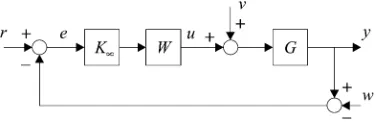
Fig. 2. Closed-loop system with anH loop-shaping controllerKand a plant
G.
where is the integral gain, is the damping ratio, is the inverse of the natural frequency, and is the ratio of the breaking point of the denominator to that of the numerator.
When there is a demand on more HF roll-off in the loop than can be offered by the plant, the PID controller can be augmented by a low-pass filter of arbitrary order. If the first-order filter is exchanged by a filter of second order, the controller can be formulated as
(8)
In Section VI, this controller structure is compared with a PID weighted controller. Note that the roll-off rate of (8) is , and the parameters subject to optimization with (8) are
, and .
B. Loop-Shaping
The first step in the method by Glover and McFarlane [21] is to shape the nominal plant with a weight to give an open loop that meets some nominal performance specifica-tions. For the shaped system , a controller is obtained by solving two Riccati equations. The final
feedback controller for is then (see
Fig. 2). For a given weight , the controller derived in this way will, in some sense, have optimal robustness. The degree of optimality is determined by , where is called the maximum stability margin and is a scaling factor.
In this paper, is parameterized as the PID controller (7) whose parameters ( and ) are subject to tuning by optimization so that a desired closed-loop behavior is obtained. Because of this choice of weight, the final controller will have a roll-off rate , thus explaining the need for using the PID controller with a second-order filter (8) when comparing the PID and controller structures.
IV. HOROWITZ–SIDIBOUNDS
If the plant uncertainty is represented by a set of templates for a number of frequencies, QFT can be used to design a controller such that the closed loop satisfies specifications on the magnitudes of some frequency response functions (such as the sensitivity functions) for all plant variations within a given uncertainty set. The frequency response specifications, in turn, result in constraints on the nominal loop transfer function . These constraints are called Horowitz–Sidi bounds and reflect the interaction between the plant uncertainty and the closed-loop specifications.
We define
where is the uncertain plant and impose an upper bound on the maximum frequency response of this sensitivity function for all plants in , i.e., the following must hold:
(9) Thus, the controller must be chosen such that (9) is fulfilled for the complex numbers . Clearly, for each , there is a set for in the complex plane where (9) does not hold. The union of all such sets give one, or possibly several, sets containing the unacceptable values of . The boundary of this set is called the Horowitz–Sidi bound for with respect to and and is denoted . Multiplying by the nominal plant yields .
The computation of Horowitz–Sidi bounds is done in two steps. The first step demands the computation of the value sets of the plant transfer function. The simplest method is indeed the grid method, where the parameter space is gridded, e.g., equidistantly or randomly, see [22]. More advanced recursive grid or adaptive grid methods exist, see, e.g., [23], where the desired resolution of the computed value set determines the number of grid points, and hence the accuracy of the final result. For special types of transfer functions gridding in the parameter space can be avoided; see [24] and the references therein. Recently, interval analysis has been suggested for value set computation for transfer functions that can be decomposed into elementary functions whose maxima and minima can be analytically calculated [25]. The second step of the computation of Horowitz–Sidi bounds does not require the gridding of the parameter space, but, depending on the desired resolution of the resulting Horowitz–Sidi bound, the gridding of a set in the complex plane.
Horowitz–Sidi bounds can be computed with QSYN [4] and placed in a Nichols chart together with . To ensure that (9) is satisfied for all plants within the uncertainty set, must be shaped so that, at each frequency , it is outside the bound for that frequency (see Fig. 3). Analogously to (9), we also define
(10)
with a corresponding Horowitz–Sidi bound . In an auto-mated procedure, one has to test whether or not is
outside and .
Now, consider a single and transform the origin in the Nichols chart to the interior of the Horowitz–Sidi bound associated with (where the superscript , the subscripts
, and the argument have been dropped for clarity). If is transformed to polar coordinates , we can write , and, if is transformed to the same coordi-nates, it can be represented by . As Fig. 4 illustrates, the test for being outside is then simply
Fig. 3. Nichols chart with Horowitz–Sidi bounds and a nominal open loop for
! = 0:5; 1, and2.
Fig. 4. Nominal open loop and the corresponding Horowitz–Sidi bound for! transformed to polar coordinates.
and the distance in the figure is a measure of how close is to at the frequency . We refer to this as the
Horowitz–Sidi test. Note that the choice of origin is trivial, provided that the nominal case is a member of the template itself. In such a case, the instability point in the Nichols chart is “inside” the Horowitz–Sidi bound. We also note that, for example, the Horowitz–Sidi sensitivity bound will be a single closed curve in the Nichols diagram (the curve may touch itself) if the plant template is simply connected [4]. When the plant template is not simply connected, the Horowitz–Sidi bound can consist of a set of closed curves, and, to handle a situation like this, a different origin for each of the closed curves will have to be chosen.
[image:5.594.58.274.69.240.2]If the choice of origin is bad or is nonconvex, there could be several solutions to , which means that (11) must be modified in order to serve its purpose. Define a crossing between and as a pair of consecutive points and on such that . is then inside if there is an even number of crossings and outside if there is an odd number of crossings, as shown in Fig. 5.
Fig. 5. Illustration of (a) unacceptable and (b) acceptable scenarios when per-forming the Horowitz–Sidi test (11).
V. NONLINEAROPTIMIZATION
Based on the discussion in Section IV, the design problem (5) and (6) can be approximated using (9) and (10) to obtain
(12)
where is the controller parameterization. In the comparison in the next section, the HF-constraint is only used in the op-timization for the controller. is then chosen to be equal to the roll-off of the optimal controller to ensure equal HF robustness of the two controller structures. By use of the Horowitz–Sidi test, (12) is equivalent to
(13)
where the quantities in braces denote the closest distances be-tween the nominal open loop and the Horowitz–Sidi sensitivity bounds and control sensitivity bounds at each frequency.
The optimization problem (13) is smooth but nonconvex. For some initial specifications and , we use a constrained
globaloptimization algorithm, DIRECT [26], to find a set of controller parameters reasonably close to a global optimum
.
Thereafter, we use a gradient-basedlocaloptimizer, SNOPT [27], to obtain more rapid convergence to and to solve a se-quence of nearby problems (13) as and change slowly in a specified pattern.
We summarize the main features of DIRECT and SNOPT before describing the optimization strategy in detail.
A. Global Optimization
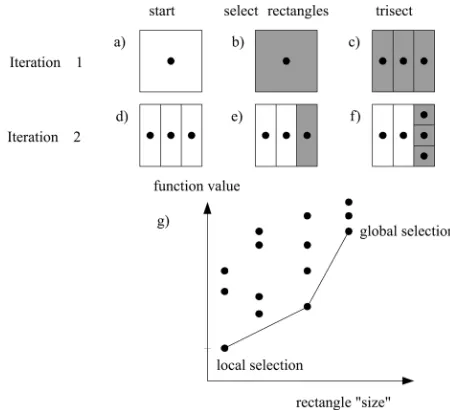
[image:5.594.50.279.301.474.2]Fig. 6. (a)–(f) Two iterations of a 2-D example of the DIRECT algorithm, il-lustrating the partitioning of the search space. (g) Midpoint function values of sampled rectangles (dots) versus corresponding rectangle “size.” The solid line indicates the rectangles chosen by DIRECT for trisection.
simple bounds , using no derivative informa-tion. The algorithm modifies the standard Lipschitzian approach [29]–[31] such that the need to specify a Lipschitz constant is eliminated. Normally, must be large because it should con-strain the maximum rate of change of the objective function:
The result is an emphasis on global rather than local search, leading to slow convergence. In contrast, DIRECT carries out simultaneous searches using different values of (among all possible ones) and therefore operates on both the global and local level.
[image:6.594.48.273.65.270.2]The search strategy is based on three steps: start, rectangle selection, and trisection. Fig. 6 shows the first two iterations of DIRECT for a 2-D example. In the first step, the center point of the initial rectangle is sampled [Fig. 6(a)]. Since there is only one rectangle in the first iteration, the entire search space is included in the rectangle that is selected in the second step [Fig. 6(b)]. In the third step, the search space selected in the second step is partitioned into three regions of equal size around the center point, and the center points of the outer thirds are then sampled. This step is called trisection and is illustrated in Fig. 6(c). The information from this step is then transferred to iteration 2 [Fig. 6(d)]. In the rectangle selection step, DI-RECT determines that one, or more, of the existing rectangles has a better chance of including the global optimum. This rec-tangle is therefore selected [Fig. 6(e)] and trisected [Fig. 6(f)], and the algorithm proceeds to the third iteration. Fig. 6(g) il-lustrates the rectangle selection step, i.e., how DIRECT deter-mines which rectangles to select for further investigation. In the figure, the function values for a number of sampled center points are plotted versus the corresponding rectangle “size” (measured by the distance from the rectangle center point to one of its corners). We first note that a pure global strategy would select the rectangle with “largest” size, while a pure local algorithm
would choose the rectangle with the least function value. DI-RECT forms the lower convex hull of the sampled points and proceeds to the trisection step with all points on this curve si-multaneously. Hence, it selects both the global and the local ex-tremes but also some spaces with intermediate Lipschitz con-stants.
The bounds on and the maximum number of function eval-uations are the only tuning parameters in the procedure. An-other appealing feature is that a global optimum can be found to any specified accuracy as long as the number of iterations is sufficient. The drawbacks are that rather tight bounds on must be specified, and that a large number of iterations may be needed. DIRECT is also limited to low-dimensional problems (say, today less than 20 unknowns) because of its space-parti-tioning approach.
DIRECT is guaranteed to converge to the global optimal function value if the objective function is continuous in the neighborhood of a global optimum. (As the number of iterations goes to infinity, the set of points sampled by DIRECT forms a dense subset of an -dimensional hypercube.)
While the original algorithm handles bound constraints only, the most recently developed DIRECT algorithm [26] handles nonlinear and integer constraints as well. The constrained problem is reformulated so that the constraints can be treated in a similar manner to the objective function. Both algorithms have been implemented in TOMLAB as the routinesglbFast andglcFast[32], and they have been successfully used in train design optimization [33] and for the design of trading algorithms in computational finance [34].
B. Local Optimization
TOMLAB provides access from MATLAB to many other optimization algorithms, including the large-scale constrained solver SNOPT. For problems with smooth objective and con-straint functions, SNOPT is a reliablelocaloptimizer. It imple-ments a sequential quadratic programming (SQP) algorithm and requires relatively few evaluations of the functions and their gra-dients.
Each major iteration of SNOPT linearizes the constraints and solves a QP subproblem to generate a search direction, along which an augmented Lagrangian merit function is reduced. SNOPT deals methodically with infeasible problems and in-feasible QP subproblems, and it also takes advantage of a good starting point. These features are important for large and small problems alike. Given suitable starting points, SNOPT has proved effective for solving problems of the same type as (13). (Since analytic gradients are not available for the constraints in (13), SNOPT uses numerical differences.) The TOMLAB interface to SNOPT is denoted bysnopt.
C. The Optimization Algorithm
Since glcFast can handle nonlinear constraints, it is suitable for locating a global optimum for (13) within speci-fied upper and lower bounds on the independent variables. A maximum number of function evaluations maxfun must also be specified.
but a moderate value ofmaxfun. When the global solver finds a feasible point or reaches themaxfunlimit, its best estimate is used as a starting point for snopt. If the local solver fails to converge, or analysis suggests that the result is not a global optimum, we callglcFastagain with an increasedmaxfun, and then restartsnoptwith the new initial point. With this ap-proach, the probability of finding the global minimizer in-creases significantly compared to using local methods alone.
In the next step, is slightly increased andsnoptis called directly with as starting point, returning a new local solution that is likely to be a new global minimizer (and so on). The complete design procedure is summarized as follows.
Algorithm 1:
Step 1) Define the plant model and its uncertainty set and
specify and .
Step 2) Generate and with QSYN.
Step 3) Specify lower bounds and upper bounds for the PID parameters.
Step 4) Run glcFast until a feasible point has been found. Typicallymaxfun – is required. Step 5) Runsnoptwith (or the previous ) as starting
point, and record the new .
Step 6) Evaluate with respect to the proposed LF, MF, and HF measures as well as other system properties, especially in the time domain.
Step 7) If needed, repeat from step 4) with an increased
maxfun.
Step 8) If needed, repeat from step 3) with different bounds
and .
Step 9) If needed, specify new or , generate
and with QSYN, and repeat from step 5).
VI. EXAMPLES
Consider the following plant transfer functions:
where , and . is a
driveline model for heavy duty trucks with variable load inertia and damping . (A method to tune PI controllers for systems of type can be found in [20].) describes the influent dose rate to effluent concentration of a system with two liquid tanks in series and a variable flow . To reflect the magnitude of the uncertainties and their different characters, some Bode plots of the systems are shown in Figs. 7 and 8. The nominal plants
are described by and , and the time
delay is modeled by a fourth-order Padé approximation. The value sets for and are computed with the grid method. If an exact solution is required, the set
[image:7.594.344.514.66.188.2]would have to include an infinite number of plant cases (since the uncertain parameters are defined in terms of intervals). Clearly, that would not lead to a practical method, and instead we discretize each uncertain parameter in 32 equidistant points. As in all numerical methods, an accurate final result can only be guaranteed if the gridding has been sufficiently dense. For both plants, the design parameters were first chosen as and
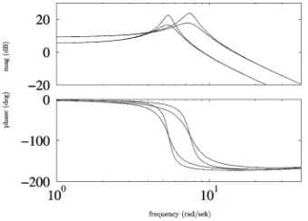
Fig. 7. Bode plots ofG (s)at the ends of the parameter intervals.
Fig. 8. Bode plots ofG (s)at the ends of the parameter intervals.
, for which Horowitz-Sidi bounds for 25 frequencies were computed. Algorithm 1 was then performed for both an controller (choosing the scaling factor ) and a PID controller with a second-order filter. was gradually increased up to 15 to reflect less strict constraints on the control signal, and the entire procedure was repeated for . All calculations were done with MATLAB on a 1-GHz Pentium III. Note that the number of constraints in the optimization
problem is for the design and
for the controller (one extra because of the constraint on the HF roll-off).
A. Discussion
For illustration, we present some details on the
de-sign case with and . The bounds on
the PID parameters were chosen to be
and .glcFast
[image:7.594.307.547.220.394.2]Fig. 9. Example (H ; G ; c = 1:5, andc = 1:5) of convergence of snopt. (a) Merit function versus iteration number. (b) Feasibility measure (dashed line) and optimality measure (solid line) versus iteration number.
[image:8.594.311.547.66.189.2](a) (b)
Fig. 10. LF performance(J )versus control activity(c )as obtained by Al-gorithm 1 for (a)G and (b)G with PIDf control (solid line) and PID weighted
H control (dashed line).
is feasible and optimal to within the specified tolerances of . was then increased to 2 and the optimal from the previous design was used as a starting point for snopt, without another global search. Convergence was achieved in four iterations (15 s).
[image:8.594.318.534.241.486.2]This can be compared to 10–20 min of computation in [15] and [16] to solve a smaller problem than here. Fig. 10 shows the results of the optimization in terms of obtained versus speci-fied and , and we note the general tradeoff between per-formance and control activity for all controllers. Thus, increased performance (reduced ) can be achieved without reducing the stability margin, but at a cost of higher control signals (increased ). Importantly for both plants, Algorithm 1 resulted in two sets of controllers ( and KPIDf) with equal values. This makes it easy to compare the two controller structures, because all closed loop properties that are not immediately compared are identically constrained. We see that the two controller structures perform similarly for both plants. This may be considered some-what surprising, since the controller is of order six for and ten for , compared to three for the KPIDf controller. Al-though the weighting function in the design is of PID type, the resulting sixth order controller is obviously more restricted than a lowpass filtered PID controller of third order. The reason
Fig. 11. Nyquist diagram forG with controllers optimized forc = 1:7 and c = 10. The five curves correspond to the cases [J d] =
[10 7:5]; [15 10]; [15 5]; [5 5]and[5 10].
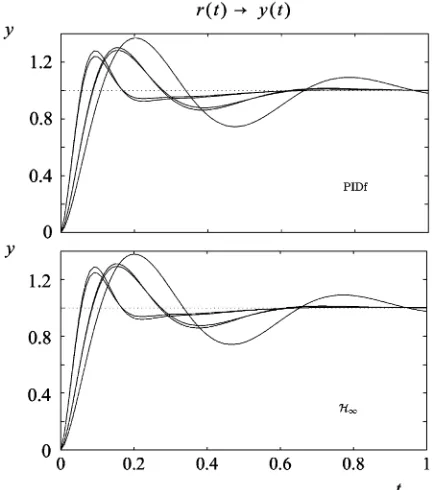
Fig. 12. Step responses from referencerto outputyforG with controllers optimized forc = 1:7andc = 10. The five curves correspond to the cases
[J d] = [10 7:5]; [15 10]; [15 5]; [5 5], and[5 10].
is that the parameters in the third order controller may take any value in the optimization of (13), while the design means that the stability robustness for a specific uncertainty model, re-lated to a normalized coprime factorization of the plant model, is optimized, cf. [21]. The benefit of SISO design is mainly for plants where an ordinary PID controller can be insufficient, for example, plants that are unstable, highly resonant, and non-minimum phase.
The algorithm resulted in nonconservative solutions for all specifications and in the sense that both
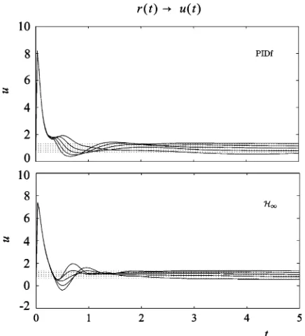
[image:8.594.45.280.268.426.2]Fig. 13. Step responses from referencerto control signaluforG with con-trollers optimized forc = 1:7andc = 10. The five curves correspond to the cases[J d] = [10 7:5]; [15 10]; [15 5]; [5 5], and[5 10].
Fig. 14. Nyquist diagram forG with controllers optimized forc = 1:7and
c = 10. The five curves correspond to the casesQ = 0:7; 0:85; 1:0; 1:15; and1:3.
1.0005 and 1.05, respectively. It was concluded that the smaller value improved by 1% and the larger value resulted in a 3% increase of . A smaller value of , however, implies a larger , which in turn results in deteriorating HF robustness prop-erties.
We also choose to study Nyquist plots and step responses for both plants from reference signal to output signal , and from reference signal to control signal , using the
con-trollers that result in and . Figs. 11–13
show these plots for with both the PID controller and the controller for the following values of the uncertain
pa-rameters: and .
Figs. 14–16 show the corresponding results for for the
flow rates: , and .
[image:9.594.319.537.361.601.2]The Nyquist plots verify that for both plants, indicating that the approximations made when defining the Horowitz-Sidi bounds were acceptable. The step responses indicate that the closed loop performance for the two controller
Fig. 15. Step responses from referencerto outputyforG with controllers optimized forc = 1:7andc = 10. The five curves correspond to the cases
Q = 0:7; 0:85; 1:0; 1:15;and1:3.
Fig. 16. Step responses from referencerto control signaluforG with con-trollers optimized forc = 1:7andc = 10. The five curves correspond to the casesQ = 0:7; 0:85; 1:0; 1:15;and1:3.
structures is practically identical for , and almost the same for , as indicated by the trade-off curves in Fig. 10.
VII. CONCLUSION
[image:9.594.46.287.365.489.2]to determine if the nominal open loop is (point wise) inside or outside the Horowitz–Sidi bounds in the Nichols chart.
The criteria used in the optimization procedure take into account important aspects for achieving robust control per-formance, including a guaranteed robustness to explicit plant uncertainties by use of Horowitz–Sidi bounds. Having separate criteria for the closed-loop properties in the different frequency regions facilitates the tradeoff between robustness and per-formance to be studied easily and clarifies the consequences of a change of specifications. The method also simplifies the task of comparing closed-loop performance between different controller structures, since closed loop properties in terms of stability robustness, control activity, and HF robustness are constrained identically.
The design method has been applied to two examples and it has been shown that a PID controller with a second-order filter on the derivative part achieves, more or less, the same low-frequency performance as an controller based on loop-shaping. Computationally, a substantial efficiency factor has been gained compared to an earlier, less general version of the design procedure.
REFERENCES
[1] B. Kristiansson and B. Lennartson, “Robust and optimal tuning of PI and PID controllers,” inIEE Proc. Control Theory Appl., 2002, vol. 149, no. 1, pp. 17–25.
[2] B. Lennartson and B. Kristiansson, “Pass band and high frequency ro-bustness for PID control,” inProc. 36th Conf. Decision Control, San Diego, CA, Dec. 1997, pp. 2666–2671.
[3] I. Horowitz, Quantitative Feedback Design Theory (QFT), D. D. Wagman, Ed. Boulder, CO: QFT Publications, 1993.
[4] P. O. Gutman, Qsyn, the Toolbox for Robust Control Systems Design for Use with Matlab [Online]. Available: www.math.kth.se/optsyst/re-search/5B5782/index.html 1996
[5] “MATLAB, Version 6, User’s Guide,”The Mathworks Inc., Natick, MA, 2000.
[6] G. F. Bryant and G. D. Halikias, “Optimal loop-shaping for systems with large parameter uncertainty via linear programming,”Int. J. Con-trol, vol. 62, no. 3, pp. 557–568, 1995.
[7] A. Gera and I. Horowitz, “Optimization of the loop transfer function,”
Int. J. Control, vol. 31, pp. 389–398, 1980.
[8] A. C. Zolotas and G. D. Halikias, “Optimal design of PID controllers using the QFT method,” inIEE Proc. Control Theory Appl., 1999, vol. 146, no. 6, pp. 585–589.
[9] G. D. Halikias, A. C. Zolotas, and R. Nandakumar, “Design of optimal robust fixed-structure controllers using the quantitative feedback theory approach,” inProc. Inst. Mech. Engineers Part I–J. Syst. Control Eng., 2007, vol. 221, pp. 697–716.
[10] O. Yaniv and M. Nagurka, “Design of PID controllers satisfying gain margin and sensitivity constraints on a set of plants,”Automatica, vol. 40, pp. 111–116, 2004.
[11] D. Garcia, A. Karimi, and R. Longchamps, “Robust proportional in-tegral derivative controller tuning with specifications on the infinity-norm of sensitivity functions,”IET Control Theory Appl., vol. 1, no. 1, pp. 263–272, 2007.
[12] S. Hara, T. Iwasaki, and D. Shiokata, “Robust PID control using gener-alized KYP synthesis—Direct open-loop shaping in multiple frequency ranges,”IEEE Control Syst. Mag., vol. 26, no. 1, pp. 80–91, Jan. 2006. [13] B. Kristiansson and B. Lennartson, “Simple and robust tuning of PI and PID controllers,”IEEE Control Syst. Mag., vol. 26, no. 1, pp. 55–69, Jan. 2006.
[14] B. Kristiansson and B. Lennartson, “Evaluation and simple tuning of PID controllers with high frequency robustness,”J. Process Control, vol. 16, no. 2, pp. 91–102, 2006.
[15] C. M. Fransson, B. Lennartson, T. Wik, and P. O. Gutman, “On op-timizing PID controllers for uncertain plants using Horowitz bounds,” inProc. IFAC Workshop Digital Control: Past, Present, and Future of PID Control, Terrassa, Spain, Apr. 2000, pp. 523–528.
[16] C. M. Fransson, B. Lennartson, T. Wik, and P. O. Gutman, “H con-trol for uncertain plants using Horowitz bounds,” inProc. Amer. Con-trol Conf., Arlington, VA, Jun. 2001, vol. 1–6, pp. 4103–4107. [17] C. M. Fransson, B. Lennartson, T. Wik, K. Holmström, M. A.
Saunders, and P. O. Gutman, “Global controller optimization using Horowitz bounds,” presented at the IFAC World Congress, Barcelona, Spain, Jul. 2002.
[18] C. M. Fransson, B. Lennartson, T. Wik, and K. Holmström, “Multi cri-teria controller design for uncertain MIMO systems using nonconvex global optimization,” inProc. 40th Conf. Decision Control, Orlando, FL, Dec. 2001, pp. 3976–3981.
[19] T. Wik, C. M. Fransson, and B. Lennartson, “Feedforward feedback controller design for uncertain systems,” inProc. 42nd Conf. Decision Control, Maui, HI, Dec. 2003, pp. 5328–5334.
[20] D. Galardini, M. Nordin, and P. O. Gutman, “Robust PI tuning for an elastic two-mass system,” presented at the Eur. Control Conf., Brussels, Belgium, Jul. 1997.
[21] D. McFarlane and K. Glover, “A loop shaping design procedure usingH synthesis,”IEEE Trans. Autom. Control, vol. 37, no. 6, pp. 759–769, Jun. 1992.
[22] J. Ackermann, Robust Control. Berlin, Germany: Springer-Verlag, 1993.
[23] P. O. Gutman, M. Nordin, and B. Cohen, “Recursive grid methods to compute value sets and Horowitz-Sidi bounds,”Int. J. Robust Non-linear Control, vol. 17, no. 2–3, pp. 155–171, 2007.
[24] P. O. Gutman, C. Baril, and L. Neumann, “An algorithm for computing value sets of uncertain transfer functions in factored real form,”IEEE Trans. Autom. Control, vol. 39, no. 6, pp. 1268–1273, Jun. 1994. [25] P. S. V. Nataraj and G. Sardar, “Template generation for continuous
transfer functions using interval analysis,”Automatica, vol. 36, pp. 111–119, 2000.
[26] D. R. Jones, The DIRECT Global Optimization Algorithm. Norwell, MA: Kluwer, 2001.
[27] P. E. Gill, W. Murray, and M. A. Saunders, “SNOPT: An SQP algo-rithm for large-scale constrained optimization,”SIAM J. Optimization, vol. 12, no. 4, pp. 979–1006, 2002.
[28] D. R. Jones, C. D. Perttunen, and B. E. Stuckman, “Lipschitzian opti-mization without the Lipschitz constant,”J. Optimization Theory Appl., vol. 79, no. 1, pp. 157–181, 1993.
[29] E. Galperin, “The cubic algorithm,”J. Math. Anal. Appl., vol. 112, pp. 635–640, 1985.
[30] J. Pinter, “Globally convergent methods for n-dimensional multiex-tremal optimization,”Optimization, vol. 17, pp. 187–202, 1986. [31] B. Schubert, “A sequential method seeking the global maximum of a
function,”SIAM J. Numer. Anal., vol. 9, pp. 379–388, 1972. [32] M. Björkman and K. Holmström, “Global optimization using the direct
algorithm in Matlab,”Adv. Modeling Optim., vol. 1, no. 2, pp. 17–37, 1990.
[33] M. Björkman and K. Holmström, “Global optimization of costly non-convex functions using radial basis functions,”Optim. Eng., vol. 1, no. 4, pp. 373–397, 2000.
[34] T. Hellström and K. Holmström, “Parameter tuning in trading algo-rithms using ASTA,” inComputational Finance 1999. Cambridge, MA: MIT Press, 1999.
Carl-Magnus Fransson, deceased, received the M.Sc. degree in chemical engineering with physics, the Lic. Eng. degree in control engineering, and the Ph.D. degree in automatic control from Chalmers University of Technology, Göteborg, Sweden, in 1999, 2001, and 2003, respectively.
Torsten Wikreceived the M.Sc. degree in chemical engineering in 1994, a Licentiate of Engineering degree in control engineering, the Ph.D. degree in environmental sciences, and the Docent degree from Chalmers University of Technology, Göteborg, Sweden, in 1994, 1996, 1999, and 2004, respectively. He is an Associate Professor with the Department of Signals and Systems, Chalmers University of Technology. From 2005 to 2007, he was a Senior Researcher with Volvo Technology AB where he was involved with control system development for engine test cells and for combined reformer and fuel cell systems. His current research interests are mainly in control issues related to model uncertainties, model simplification, process control, and environmental and microbiological applications.
Bengt Lennartsonreceived the M.Sc. degree in en-gineering physics and the Ph.D. degree in automatic control from Chalmers University of Technology (CTH), Göteborg, Sweden, in 1979 and 1986, respectively.
In 1989, he was an Associate Professor with the Control Engineering Laboratory, CTH, and in 1999, he was a Professor of the Chair of Automation, De-partment of Signals and Systems, CTH. He was Vice Dean of the School of Mechanical Engineering from 1998 to 2004 and Dean of Education at CTH from 2004 to 2007. He has also been Guest Professor with University West, Troll-hättan, Sweden, since 2005. His areas of interest include discrete event and hybrid systems as well as robust feedback control. He has been an Associate Editor forAutomaticaand a member of IFAC’s Technical Committee on Man-ufacturing. He is currently supervising 9 Ph.D. candidates, and he is the author or coauthor of 2 books and more than 150 peer-reviewed international papers.
Michael Saunderswas born in New Zealand and learned mathematics at the University of Canterbury, New Zealand. he received the Ph.D. degree in com-puter science from Stanford University, Stanford, CA, in 1972.
He specializes in numerical optimization and scientific computation. He is a core faculty member of SOL and iCME at Stanford University, where he teaches a graduate class on Large-scale Numerical Optimization. He is widely known for his contri-butions to mathematical algorithms and software, including the linear equation solvers SYMMLQ, MINRES, LSQR, LUSOL, LUMOD and the constrained optimization packages MINOS, LSSOL, NPSOL, QPOPT, SNOPT, SQOPT, and PDCO.
Prof. Saunders was elected Hon FRSNZ in 2007.
Per-Olof Gutman(SM’99) was born in Sweden, in 1949. He received the Ph.D. degree in automatic control from Lund Institute of Technology, Lund, Sweden, in 1982.