NASDAQ OMX OMS II Margin methodology guide for Equity and Index derivatives

NASDAQ OMX OMS II

Margin methodology guide for Equity and Index derivatives

7/31/2013

D

OCUMENT INFORMATION

Date Version Comments

2013-07-31 1.0 Initial

G

ENERAL READING GUIDELINES

The document is divided in two parts; a theoretical part that describes the basic principles and a practical part that contains margin calculation examples. In order to facilitate the reading, many of the mathematical explanations are found in the practical part of this document and in the appendix.

T

ABLE OF

C

ONTENTS

Document information ... 2

General reading guidelines ... 2

Background ... 5

Purpose of document ... 5

Introduction ... 6

margin requirement ... 6

Flows between NOMX and the clearing participants ... 6

1. OMS II Margin Methodology ... 8

Executive summary ... 8

Definitions ... 8

Liquidation Period ... 8

Valuation interval ... 8

Valuation points ... 8

Vector File/ Risk Matrix ... 9

Volatility shifts ... 9

Margin offset ... 9

Margin types ... 9

Parameters ... 10

Valuation interval ... 10

Pricing parameters ... 10

Window method (margin offset) ... 12

2. Margin calculations ... 13

Futures contracts ... 14

Example 1 – Index futures ... 14

Example 2 – Index futures at expiration ... 15

Forward contracts ... 15

Example 3 – Single stock forwards ... 16

Example 4 – Single stock forward at expiration ... 16

Options ... 17

Example 5 – Equity call option ... 19

Example 6 – Equity put option ... 20

Example 8 – Index option at expiry (Payment Margin) ... 21

Example 9 – Portfolio ... 22

Appendix I ... 24

Option valuation formulas ... 24

Binomial valuation model ... 24

Black-Scholes ... 25

Black-76 ... 26

Binary Options valuation ... 27

Window method ... 27

Window size ... 27

B

ACKGROUND

P

URPOSE OF DOCUMENT

The purpose of this document is to describe how margin calculations are performed and how the NASDAQ OMX’s OMS II margin methodology is applied for standardized equity and index derivatives.

I

NTRODUCTION

The margin requirement is a fundamental part of CCP clearing. In case of a clearing participant’s default, it is that participant’s margin requirement together with the financial resources of the CCP that ensures that all contracts registered for clearing will be honored.

 NOMX requires margins from all clearing participants and the margin requirement is calculated with the same risk parameters regardless of the clearing participant’s credit rating.

 The margin requirement shall cover the market risk of the positions in the clearing participant’s account. NOMX applies a 99.2% confidence level and assumes a liquidation period of two to five days (depending on the instrument) when determining the risk parameter.

F

NOMX

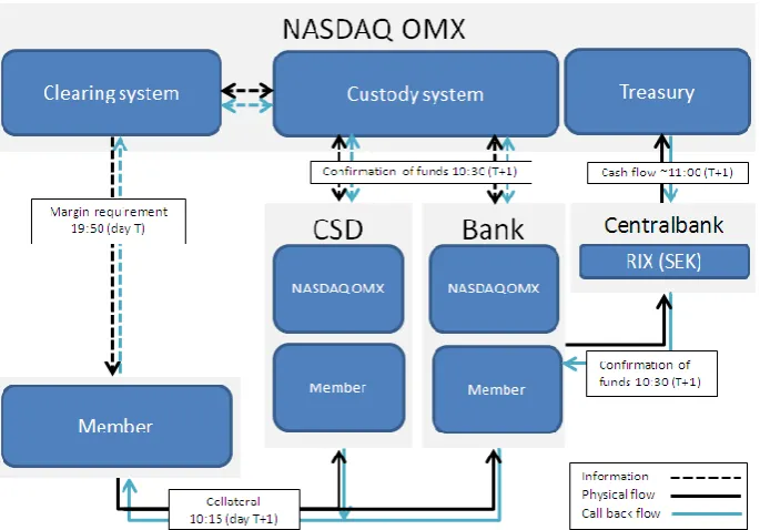
1. Margin – Collateral; NOMX calculates the margin requirement at the end of each trading day (T). The margin requirement becomes available to the clearing participants approximately at CET 20:00 on day T. The clearing participants have to cover their margin requirement with collateral. The clearing participants must have sufficient collateral in place before CET 10:30 on day T+1.

MA R GIN A N D SE T T L E M E N T F L O WS

Figure 1: Margin and call back flows.

1.

OMS

II

M

ARGIN

M

ETHODOLOGY

E

XECUTIVE SUMMARY

The NOMX OMS II margin methodology is a scenario based risk model that aims to produce a cost of closeout, given a worst case scenario. For OMS II, the scenarios are defined by the model’s input. The model inputs such as individual valuation intervals and volatility shifts are calculated with a minimum confidence level. OMS II is validated by back testing individual risk parameters and portfolio output. The confidence risk intervals are applied on each product using one year of historical price data.

To enable a trustworthy clearing service, reasonably conservative margins are required to avoid the risk of the clearing organization incurring a loss in a default. In theory, the margin requirement should equal the market value at the time of the default. However, under normal conditions an account cannot be closed at the instant a participant defaults at the prevailing market prices. It typically takes time to neutralize the account and the value of the portfolio can change during this period, which must be catered for in the margining calculation.

D

EFINITIONS

L

P

It can take time to neutralize a position and, as a result, a lead time exists from the moment collateral has been provided until the clearing organization is able to close the participant's portfolio. The length of the lead time depends on the time it takes to discover that the participant has not provided enough collateral and the time required to neutralize the portfolio.

V

OMS II varies the price for the underlying security for each series to calculate the neutralization cost. In this way, OMS II creates a valuation interval for each underlying security. The size of the valuation interval is given by the risk parameters for the instrument in question.

V

V

F

/

R

M

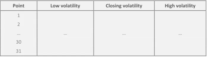
By adding position data to a risk matrix, we obtain the neutralizing cost in each valuation point for a single position. The risk matrix is a vector file in which each cell is a valuation point. In one dimension the underlying price is altered and in the other the volatility is altered. If this instrument is not affected by volatility, i.e. futures and forwards, the values for the different volatilities will be the same. Different vector files are created for bought and sold positions.

Figure 2: Example of a vector file

Point Low volatility Closing volatility High volatility

1 2

… … … …

30 31

V

The price of an option can be strongly affected by changes in volatility. The risk of fluctuations in volatility is taken into account by calculating the value of the account, based not only on the current volatility, but also on a higher and a lower volatility. The amount by which the volatility is increased or decreased is determined and configured by NOMX. The neutralizing cost is calculated at each of the valuation points for three different volatility levels; hence for options a valuation interval consists of 3 X 31 valuation points.

M

In case price dependencies are observed, NOMX can provide offsets in margins between different instruments within the same instrument group as well as offsets between different instruments from different instrument groups. Margin offset is only provided in case correlation between products historically has been high and proven stable. In the OMS II model the margin offsets are calculated by portfolio. Offsets are provided when the shift (stress) of the underlying prices of the products demonstrate a stable dependency. For options, the deviation in the shift (stress) of the implied volatilities is also assessed to decide the offset level.

Currently OMS II only apply offset for contracts with the same underlying instrument.

M

NA K E D M A RG IN

A position’s margin requirement shall cover future market movements. The margin requirement is calculated using vector files. The naked margin is the margin requirement of a portfolio/position where no cross margining is applied.

PA Y M E N T M A RGIN

margin is applied to cover the risk of a participant failing to fulfill the settlement payment.

DE L IVE RY M A RGIN

A position’s delivery margin consists of the position’s profit and loss plus the position’s scenario risk. Delivery margin is required for all stock products and is applied between expiration and settlement.

P

ARAMETERS

This section covers the configurable parameters utilized in the margin calculations for forwards, futures and options.

OMS II uses theoretical formulas for pricing options in each valuation point. The valuation formula differs depending on the option type. The specific valuation formula for each option type is specified in the appendix.

V

Parameter Description

Risk parameter Determines the size of the valuation interval. The parameter is a percentage of the underlying price.

P

Parameter Description

Risk free interest rate (%) Risk-free interest rate used when evaluating options. The simple interest rate is translated to a continuous rate.

Dividend yield (%) Dividend yield used when evaluating options. To properly evaluate American options on futures, the dividend yield is set equal to the risk free interest rate.

Adjustment for erosion of time value

The number by which the number of days to maturity will be reduced when evaluating held options.

Adjustment of futures (%) Adjustment factor (spread parameter) for futures.

Highest volatility for bought options

Applies only to bought options.

Lowest volatility for sold options Applies only to sold options.

Volatility shift parameter Fixed parameter that determines the size of the volatility interval.

Volatility spread Defines the spread for options. The spread parameter is a fixed value.

Highest value bought in relation to sold options (%)

Min. spread between the values for bought and sold options; if spread is too small the value of the bought option is decreased.

Adjustment for negative time value

Adjustment for negative time value

If the theoretical option value is lower than the intrinsic value, the price is adjusted to equal the latter.

Underlying price The price of the underlying (stock or index etc.) in

this valuation point.

Strike price The strike price of the option.

Volatility See the following section.

Time to expiration of the option Calculated as number of actual days / risk parameter. Days Per Year For Interest Rate Calculations.

Dividends Known or expected dividends of the underlying

affects the value of the option. This can be modeled as a continuous dividend yield or with discrete dividends (time and amounts).

VO L A T IL IT Y

NOMX uses the implied volatility which is based on the price of the individual option. Two separate volatilities are calculated, one for bought and one for sold options. The volatility for bought options is based on the bid price of the option, and the volatility for sold options is based on the ask price of the option.

When calculating implied volatility for exchange traded options, there are two opposing forces to consider: flexibility and stability. Using the individual implied volatility for each series theoretically allows the clearing organization to cover smile effects in volatility. However, the problem with obtaining accurate pricing for less liquid instruments makes this method unstable in such case.

To account for smile effects, NOMX applies a volatility surfaces model1 for the most liquid instruments. For other liquid instruments, an arithmetic average is calculated for the three closest at-the-money series for each expiration and underlying instrument. The mean value is then used as market volatility. For the most illiquid instruments NOMX applies a fixed volatility. The two latter methods do not consider smile effects, but have proven to be very stable.

FIN E T UN IN G

In order to obtain more appropriate margin requirements the following fine tuning features are used by OMS II. These features are illustrated in the following sections.

Adjustment for erosion of time

In the case of bought options, the clearing house will have to sell the position in a default situation. This means that the clearing house will probably have to sell an option with a shorter time to delivery because of the lead time. This motivates that the time to expiration used when valuating bought positions is reduced by the number of lead days.

Min/max volatility

In order not to value bought options too high, the volatility used for bought options has a maximum value. The value is defined in the risk parameter Highest Volatility

1

for bought Options. A similar approach is used for sold positions where the volatility is not allowed to go below a minimum value.

Negative time value

A bought option is adjusted for negative time value if the volatility is zero. Since this would indicate a negative time value, the following factor is calculated:

If this factor is less than 1, the factor is later multiplied to all the bought option values in the vector file. In this way, the theoretical values are scaled to give a better representation of the market. This adjustment is only made for bought positions. The most common case when this occurs is when projected dividends are not used in the margin calculations.

Minimum value sold options

For a sold option with a theoretical value of less than 0.01 NOMX apply a minimum value of 0.01.

Minimum spread bought/sold options

The spread between bought and sold options is not allowed to become too narrow. This is prevented by comparing vector file values for bought and sold options in the same valuation point and adjusting the value of the bought option if needed. The current spread is set to 95% for a bought option in relation to a sold option.

Rounding

As a last step, the vector file values are multiplied by the contract size and then rounded to two decimal places. In the subsequent equations means rounding to two decimals.

W

(

)

For different instruments that show a high correlation to each other, there is a need for a method that takes this into consideration with respect to margining calculations. The method used in the OMS II methodology is called the “window method”. In this method, the scanning range limits the individual movement for each series, but there is a maximum allowed difference between the scanning points of the two series. This range can be represented as a window, hence the name. The size of this window is estimated roughly by the same method that is used to estimate scanning ranges. Daily differences between the movements of the series are calculated using one year of data. These values are then used to build a numerical cumulative distribution from which 99.2 % confidence interval is applied.

Based on a given covariance, the window can display a spread demonstrating the maximum allowable difference in price variation between two different underlying securities. In a narrow window, prices cannot vary as much as in a broad one. As a result, high covariance causes a narrow window, and vice versa.

2.

M

ARGIN CALCULATIONS

In the subsequent sections margin calculations for futures, forwards and options are illustrated.

DE F IN IT IO N S

Variable Definition

RMB Required margin for bought contracts

RMS Required margin for sold contracts

DLV Delivery margin

P Spot price of underlying stock/Index value

Ft Fixing price (Margin settlement price) of future/forward on day t

CP Contract price

Q Number of contracts

T Time to expiration day expressed in years (days/365)

VOLAP Volatility used for a sold put option (based on ask prices)

VOLBP Volatility used for a bought put option (based on bid prices)

VOLAC Volatility used for a sold call option (based on ask prices)

VOLBC Volatility used for a bought call option (based on bid prices)

Instrument data

CS Contract size. The number of instruments that defines one contract for

an instrument

S Strike price of the option

DIVI

Discrete dividend number that is included in the valuation of the option. Offset days for dividends If the value equals 0, this is dividends with ex-date in the time range ( current ex-date + 1 : expiration ex-date). If the value equals 1, this is dividends with ex-date in the time range ( current date + 1 : expiration date + 1 )

Risk parameters

Par Risk interval parameter (variable)

Vu/d

Volatility shift parameter i.e. the maximum increase/ decrease in volatility

AD Adjustment factor (spread)

r Risk free interest rate

q Dividend yield

ER Adjustment for erosion of time value

In the following equations means rounding to two decimals.

F

UTURES CONTRACTS

Bought position

1

Sold position:

2

PA Y M E N T M A RGIN

Bought position

3

Sold position:

4

E

1

–

I

PO SIT IO N

Consider a position of 50 bought OMXS303A contracts expiring in January 2013.

PA RA M E T E RS A N D VA RIA B L E S

Ft 926.48

P 927.47

Par 8.5%

AD 0.5%

Q 50

CS 100

MA R GIN CA L CUL A T IO N

Using equation 1:

E

2

–

I

PO SIT IO N

100 sold OMXS30 futures contracts expiring today.

PA RA M E T E RS A N D VA RIA B L E S

Ft 952.50

Ft-1 950.00

Q 100

CS 100

MA R GIN CA L CUL A T IO N (PA Y M E N T M A RGIN)

Using equation 4:

Payment margin on futures contracts is only used at expiration. The margin requirement equals the final cash settlement amount of the contract.

F

ORWARD CONTRACTS

Bought position

)

)

5

Sold position

)

6

DE L IVE RY M A RGIN

Bought position

)

)

7

Sold position

E

3

–

S

PO SIT IO N

100 sold HMB forward contracts with expiry in December 2013.

PA RA M E T E RS A N D VA RIA B L E S

Ft 245.89

P 243.80

CP 295,70

Par 7.5%

AD 2%

Q 100

CS 100

MA R GIN CA L CUL A T IO N

Using equation 6:

)

)

)

The worst case value of this position is found at the top of the vector file, i.e. the price of the forward increases.

E

4

–

S

PO SIT IO N

100 bought HMB forwards expiring today.

PA RA M E T E RS A N D VA RIA B L E S

P 410.00

CP 390.00

Par 10%

AD 2%

Q 100

CS 100

MA R GIN CA L CUL A T IO N (DE L IVE RY M A R GIN)

Using equation 7:

)

)

)

)

O

PTIONS

The option price as a function of the underlying price is non-linear. Genium Risk assumes that two major factors affect option prices:

 Underlying price  Implied volatility

For a position consisting of one option, we know that the largest and smallest option value will be at the end points of the interval. E.g. a bought (sold) call will have the smallest value when underlying stock price and volatility are as low (high) as possible.

NA K E D M A RG IN F O R E Q UI T Y O PT IO N S

Equity options are defined as premium paid options with American style expiry.

Bought call option

]

9

Bought put option

]

10

Sold call option

[

]

11

Sold put option

[

]

12

DE L IVE RY A N D SE T T L E M E N T F O R E Q UIT Y O PT IO N S

If the options are to be exercised, the delivery margin at exercise is calculated in the following manner:

Bought call option sold Put option or

)

13

Sold call option or Bought put option

NA K E D M A RG IN F O R IN DE X O PT IO N S

Standardized index options are European future style options where the margin requirement is calculated similarly to premium paid options.

Bought call option

]

15

Bought put option

]

16

Sold call option

]

17

Sold put option

]

18

DE L IVE RY A N D SE T T L E M E N T F O R IN DE X O PT IO N S

For cash settled options, for example index options, there is no market risk between exercise and delivery (IV is the index value at exercise).

Exercise (the seller has to pay)

19

20

Delivery (the seller has to pay)

21

E

5

–

E

Consider a position with 10 sold Call options with 32 days to expiry.

PA RA M E T E RS A N D VA RIA B L E S

S 220.00

P 237.20

DIV none

r 3%

P 10

Par 7.5%

AD 2%

VU 10

CS 100

Q 10

T 32/365

VOLAC 18.85%

For each scenario point using equation 10:

[ ]

The vector file combines the price- and volatility scenarios:

VE CT O R F IL E

Scenario Vol Down Vol Mid Vol Up

1 -35 380 -35 390 -35 700

2 -34 190 -34 200 -34 570

3 -33 000 -33 030 -33 430

4 -31 820 -31 850 -32 300

5 -30 630 -30 670 -31 160

6 -29 450 -29 490 -30 030

7 -28 260 -28 320 -28 950

8 -27 070 -27 160 -27 870

9 -25 890 -26 000 -26 800

10 -24 700 -24 830 -25 720

11 -23 520 -23 680 -24 640

12 -22 330 -22 550 -23 560

13 -21 140 -21 410 -22 540

14 -19 960 -20 280 -21 550

15 -18 770 -19 160 -20 560

16 -17 590 -18 080 -19 570

17 -16 400 -17 000 -18 570

18 -15 220 -15 920 -17 580

19 -14 040 -14 860 -16 650

20 -12 870 -13 870 -15 780

21 -11 710 -12 880 -14 920

23 -9 420 -10 930 -13 190

24 -8 320 -10 060 -12 320

25 -7 240 -9 200 -11 520

26 -6 240 -8 340 -10 810

27 -5 250 -7 520 -10 100

28 -4 380 -6 820 -9 390

29 -3 550 -6 110 -8 690

30 -2 840 -5 400 -7 980

31 -2 210 -4 780 -7 350

MA R GIN RE Q U IRE M E N T

The worst case scenario for a sold call position is to stress the price and volatility up. Hence the margin requirement for this position is:

E

6

–

E

Consider a sold put option position.

PA RA M E T E RS A N D VA RIA B L E S

S 230.00

P 237.20

DIV None

r 3%

Par 7.5%

AD 2%

VU 10

CS 100

Q 1

T 32/365

VOLAP 17.79%

MA R GIN CA L CUL A T IO N

Using equation 11:

[

]

MA R GIN RE Q U IRE M E N T

By combining each scenario point for price and volatility we create the vector file. The worst-case value for a sold put option is to stress the price down and the volatility up. Thus we will find the margin requirement in the bottom right corner of the vector file.

E

7

–

E

(D

M

)

Consider a portfolio consisting of 50 sold contracts.

PA RA M E T E RS A N D VA RIA B L E S

S 36

P 18

DIV None

r 3%

Par 25%

AD 2%

VU 10

CM 100

T 32/365

Q 50

VOLAP 17.79%

MA R GIN CA L CUL A T IO N

Using equation 13:

)

MA R GIN RE Q U IRE M E N T

Thus the delivery margin for the position is:

E

8

–

I

(P

M

)

Consider a cash settled European call option at expiration, payment margin.

PA RA M E T E RS A N D VA RIA B L E S

S 1000

IV 922

Q 10

CS 100

MA R GIN CA L CUL A T IO N (PA Y M E N T M A RGIN)

Using equation 19:

MA R GIN RE Q U IRE M E N T

E

9

–

P

Consider a portfolio consisting of 50 bought OMXS30 futures contracts and 70 sold OMXS30 options expiring in January 2013. To calculate the margin requirement of this portfolio the window method is used. The window size in this example is 0%, which corresponds to 100% correlation.

VE CT O R F IL E S

50 bought OMXS303A futures

70 sold OMXS303A920 call options

Point Ft Point Ft Vol = 14.42% Vol = 24.42% Vol = 34.42%

1 1005.31 371 000 1 1005.31 -621 110 -708 120 -819 490

2 1000.06 344 750 2 1000.06 -588 490 -679 560 -793 030

3 994.80 318 450 3 994.80 -556 430 -651 560 -766 990

4 989.55 292 200 4 989.55 -524 860 -624 050 -741 370

5 984.29 265 900 5 984.29 -493 990 -597 030 -716 100

6 979.04 239 600 6 979.04 -463 750 -570 500 -691 250

7 973.78 213 350 7 973.78 -434 210 -544 530 -666 820

… … … …

25 879.18 -259 650 25 879.18 -73 290 -185 150 -304 570

26 873.92 -285 950 26 873.92 -63 630 -171 570 -289 030

27 868.67 -312 200 27 868.67 -54 950 -158 690 -273 980

28 863.41 -338 500 28 863.41 -47 110 -146 510 -259 490

29 858.16 -364 800 29 858.16 -40 250 -134 960 -245 420

30 852.90 -391 050 30 852.90 -34 090 -124 040 -231 910

31 847.65 -417 350 31 847.65 -28 770 -113 750 -218 820

As seen in the vector files the two individual worst case values are located on opposite sides in the valuation interval. These values are referred to as each position’s naked margin requirement. If there was no correlation between the instruments the portfolio’s total margin requirement would equal the sum of these values. A window is applied to determine the maximum allowable difference in price variation. In this case, the window size is 0% which corresponds to a window that is 1 row wide. The number of rows used in the window method is determined by the following set of calculations:

1. Let x = (1.0 – window size/100)*(# points – 1) x = (1 – 0/100) * (31 – 1) = 30

2. Round x to nearest integer x = 30

3. Let x = # points – x x = 31 – 30 = 1

SL ID IN G W IN DO W

50 bought OMXS303A futures 70 sold OMXS303A920 call options

1 371 000 371 000 371 000 -621 110 -708 120 -819 490

2 344 750 344 750 344 750 -588 490 -679 560 -793 030

3 318 450 318 450 318 450 -556 430 -651 560 -766 990

4 292 200 292 200 292 200 -524 860 -624 050 -741 370

5 265 900 265 900 265 900 -493 990 -597 030 -716 100

6 239 600 239 600 239 600 -463 750 -570 500 -691 250

7 213 350 213 350 213 350 -434 210 -544 530 -666 820

… … … … …

25 -259 650 -259 650 -259 650 -73 290 -185 150 -304 570

26 -285 950 -285 950 -285 950 -63 630 -171 570 -289 030

27 -312 200 -312 200 -312 200 -54 950 -158 690 -273 980

28 -338 500 -338 500 -338 500 -47 110 -146 510 -259 490

29 -364 800 -364 800 -364 800 -40 250 -134 960 -245 420

30 -391 050 -391 050 -391 050 -34 090 -124 040 -231 910

31 -417 350 -417 350 -417 350 -28 770 -113 750 -218 820

In the example above the sliding window is centered over row 7. The worst case value in this window is 213 350 + (-666 820) = -453 470. The overall worst case value, and the total margin requirement of the portfolio, is found at the bottom of the vector file, and equals -636 170.

SUM M A T RIX

Sum matrix

1 -250 110 -337 120 -448 490

2 -243 740 -334 810 -448 280

3 -237 980 -333 110 -448 540

4 -232 660 -331 850 -449 170

5 -228 090 -331 130 -450 200

6 -224 150 -330 900 -451 650

7 -220 860 -331 180 -453 470

… … … …

25 -332 940 -444 800 -564 220

26 -349 580 -457 520 -574 980

27 -367 150 -470 890 -586 180

28 -385 610 -485 010 -597 990

29 -405 050 -499 760 -610 220

30 -425 140 -515 090 -622 960

31 -446 120 -531 100 -636 170

As the window slides down the vector files, worst case values are calculated at each point. The naked margin for each contract is found within the window where the overall worst case value is found. The sum of each position’s naked margin equals the total margin requirement.

MA R GIN RE Q U IRE M E N T

Series Bought Sold Naked margin Margin

OMXS300A 50 -417 350 -417 350

OMXS300A920 70 -819 490 -218 820

A

PPENDIX

I

O

PTION VALUATION FORMULAS

The following table shows the various NOMX uses for options with and without dividends. The risk free interest rate is denoted r and the dividend yield is denoted as q.

Product Method without dividends Method with discrete dividends

American call based on spot Black -Scholes Binomial with dividends

American put based on spot Binomial if interest rate is non-zero, Black -Scholes if interest rate equals zero.

Binomial with dividends

European opt based on spot Black -Scholes Discount spot with dividends,

then use Black -Scholes

European opt based on future

Black -76 Black -76

Binary Cash-or-Nothing based on spot

Standard formula Discount spot with dividends,

then use Black -Scholes

Binary Cash-or-Nothing based on future

Standard formula with q = r Standard formula with q = r

Below sections illustrate the option valuation formulas used by NOMX. These are well known, widely used industry-standard formulas which can be found in the financial literature e.g. Hull 2011.

B

The binomial pricing model traces the evolution of the option's underlying variables in time. This is done by means of a binomial tree, for a number of time steps between the valuation and expiration dates. NOMX utilize a tree structure with 30 steps. The following values for the parameters in the method are used:

DE F IN IT IO N S

Variable Definition

C Call price

P Put price

S0 Stock price at time zero

K Strike price

r Continuously compounded risk-free rate

Q Dividend yield

σ Stock price volatility

u Up movement

d Down movement

p Probability up movement

1-p Probability down movement

Up movement:

) √

)

Down movement:

Probability:

where

and

₎

The discounting when walking backwards in the tree is done with r (not r-q).

Black-Scholes

The Black-Scholes formula calculates the price of European put and call options.

DE F IN IT IO N S

Variable Definition

C Call price

P Put price

S0 Stock price at time zero

K Strike price

r Continuously compounded risk-free rate

σ Futures price volatility

T Option’s time to maturity

)

₎

And

₎

₎

(

_{) (}

₎

√

and

(

_{) (}

₎

√

√

The function N(x) is the cumulative distribution function for a standardized normal distribution.

B

-76

For options on futures contracts the Black-76 formula is used.

DE F IN IT IO N S

Variable Definition

C Call price

P Put price

F0 Futures price at time zero

K Strike price

r Continuously compounded risk-free rate

σ Stock price volatility

T Option’s time to maturity

₎

₎₎

and

₎

₎₎

Where

(

_{) (}

₎

√

and

(

_{) (}

₎

B

O

For binary Cash-or-Nothing options the definitions follow the Black-Sholes notation.

DE F IN IT IO N S

Variable Definition

C Call price

P Put price

S0 Stock price at time zero

K Strike price

Q Fixed payout amount

r Continuously compounded risk-free rate

σ Stock price volatility

T Option’s time to maturity

Cash-or-nothing call option:

₎

Cash-or-nothing put option:

₎

W

INDOW METHOD

Generally the default cross margining may be described as instruments with the same underlying being totally correlated, and instruments with different underlying instruments being non-correlated.

However, a more advanced correlation method, called the window method, can be utilized. In this method, the different instruments are sorted into a number of groups called window classes. Each window class has a window size in percent. Price correlation goes up when the window size goes down. A window size of 0% means full price correlation and a window size of 100% means no price correlation. Additionally, each window class may, or may not, use volatility correlation.

A window class may also be a member of another window class, thereby creating a tree-structure in order to achieve more complicated correlations.

W

The window size (WS) roughly corresponds to the inverse of the correlation of two or more instruments. To determine the correlation between instruments, the window size is calculated by using the instruments’ normalized daily price changes in percentage. Based on one year of historical data the second largest difference is chosen.

1. Price changes in percentage per underlying instrument (i=1 to n) over a time period (t=1 to T).

∑

)

∑

)

3. A vector containing the largest price difference between instruments for each t is calculated.

∑ ) )

4. The second largest value from the vector is obtained

∑ ) )

)

The obtained parameter, that is the maximum allowable price difference, is the risk interval parameter. Since the size of the risk interval is twice as big as the parameter (both up and down price stress is implied) the parameter needs to be divided by 22

5. The parameter is then multiplied by liquidation period hence the Window Size equals:

∑ ) ) ) √

N

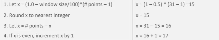
The algorithm for converting a window size in percent into points is shown below.

Figure 3: Algorithm for converting window size to valuation point

1. Let x = (1.0 – window size/100)*(# points – 1) x = (1 – 0.5) * (31 – 1) =15

2. Round x to nearest integer x = 15

3. Let x = # points – x x = 31 – 15 = 16

4. If x is even, increment x by 1 x = 16 + 1 = 17

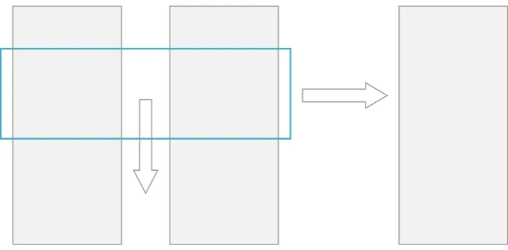
The sum matrix values the combined position in each valuation point. The margin requirement will equal the sum of the worst case from each individual position within the sliding window.

2

Figure 4: Illustration of the window method, where X and Y are individual worst case values