https://doi.org/10.5194/angeo-36-761-2018 © Author(s) 2018. This work is distributed under the Creative Commons Attribution 4.0 License.
Comparison of accelerometer data calibration methods used in
thermospheric neutral density estimation
Kristin Vielberg1, Ehsan Forootan1,2, Christina Lück1, Anno Löcher1, Jürgen Kusche1, and Klaus Börger3
1Institute of Geodesy and Geoinformation, University of Bonn, Nussallee 17, 53115 Bonn, Germany 2School of Earth and Ocean Sciences, Cardiff University, Cardiff CF10 3AT, UK
3German Space Situational Awareness Centre (GSSAC), Mühlenstrasse 89, 47589 Uedem, Germany
Correspondence:Kristin Vielberg ([email protected])
Received: 24 November 2017 – Revised: 24 April 2018 – Accepted: 2 May 2018 – Published: 18 May 2018
Abstract. Ultra-sensitive space-borne accelerometers on board of low Earth orbit (LEO) satellites are used to mea-sure non-gravitational forces acting on the surface of these satellites. These forces consist of the Earth radiation pres-sure, the solar radiation pressure and the atmospheric drag, where the first two are caused by the radiation emitted from the Earth and the Sun, respectively, and the latter is related to the thermospheric density. On-board accelerometer mea-surements contain systematic errors, which need to be mit-igated by applying a calibration before their use in grav-ity recovery or thermospheric neutral densgrav-ity estimations. Therefore, we improve, apply and compare three calibra-tion procedures: (1) a multi-step numerical estimacalibra-tion ap-proach, which is based on the numerical differentiation of the kinematic orbits of LEO satellites; (2) a calibration of accelerometer observations within the dynamic precise orbit determination procedure and (3) a comparison of observed to modeled forces acting on the surface of LEO satellites. Here, accelerometer measurements obtained by the Gravity Recovery And Climate Experiment (GRACE) are used. Time series of bias and scale factor derived from the three cal-ibration procedures are found to be different in timescales of a few days to months. Results are more similar (statisti-cally significant) when considering longer timescales, from which the results of approach (1) and (2) show better agree-ment to those of approach (3) during medium and high solar activity. Calibrated accelerometer observations are then ap-plied to estimate thermospheric neutral densities. Differences between accelerometer-based density estimations and those from empirical neutral density models, e.g., NRLMSISE-00, are observed to be significant during quiet periods, on av-erage 22 % of the simulated densities (during low solar
ac-tivity), and up to 28 % during high solar activity. Therefore, daily corrections are estimated for neutral densities derived from NRLMSISE-00. Our results indicate that these correc-tions improve model-based density simulacorrec-tions in order to provide density estimates at locations outside the vicinity of the GRACE satellites, in particular during the period of high solar/magnetic activity, e.g., during the St. Patrick’s Day storm on 17 March 2015.
Keywords. Atmospheric composition and structure (instru-ments and techniques)
1 Introduction
Recent gravimetric satellites, for example the satellite mis-sions CHAllenging Minisatellite Payload (CHAMP; Reig-ber et al., 2002) or Gravity Recovery And Climate Experi-ment (GRACE; Tapley et al., 2004), are equipped with ultra-sensitive space-borne accelerometers that allow for the mea-surement of non-gravitational forces acting on the surface of these satellites. These measurements reflect accelerations due to the atmospheric drag (the dominant component of the acceleration vector at the orbital altitude of these satellites), and thus enable studies of thermospheric neutral density and winds (e.g., Bruinsma et al., 2004; Liu et al., 2005; Sutton et al., 2007; Doornbos, 2012; Lei et al., 2012; Mehta et al., 2017). Non-gravitational forces also contain the effect of the solar and Earth radiation.
deter-mination (e.g., Van Helleputte et al., 2009). This is mainly because of systematic errors that contaminate the sensor data. Calibrating the ultra-sensitive space-borne accelerome-ters before the satellite’s launch is not possible, since gravity on the Earth’s surface is too large and simulating the space environment is extremely difficult. Therefore, several stud-ies have been developed during the last decade to ensure in-orbit calibration of accelerometer measurements. For exam-ple, Kim (2000), Tapley et al. (2004) and Klinger and Mayer-Gürr (2016) calibrate GRACE accelerometer observations within a gravity field recovery procedure. Bezdˇek (2010) and Calabia et al. (2015) apply numerical differentiation tech-niques, e.g., developed by Reubelt et al. (2003), to compute accelerations from precise kinematic orbits, which are then used to estimate calibration parameters and their uncertain-ties. Alternatively, calibration parameters can be estimated within the precise orbit determination procedure (Bettadpur, 2009; Van Helleputte et al., 2009; Visser and Van den IJssel, 2016). Each method mentioned above yields different cali-bration parameters and their uncertainty, and their influence on the final products such as thermospheric neutral density estimation has not yet been systematically investigated.
In order to better understand and reconcile differing results in the literature, three calibration procedures are applied to GRACE accelerometer measurements in this study. The aim is to assess the impact of a specific calibration method on the estimation of global thermospheric neutral densities as will be discussed in what follows. (1) The first approach is here called the multi-step numerical estimation (MNE), which is based on the numerical differentiation of kinematic positions. The application of this method is similar to that of Bezdˇek (2010) with few differences concerning the orbit data and the stage in which calibration parameters are estimated. (2) The second approach calibrates GRACE accelerometer measure-ments within the dynamic precise orbit determination proce-dure (Löcher, 2011). (3) Finally, calibration parameters are obtained by comparing the accelerometer measurements to modeled non-gravitational forces acting on the satellite. This procedure is commonly used to find initial calibration pa-rameters in gravity recovery experiments (e.g., Kim, 2000; Van Helleputte et al., 2009; Klinger and Mayer-Gürr, 2016). In recent decades, empirical and physical models of the atmosphere have gone through considerable development, while reflecting the range of density variability in response to solar and geomagnetic forcing. The Mass Spectrome-ter and Incoherent ScatSpectrome-ter (MSIS) empirical models of the neutral atmosphere (Picone et al., 2002) have been devel-oped since 1977. Other models such as the Jacchia–Bowman (e.g., Bowman et al., 2008) have also been used in vari-ous satellite applications. The current models NRLMSISE-00 and Jacchia–Bowman 2NRLMSISE-008 are built from an extensive drag data set and they are parameterized in terms of solar and magnetic indices at daily and 3-hourly resolution, re-spectively. In this study, we show to what extent GRACE-derived calibrated accelerometer data affect the final
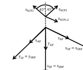
esti-Figure 1.Satellite body fixed reference frames (modified from Bet-tadpur, 2012). Here, SRF represents the science reference frame, AF and SF respectively stand for the accelerometer frame and the satellite frame and SCF indicates the star camera frame.
mation of atmospheric neutral density. Furthermore, as em-pirical thermospheric models fall short of simulating ther-mospheric neutral density (mostly at short timescales and during high solar/magnetic activity, Bruinsma et al., 2004; Guo et al., 2007), daily empirical corrections are estimated, which can be applied to scale the outputs of these models, and therefore improve their global performance particularly during high geomagnetic activity (see Sect. 4.3).
In the following, data sets and models are introduced in Sect. 2, and the methodologies of calibration are discussed in Sect. 3. The results are presented in Sect. 4 and the study is concluded in Sect. 5.
2 Data
2.1 GRACE data
We use GRACE Level-1B data (Case et al., 2010)1provided in the science reference frame (SRF) located at the center of mass of each satellite. The axes of the SRF are parallel to the accelerometer frame (AF) and the satellite frame (SF, see Fig. 1). Following this, the x axis points to the phase center of the K-Band instrument (along-track or anti-along-track direction depending on leading or trailing satellite), the
zaxis is directed to the normal of thex axis and the main equipment platform plane. They axis completes the right-handed triad.
2.1.1 Accelerometer
Space-borne capacitive accelerometers such as the Super-STAR accelerometer on board each GRACE twin satellites contain a proof mass, which is kept at the center of mass of a satellite by compensating the non-gravitational forces with
1ftp://podaac-ftp.jpl.nasa.gov/allData/grace/L1B/JPL/RL02/;
[image:2.612.334.507.65.211.2]induced electrostatic forces. The measured accelerations of the proof mass of the SuperSTAR accelerometer, which are proportional to the voltage needed to generate the compen-sating electrostatic forces, are labeled as ACC1B within the GRACE Level-1B data.
This accelerometer has a resolution of 10−10m s−2in the
x and zdirections, whereas the resolution of they axis is found to be one magnitude lower (Flury et al., 2008). The temporal resolution of the ACC1B data is 1 s. Frommknecht (2007) showed that the noise level of the along-track and radial components of the accelerometer is 2–3 times higher than that specified in the handbook. However, the noise level is reported to be similar for both satellites. Possible reasons for systematic effects are axis non-orthogonality, displace-ment of the test mass with respect to the satellite’s center of mass and thermal effects (Frommknecht, 2007).
2.1.2 Star camera
Two star cameras on board each GRACE satellite provide its inertial orientation in terms of quaternions, labeled as SCA1B. These data are used (in Sect. 3.1) to transform mea-surements given in the SRF to the celestial reference frame (CRF).
2.1.3 Macro model
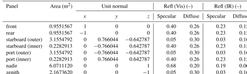
In this study, a macro model is required to model the non-gravitational accelerations acting on the surface of the satel-lite (Sect. 3.3). The geometry of the two identical GRACE satellites is represented in a macro model (Bettadpur, 2012) including mass, surface area and material of each plane in terms of visible and infrared reflectivity coefficients for spec-ular and diffuse reflection (see Table 1). The characteristics of the macro model have been determined under laboratory conditions; their values may be different under space con-ditions. These values also change during the mission’s life-time due to aging of the surface coating under UV radiation (Vallado and Finkleman, 2014). Following this, we make use of the macro model at hand, and an estimation of their un-certainty, as well as their impacts on the final thermospheric density estimations will be addressed in another study. 2.2 Precise orbits
Each GRACE satellite is equipped with three GPS receivers, whose data are used for precise orbit determination (POD) and which ensure the precise time tagging of other on-board measurements. Level-1B GRACE satellite orbits (GNV1B) are obtained from a dynamic POD procedure (Case et al., 2010). However, the choice of orbit data depends on their application. Since here we aim at calibrating accelerome-ter measurements for thermospheric density estimations, the kinematic precise orbits, which are free from accelerometer measurements, are applied. For this, kinematic orbits are
pro-cessed by the Graz University of Technology (Zehentner and Mayer-Gürr, 2016)2.
2.3 Models
In this study, neutral thermospheric densities derived from two empirical density models JB2008 (Bowman et al., 2008) and NRLMSISE-00 (Picone et al., 2002) are com-pared to accelerometer-derived densities from GRACE. The JB2008 model uses geophysical indices from an or-bital drag database and accelerometer measurements. The NRLMSISE-00 model additionally makes use of the com-position of the atmosphere provided by the Solar Maximum Mission. Both models are forced by a number of parame-ters, e.g., the geomagnetic planetary indexKpaccounting for
variations in geomagnetic activity, and theF10.7 index
be-ing a proxy for the solar electromagnetic radiation at a wave-length of 10.7 cm=2.8 GHz. NRLMSISE-00 can be used for the entire space age (applied magnetic and solar indices start before 1957), and it predicts atmospheric temperature, den-sity and composition. JB2008 is constructed using a com-bination of solar- and geomagnetic proxies and indices that have been available since 1998, thus the model cannot be used before that year (Bruinsma et al., 2017). Both models account for spatial and temporal variations in the solar activ-ity. Assessments of JB2008 and NRLMSISE-00 simulations indicate that JB2008 is closer to independent observations during average solar activity (Liu et al., 2017). The models show limited skill during the high solar/magnetic activity as model equations do not perfectly reflect timing of the heating transfer as demonstrated by Weimer et al. (2011).
As we will show in Sect. 3.1 and 3.2, gravitational forces must be known while performing the two calibration proce-dures of the multi-step numerical estimation (Sect. 3.1) and the dynamic estimation (Sect. 3.2). Here, these forces are ac-counted for using background models as listed in Table 2.
3 Methods of calibrating accelerometer measurements Calibration of the accelerometer measurementsarawrequires
an equation to link non-gravitational accelerationsang with
a set of calibration parameters. The parameterization is com-monly formulated to estimate daily biasesb= [bx, by, bz]T,
and scale factorsS=diag[sx, sy, sz]for the x,y andz
di-rections, respectively (e.g., Bettadpur, 2009; Van Helleputte et al., 2009; Calabia et al., 2015). A parameterization us-ing a fully populated scale factor matrix has been discussed by Klinger and Mayer-Gürr (2016), which is neglected here since its impact on final thermospheric density estimations is negligible.
In this study, the calibration equation is written as
ang=b+Saraw+v, (1)
2ftp://ftp.tugraz.at/outgoing/ITSG/tvgogo/orbits/GRACE/; last
Table 1.Surface properties of the GRACE macro model (Bettadpur, 2012) including coefficients for specular and diffuse reflection of visible and infrared radiation.
Panel Area (m2) Unit normal Refl (Vis) (–) Refl (IR) (–)
x y z Specular Diffuse Specular Diffuse
front 0.9551567 1 0 0 0.40 0.26 0.23 0.15
rear 0.9551567 −1 0 0 0.40 0.26 0.23 0.15
starboard (outer) 3.1554792 0 0.766044 −0.642787 0.05 0.30 0.03 0.16 starboard (inner) 0.2282913 0 −0.766044 0.642787 0.40 0.26 0.23 0.15 port (outer) 3.1554792 0 −0.766044 −0.642787 0.05 0.30 0.03 0.16
port (inner) 0.2282913 0 0.766044 0.642787 0.40 0.26 0.23 0.15
nadir 6.0711120 0 0 1 0.68 0.20 0.19 0.06
zenith 2.1673620 0 0 −1 0.05 0.30 0.03 0.16
Table 2.Gravitational force models.
Force Model
static gravity field ITSG-Grace2016s (Mayer-Gürr et al., 2016) with degree of expansionn=91–150 monthly time-varying gravity field ITSG-Grace2016-monthly90 (Mayer-Gürr et al., 2016) with maximum degree of
expansionn=90
sub-monthly non-tidal atmosphere AOD1B RL5 (Flechtner et al., 2014) and ocean gravity field disturbances
direct tides Ephemeris of Sun, Moon, planets from JPL DE421 Earth tides IERS Conventions 2010 (Petit and Luzum, 2010) ocean tides FES 2004 (Lyard et al., 2006)
pole tides IERS Conventions 2010 (Petit and Luzum, 2010) pole ocean tides Desai 2004 (Petit and Luzum, 2010)
whereangcontains modeled non-gravitational accelerations,
arawthe measured ones and finallyvrepresents errors. Since
this parameterization yields highly (anti-)correlated calibra-tion parameters, which cannot be physically interpreted, we follow an iterative estimation of the calibration parameters as recommended by Van Helleputte et al. (2009). During this iterative procedure, (1) daily calibration parameters are esti-mated following Eq. (1), then (2) the scales of step (1) are temporally averaged for each direction for the whole period of available data and finally (3) daily biases are re-estimated with the constant scales computed in step (2). Then, the es-timated scales are used to estimate daily biases for the three different approaches described in the following sections. 3.1 Multi-step numerical estimation (MNE)
This calibration method makes use of a 2-fold numerical dif-ferentiation of kinematic orbit positions, a procedure that has been often applied and tested in gravity retrieval studies (e.g., Reubelt et al., 2003). The idea is that by applying a second numerical differentiation on kinematic orbit positions one is able to obtain an estimate for the satellite’s total accelera-tionatotal. To obtain such derivatives, one option is to apply
central differentiation operators, for example using seven (or more) points for calculation (e.g., Reubelt et al., 2003). This implementation, however, introduces three main problems:
(1) unwanted phase differences because of the averaging ker-nel in the differentiation operator and assuming linearity of the path, (2) amplifying the noise because of random errors in the original data points and (3) amplifying temporally cor-related noise because the differentiation operator convolves successive orbital positions within the filtering window. To mitigate these problems, the Savitzky–Golay filter (Savitzky and Golay, 1964) is recommended in Bezdˇek (2010), which combines smoothing and differentiation operators. Here, we perform a synthetic experiment, where different numerical derivatives are applied to orbit positions sampled from a true orbit defined through an analytical representation (see Ap-pendix A, Eq. A1). By definition, the main frequencies and amplitudes of the true orbit are known, and subsequently var-ious numerical derivatives can be compared with the results of the analytical derivative. Our results (see Appendix A) confirm that the Savitzky–Golay filter is a suitable approach to estimate derivatives from kinematic orbits because the am-plification of noise is limited and phase shifts are prevented. The problem of designing the Savitzky–Golay filter is equivalent to finding coefficientscn,m, obtained from a least
byr¨, can be obtained as
¨ ri=
n/2
X
n=−n/2
cn,m·ri+n. (2)
Here,r¨ contains the total acceleration (a sum of both gravi-tation and non-gravigravi-tational forces). In Eq. (2),iis the epoch index to which the filter is applied; the width of the win-dow is denoted by nand mexpresses the order of the fit-ted polynomial. From our numerical experiments (see Ap-pendix A), combining a window length ofn=11 data points with a polynomial of degreem=5 are found to be the best second derivative filter settings for the kinematic orbits used in this study, i.e., this filter adds less noise to the true deriva-tive than others. The filtering requires equally spaced data, thus in this study the kinematic positions are interpolated to an interval of exactly 10 s using a cubic polynomial interpo-lation. We found that changing the interpolation technique to polynomial or a harmonic interpolation does not consider-ably change the final results. Data gaps are bridged by fitting a polynomial of degree 9 to one orbital revolution, where the chosen degree minimizes the difference between the true or-bit and an interpolated oror-bit with simulated gaps.
The total acceleration r¨ at a specific timet is related to the forcef=maacting on the satellite via the equation of motion
¨
r(t )=a(t,r,r˙,p) . (3)
The acting acceleration a depends on the time t, the satel-lite’s position r, velocity r˙, and force model parameters denoted by p consisting of a gravitational and a non-gravitational part. To remove non-gravitational accelerationsagrav
from Eq. (3), models of Table 2 are used and the desired non-gravitational accelerations acting on the spacecraft are esti-mated as
ang= ¨r−agrav. (4)
In order to allow a physical interpretation of the non-gravitational accelerations, these are transformed from the celestial to the science reference frame by applying a ro-tation matrix that is derived from the entries of the star camera quaternions. The resulting non-gravitational acceler-ations ang can then be used to calibrate the on-board
non-gravitational accelerometer measurementsaraw.
Outliers in each direction of the non-gravitational acceler-ationsang, which are caused by the constant time step
inter-polation of kinematic orbits, are detected and removed using the one-dimensional statistical test that considers the mod-ified standard deviationσa=
q (P
i(angai −eanga)
2)/(r−1)
for each axis (a=1, 2, 3) with the number of datarbased on the medianeanga instead of the meana¯nga. Accelerometer
ob-servationsarawfor the same epochs are discarded as well to
keep the time domain of the data sets in agreement. Based on
the data snooping procedure (Baarda, 1968), the outlier de-tection is iteratively repeated until the standard deviation is found to be smaller than the global standard deviation com-puted on the basis of days when no gap-filling interpolation was needed. The threshold in the along-track and cross-track directions is found to be 1×10⁻⁵m s−2, whereas the thresh-old in the radial direction is equal to 2×10⁻⁵m s−2.
The non-gravitational accelerations in Eq. (4) can be used to calibrate GRACE accelerometer measurements (Eq. 1). Since errors ofangare not Gaussian distributed (as a result of
the numerical differentiation), an ordinary least squares esti-mation (OLS) does not provide the optimal solution. There-fore, we apply a generalized least squares (GLS) method (e.g., Rawlings et al., 2001), which allows us to jointly es-timate the calibration parameters along with an iterative fit of an autoregressive process AR(q)to account for correlated errors ofang. The optimal order of the AR process is
deter-mined from the Akaike information criterion (Akaike, 1988), which provides the relative quality of various AR models used in the GLS procedure. Our numerical experiments in-dicate that AR(q)withq=20 removes the correlations suf-ficiently and avoids over-parameterization. The AR coeffi-cients are then used to decorrelate the input data of the OLS and the calibration parameters are estimated again. In an it-erative procedure, an autoregressive process is fitted to resid-uals of the GLS again until convergence.
The MNE procedure applied here differs from the calibra-tion procedure of Bezdˇek (2010) in the way it handles auto-correlation inang. Bezdˇek (2010) applies an inverse operator
of the second derivative filter onangas well as on
accelerom-eter measurements to recover the orbit and estimates the cal-ibration parameters by comparing these orbits. Applying this procedure introduces new numerical errors while converting accelerations to orbital positions. Since the application of the GLS together with the AR process has already reduced the correlation errors, we directly find the calibration parameters from Eq. (1).
3.2 Dynamic estimation (DE)
Accelerometer calibration parameters can also be estimated within a dynamic POD procedure. In dynamic POD, orbits are estimated from observables, while accounting for the forces acting on the satellite including the non-gravitational forces from accelerometer measurements. In our implemen-tation, kinematic orbits are the observables.
varia-tional equations (Löcher, 2011) written as d2
dt2
∂r
∂p
=∂a(t,r,r˙,p)
∂r
∂r
∂p+
∂a(t,r,r˙,p) ∂r˙
d dt ∂r ∂p
+∂a(t,r,r˙,p)
∂p , (5)
and the partial derivatives of the equation of motion with re-spect to the initial statex0= [r0r˙0]Tas
d2 dt2
∂r
∂x0
=∂a(t,r,r˙,p)
∂r
∂r
∂x0
+∂a(t,r,r˙,p)
∂r˙ d dt
∂r
∂x0
. (6)
In Eqs. (5) and (6),a(t,r,r˙,p)corresponds to the equation of motion introduced in Eq. (3). The system of equations is built using the partial derivatives of the equation of motion
¯
r(t )= ∂r
∂p ¯ r
1p+ ∂r
∂x0
¯
r
1x0+er(t ), (7)
where r¯(t ) is the given kinematic orbit and er(t ) states the computed orbit using approximate values of p andx0
(Löcher, 2011). According to Eq. (7), the parameters, which include the satellite’s positionr, velocityr˙and accelerome-ter calibration parameaccelerome-tersbandS, are improved iteratively in a least-squares sense. Convergence is reached as soon as the starting position changes less than 1 mm, since beyond this threshold the calibration parameters will not change sig-nificantly.
3.3 Empirical model approach (EMA)
Assuming that the non-gravitational accelerations are realis-tically modeled, e.g., using an empirical approach, calibra-tion of the accelerometer measurements could be done by adjusting the on-board measurements to the modeled values (Sutton et al., 2007; Doornbos, 2012). For this,angin Eq. (1)
is empirically modeled as
ang=adrag+aSRP+aERP. (8)
In this formulation, we considerangto consist of atmospheric
dragadragas well as accelerations due to radiation pressure
of the Sun aSRP and the Earth aERP, which are presented
in Sects. 3.3.1, 3.3.2, and 3.3.3, respectively. These non-gravitational forces also depend on the surface properties of the satellite, which are considered here using GRACE’s satel-lite macro model (see Sect. 2.1.3).
3.3.1 Atmospheric drag
The atmospheric drag is caused by the interaction of the par-ticles within the atmosphere with the surface of the satellite. The impact of drag on the satellite’s surface is derived from adrag= −
1 2CD
A
mρ|vrel|vrel, (9)
as demonstrated by, for example, Bruinsma et al. (2004), Sut-ton et al. (2007) and Doornbos (2012). Atmospheric drag de-pends mainly on the neutral density of the thermosphereρ
at the position of the satellite, as well as on the coefficient CD accounting for drag and lift coefficients. The drag
coef-ficient is estimated following Doornbos (2012, Eqs. 3.55– 3.59), which is based on the original model by Sentman (1961) including modifications by Moe and Moe (2005). During the estimation of the drag coefficient, we choose an energy accommodation coefficient of 1 to account for diffuse reflection. In our EMA implementation, we use the empirical model NRLMSISE-00 (Picone et al., 2002) to determine the thermospheric neutral densityρ in Eq. (9). Moreover, it is required to know the satellite’s massm, its areasAprojected onto flight direction and the relative velocityvrelmodeled by
the satellite’s initial velocity with respect to the velocity of the atmosphere, which is assumed to rotate with the Earth. Atmospheric winds are neglected as they have only a mi-nor impact on the satellite’s velocity and the estimated ther-mospheric densities (Sutton, 2008; Mehta et al., 2017). Un-like the calibration techniques of Sect. 3.1 and 3.2, the mod-eled non-gravitational acceleration derived from the EMA depends on the model used to derive density at the position of the satellite, which mitigates the physical quality of this approach. This selection also has an influence on the thermo-spheric neutral density derived from GRACE accelerometer data, which will be discussed in Sect. 4.2.
3.3.2 Solar radiation pressure (SRP)
Both visible and infrared radiation of the Sun interact with the surface of LEO satellites in terms of reflection or absorp-tion, which accelerate the satellite due to the solar radiation pressure (SRP; e.g., Sutton, 2008; Montenbruck and Gill, 2012). Accounting for the interaction of photons with the satellite’s surface requires information on the surface mate-rial. Moreover, the constellation of the Earth, the Sun and the satellite cause changes in the satellite’s illumination. Ignor-ing the satellite’s orientation, SRP is largest when the satellite is located in the direct sunlight, whereas it is lower in penum-bra and it does not exist in umpenum-bra. Accelerations due to SRP acting on the GRACE satellite are modeled as in Doornbos (2012). During radiation pressure modeling in Sects. 3.3.2 and 3.3.3, the reflection model in Doornbos (2012, Eq. 3.48) is used together with the surface properties provided in Ta-ble 1 to account for diffuse and specular reflection, as well as for absorption. Testing other, potentially more realistic, bidi-rectional reflectance distribution functions (e.g., Ashikhmin and Shirley, 2000) remains a subject of future research. 3.3.3 Earth radiation pressure (ERP)
satel-lite in terms of reflection or absorption. This causes an ac-celeration due to the Earth radiation pressure (ERP), which decreases with an increasing distance of the satellite to the Earth, and cannot be neglected in force modeling for LEO satellites.
Accelerations due to ERP acting on the GRACE satellite are usually modeled following Knocke et al. (1988), where ERP is split into albedo (visible short wavelength radiation) and emission (infrared long wavelength radiation). Equations to estimate ERP acceleration on GRACE satellites can be found in Appendix B.
After several investigations, we conclude that the poly-nomial fit used in the original model of Knocke et al. (1988), which is based on 48 monthly mean Earth radia-tion budget maps derived from satellite observaradia-tions until 1979, does not sufficiently represent the spatial variability in albedo/emission (see also Rodríguez-Solano, 2009). Hence a new ERP model is developed here, which considers a spher-ical harmonics fit to remote sensing observations, including long wavelength and short wavelength flux at the top of at-mosphere, as well as incoming solar radiation. As input data, we use the latest version of the Cloud and the Earth’s Radiant Energy System (CERES) data CERES EBAF_Ed4.0 (Loeb et al., 2018) obtained from the NASA Langley Research Cen-ter CERES ordering tool (http://ceres.larc.nasa.gov/, last ac-cess: 5 November 2017). These data are used to estimate monthly global albedo and emission fields. Monthly albedo and emission fields are converted to equivalent spherical har-monic coefficients of low degree (<20) using a numerical integration as in Forootan et al. (2013). The temporal evo-lution of the albedo and emission coefficients are modeled by fitting cyclic functions of sine and cosine with annual and semi-annual frequencies (see also Rodríguez-Solano, 2009). 3.4 Thermospheric neutral density estimation with
calibrated accelerometer data
Finally, the calibration parameters from the above methods are applied to the raw accelerometer measurementsarawto
obtain calibrated accelerometer measurements according to Eq. (1) as
acal=b+S araw. (10)
Thermospheric neutral densities based on the calibrated ac-celerometer dataacalare estimated following (Sutton et al.,
2005, Eq. 6)
ρcal=
−2m (acal−aSRP−aERP)·r
ACD|vrel|vrel·r
, (11)
where the equation of atmospheric drag adrag is solved for
the density and the drag force is replaced by the relation of non-gravitational forces acting on the satellite according to Eq. (8). In Eq. (11),rdenotes the position of the satellite.
4 Results
4.1 Calibration results
In the following, we compare the calibration parameters, represented in the SRF, obtained from the three calibra-tion procedures during three individual months of the cur-rent (24th) solar cycle with varying solar activity. As already mentioned in Sect. 3, the calibration parameters are estimated iteratively similar to Van Helleputte et al. (2009) to avoid highly (anti-)correlated biases and scales. To keep the cal-ibration methods comparable, constant scales are assumed for all three approaches. We use the scales derived from the dynamic estimation (DE), since the (anti-)correlation dominates especially in the multi-step numerical estimation (MNE) and the empirical model approach (EMA) causing unrealistic scales not close to 1, most pronounced in the cross-track and radial directions (not shown). The mean and standard deviation of the scales of accelerometer measure-ments derived from DE using data between August 2002 and July 2016 are provided together with similar statistics from other studies for the GRACE satellites in Table 3.
In general, the estimated scales for GRACE accelerome-ter are close to 1, which is in agreement with the expected behavior. Especially in the radial direction, the scale of 0.94 (GRACE A) and 0.93 (GRACE B) derived from DE is simi-lar to the scales obtained during a POD by Bettadpur (2009) and during the estimation similar to MNE by Bezdˇek (2010). In the along-track and cross-track directions, the scales of both satellites resulting from this study are about 0.03 (along track) and 0.06 (cross track) smaller than those from other methods. This variation is likely influenced by the period of data used to estimate the calibration parameters, which is at most 7 years in other studies, whereas the scales here are derived from 14 years of data. When using data be-tween August 2002 and March 2009, the along-track scale of GRACE A obtained from DE is found to be 0.951, which is close to the scale of 0.960 published by Bettadpur (2009). We conclude that the scales of accelerometer measurements vary with the length of data used as well as with the method of estimation as already stated by Bettadpur (2009).
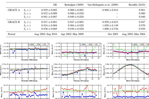
Es-Table 3.Scale factorsSof accelerometer measurements of GRACE A and B obtained from different methods in the along-track (x), cross-track (y) and radial (z) directions of the SRF.
DE Bettadpur (2009) Van Helleputte et al. (2009) Bezdˇek (2010)
GRACE A Sx(–) 0.939±0.002 0.960±0.002 0.960±0.014 0.961
Sy(–) 0.922±0.009 0.980±0.020 − 0.980
Sz(–) 0.941±0.007 0.949±0.020 − 0.940
GRACE B Sx(–) 0.931±0.001 0.947±0.002 0.950±0.015 0.947
Sy(–) 0.916±0.004 0.984±0.020 1.050±0.149 0.970
Sz(–) 0.938±0.005 0.930±0.020 1.000±0.536 0.920
Period Aug 2002–Sep 2016 Apr 2002–Mar 2009 Oct 2003 Aug 2002–Mar 2004
−1.4e−06 −1.3e−06 −1.2e−06 −1.1e−06 −1e−06 B ia s x [m s ] -2
0 5 10 15 20 25 30
November 2008 [days]
MNE EMA DE
−1.4e−06 −1.3e−06 −1.2e−06 −1.1e−06 −1e−06 B ia s x
0 5 10 15 20 25 30
February 2014 [days]
MNE EMA DE
−1.4e−06 −1.3e−06 −1.2e−06 −1.1e−06 −1e−06 B ia s x
0 5 10 15 20 25 30
March 2015 [days]
MNE EMA DE
2.72e−05 2.73e−05 2.74e−05 2.75e−05 B ia s y
0 5 10 15 20 25 30
November 2008 [days]
2.92e−05 2.93e−05 2.94e−05 2.95e−05 2.96e−05 B ia s y
0 5 10 15 20 25 30
February 2014 [days]
2.84e−05 2.88e−05 2.92e−05 2.96e−05 B ia s y
0 5 10 15 20 25 30
March 2015 [days]
−8e−07 −6e−07 −4e−07 B ia s z
0 5 10 15 20 25 30
November 2008 [days]
−8e−07 −6e−07 −4e−07 B ia s z
0 5 10 15 20 25 30
February 2014 [days]
−8e−07 −6e−07 −4e−07 B ia s z
0 5 10 15 20 25 30
March 2015 [days]
[m s ] -2 [m s ] -2 [m s ] -2 [m s ] -2 [m s ] -2 [m s ] -2 [m s ] -2 [m s ] -2
B B B
Figure 2.Comparison of daily biases of acceleration measurements of GRACE A during low (November 2008), high (February 2014) and medium (March 2015) solar activity. In these figures, MNE represents the multi-step numerical estimation (blue), DE indicates the dynamic estimation (red) and EMA stands for the empirical model approach (green). Results are presented in the along-track (x), cross-track (y) and radial (z) directions of the SRF. Note that the scale of theyaxis differs due to varying biases along the three axes.
pecially in the radial direction, biases show larger variations with time while comparing to the along-track and cross-track directions. Moreover, an offset is found between the calibra-tion parameters obtained from MNE and other approaches; however, the reason for this difference remains unclear.
Based on the numerical results, one can see that cali-bration parameters obtained from MNE and DE are fairly similar in the along-track and cross-track directions. The offset between along-track calibration parameters obtained from EMA, compared to other methods, is caused by the dependency of its results on the density derived from em-pirical models (Doornbos, 2012). This emem-pirical approach will likely become more realistic by introducing a horizontal wind model to the calculation of the satellite’s relative veloc-ities within drag estimations (Eq. 9; Sutton, 2008). Moreover, Mehta et al. (2014) found that an improved understanding of the gas–surface interactions impacts the drag coefficient and hence yields more realistic neutral density for the GRACE
satellites. The results obtained in this study confirm the order of magnitude of biases in all three directions, which are de-rived by Bezdˇek (2010, Fig. 14) for 1.5 years at the beginning of the mission.
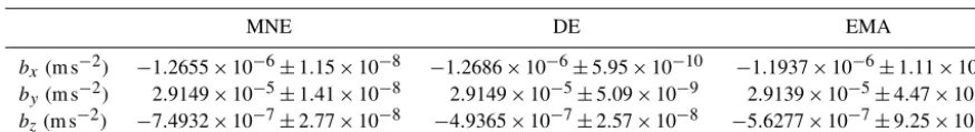
[image:8.612.52.546.92.421.2]Table 4.Mean values and standard deviations of biasesbof GRACE A during March 2015 obtained from the multi-step numerical estimation (MNE), the dynamic estimation (DE) and the empirical model approach (EMA) in the along-track (x), cross-track (y) and radial (z) directions of the SRF.
MNE DE EMA
bx(m s−2) −1.2655×10⁻⁶±1.15×10⁻⁸ −1.2686×10⁻⁶±5.95×10⁻¹⁰ −1.1937×10⁻⁶±1.11×10⁻⁹
by(m s−2) 2.9149×10⁻⁵±1.41×10⁻⁸ 2.9149×10⁻⁵±5.09×10⁻⁹ 2.9139×10⁻⁵±4.47×10⁻¹⁰
bz(m s−2) −7.4932×10⁻⁷±2.77×10⁻⁸ −4.9365×10⁻⁷±2.57×10⁻⁸ −5.6277×10⁻⁷±9.25×10⁻¹⁰
4.2 Thermospheric neutral density estimation
By applying daily biases and the constant scale factors on raw accelerometer measurements, corresponding calibrated time series are computed. The calibrated accelerometer mea-surements obtained from the three applied calibration proce-dures (Sect. 3.1, 3.2, and 3.3) are used to compute thermo-spheric neutral density profiles in the along-track direction (Sect. 3.4). In addition, the derived densities are compared to two different empirical models NRLMSISE-00 (Picone et al., 2002) and Jacchia–Bowman 2008 (Bowman et al., 2008). For evaluating the accelerometer-based densities resulting from this study, density sets by Sutton (2008), and more recently estimated densities from Mehta et al. (2017), both available between 2002 and 2010, are taken into account3. Through-out this study, the densities are not normalized to a con-stant altitude, which is done for example in Lei et al. (2012), since such a normalization needs an assumption about verti-cal changes in the thermospheric density.
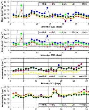
Daily averages of along-track densities during three par-ticular months with high, medium and low solar activity are presented in Fig. 3. Average densities during Novem-ber 2008 vary about 2×10⁻¹³kg m−3, which is more than one order of magnitude less than those during high (3× 10⁻¹²kg m−3) or medium (2×10⁻¹²kg m−3) solar activity. Independent of the solar activity, empirical densities obtained from NRLMSISE-00 coincide best with the densities calcu-lated from EMA. This is due to the fact that the NRLMSISE-00 model is already used for estimating the calibration pa-rameters (see Sect. 3.3.1). Densities obtained from MNE and DE, however, are independent of empirical density models and agree well during high and medium solar activity. During high solar activity the stability of the calibration parameters increases due to the intensity of the non-gravitational forces measured by the accelerometer as stated by Van Helleputte et al. (2009). A validation of densities derived in this study is possible when taking daily mean densities by Sutton (2008) and Mehta et al. (2017) in November 2008 into ac-count. Relative to Sutton (2008), the root mean square dif-ference (RMSD) of the approaches used in this study are 3.7×10⁻¹⁴kg m−3 (MME), 2.4×10⁻¹⁴kg m−3 (DE) and 2.2×10⁻¹³kg m−3 (EMA), whereas the RMSD relative to
Mehta et al. (2017) are 5.3×10⁻¹³kg m−3 (MME), 1.8×
3http://tinyurl.com/densitysets; last access: 16 May 2018
10−13kg m−3(DE) and 3.8×10⁻¹³kg m−3(EMA). During
this period, the DE approach is found to be the most suitable method to calibrate accelerometer measurements in order to derive thermospheric neutral densities. Since DE-derived densities are closer to those of Sutton (2008) than to the re-cently computed densities by Mehta et al. (2017), we confirm that an improved drag estimation as performed by (Mehta et al., 2017) affects the density estimates. For example, using an effective energy accommodation coefficient is expected to increase the densities up to 20 % (Mehta et al., 2013), and a better understanding of the gas–surface interaction will lead to further improvements (Mehta et al., 2017).
In addition to daily mean densities, the along-track den-sities on 1 November 2008 are presented in Fig. 4, whose results indicate that the general pattern is the same as the pattern of densities obtained in this study. Dominant peaks with a 1.5 h period are found to be evident that is related to the orbital period of approximately 15 revolutions per day. DE-derived densities are found to be closest to Sutton (2008) densities with a RMSD of 8.2×10⁻¹²kg m−3. In compari-son, the RMSD based on density sets by Mehta et al. (2017) is 2.5×10⁻¹¹kg m−3 for densities by Sutton (2008), and 2.1×10⁻¹¹kg m−3for DE-derived densities. We observe that DE-derived densities for this day are closer to those pub-lished by Mehta et al. (2017) than those in Sutton (2008).
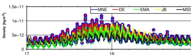
On 17 and 18 March 2015, thermospheric densities reach a maximum due to a strong solar event (St. Patrick’s Day storm). Along-track densities during these days are presented in Fig. 5. Accelerometer-based densities (MNE, DE, EMA) show stronger reactions to this storm of up to 1.2×10⁻¹¹kg m−3 compared to empirically modeled
den-sities of NRLMSISE-00 (0.6×10⁻¹¹kg m−3) and JB2008 (0.9×10⁻¹¹kg m−3) due to variations within the atmo-spheric composition affecting the atmoatmo-spheric density and thus accelerometer measurements. However, JB2008 mod-eled densities seem to better represent the solar event than NRLMSISE-00 even though the maximum is delayed. The temporal resolution of input parameters such asF10.7index
0 1e−13 2e−13 3e−13 4e−13 5e−13
Mean
density
[kg m
]
-3
0 5 10 15 20 25 30
November 2008 [days]
MNE DE EMA JB MSIS
0 1e−13 2e−13 3e−13 4e−13 5e−13
0 5 10 15 20 25 30
November 2008 [days]
MNE DE EMA Mehta Sutton
0 1e−12 2e−12 3e−12 4e−12 5e−12
0 5 10 15 20 25 30
February 2014 [days]
MNE DE EMA JB MSIS
0 1e−12 2e−12 3e−12 4e−12 5e−12
0 5 10 15 20 25 30
March 2015 [days]
MNE DE EMA JB MSIS
Mean
density
[kg m
]
-3
Mean
density
[kg m
]
-3
Mean
density
[kg m
]
[image:10.612.145.452.65.442.2]-3
Figure 3.Daily average of along-track densities during November 2008 (low), February 2014 (medium) and March 2015 (high solar activity). Density obtained from calibrated accelerometer measurements: multi-step numerical estimation (MNE, blue), dynamic estimation (DE, red) and empirical model approach (EMA, green). Density obtained from empirical density models are shown as NRLMSISE-00 (MSIS, black) and Jacchia–Bowman 2008 (JB, yellow). Density sets by Mehta et al. (2017) (grey) and Sutton (2008) (light red) are available in 2008. Note that the scale of theyaxis differs due to a strong variation in solar activity.
empirically modeled densities, in particular during strong so-lar events.
4.3 Empirical density corrections for NRLMSISE-00 In the following, the accelerometer-based densitiesρcal are
used to estimate empirical corrections for NRLMSISE-00 densities ρ in terms of scale factorss=ρcalρ−1 similar to
Doornbos et al. (2009). Mean empirical corrections during November 2008, February 2014 and March 2015 along the orbit of GRACE A are presented in Fig. 6. Since densities de-rived from EMA coincide with NRLMSISE-00 densities (see Fig. 3), empirical corrections are not estimated for EMA.
In November 2008, the MNE-based empirical corrections are less reliable due to less stable calibration parameters re-sulting from this approach during periods of a low
signal-to-noise ratio. Due to the similarity of the calibration parameters derived from MNE and DE during high and medium solar ac-tivity, the density corrections obtained from both approaches are found to be similar with mean values of 1.11 (MNE) and 1.12 (DE) in March 2015, and in February 2014 the mean values are found to be 0.99 (MNE) and 0.97 (DE). During the St. Patrick’s Day storm (17 and 18 March 2015), the mean empirical corrections increase on 17 March, and decrease af-terwards due to the delayed and weakened maximum in the empirical thermospheric densities (see also Fig. 5).
0 1e−13 2e−13 3e−13 4e−13
D
e
n
s
it
y
[
k
g
m
]
-3
1.0 1.2 1.4 1.6 1.8 2.0
November 2008 [days]
MNE EMA JB MSIS
0 1e−13 2e−13 3e−13 4e−13
1.0 1.2 1.4 1.6 1.8 2.0
November 2008 [days]
DE EMA Mehta Sutton
D
e
n
s
it
[k
g
m
]
-3
[image:11.612.142.454.67.248.2]y
Figure 4.Along-track densities on 1 November 2008. Density obtained from calibrated accelerometer measurements: multi-step numerical estimation (MNE, blue), dynamic estimation (DE, red) and empirical model approach (EMA, green). Density obtained from empirical density models: NRLMSISE-00 (MSIS, black) and Jacchia–Bowman 2008 (JB, yellow). Densities by Mehta et al. (2017) (grey) and Sutton (2008) (light red).
0 5e−12 1e−11 1.5e−11
17 18 19
March 2015 [days]
MNE DE EMA JB MSIS
Density
[kg
m
]
-3
Figure 5.Along-track densities during the St. Patrick’s Day storm (17 and 18 March 2015). Density obtained from calibrated accelerometer measurements: multi-step numerical estimation (MNE, blue), dynamic estimation (DE, red) and empirical model approach (EMA, green). Density obtained from empirical density models: NRLMSISE-00 (MSIS, black) and Jacchia–Bowman 2008 (JB, yellow).
approximately close to 1. Overestimated model densities dur-ing low solar activity have also been reported in Doornbos (2012), and we confirm that empirical density models per-form well only during moderate conditions.
Since the necessity of correcting empirical thermospheric neutral density models is evident, we provide global empir-ical corrections on a daily basis, which can be used to scale model-derived neutral density estimations for the altitude of ∼400 km. The corrections can likely be used for the whole altitude range of∼300–600 km, since the altitude-dependent changes in neutral density is close to linear. Empirical cor-rections on 2 March 2015, along the orbit of GRACE A, are presented in Fig. 7. Due to the similarity of the calibration parameters derived from MNE and DE, the density correc-tions obtained from both approaches are found to be similar on this day with mean values of 1.21 (MNE) and 1.24 (DE). Additionally, a spatial representation of the corrections, which are estimated for the NRLMSISE-00 empirical model along the orbit of GRACE A on 2 March 2015, are shown on the left column of Fig. 8. The empirical corrections derived
from MNE and DE indicate that NRLMSISE-00 neutral den-sities need to be increased by 22 % on average on this day.
In order to derive global patterns of differences between GRACE densities and model output, as GRACE does not exactly repeat its daily tracks, daily density scales (s=
ρcalρ−1) are first estimated by scaling the GRACE-derived
[image:11.612.144.453.321.410.2]0.0 0.5 1.0 1.5 2.0
0 5 10 15 20 25 30
November 2008 [days]
MNE DE
0.0 0.5 1.0 1.5 2.0
0 5 10 15 20 25 30
February 2014 [days]
MNE DE
0.0 0.5 1.0 1.5 2.0
Mean emp. corr. [−]
0 5 10 15 20 25 30
March 2015 [days]
MNE DE
Mean emp. corr. [−]
[image:12.612.146.453.66.354.2]Mean emp. corr. [−]
Figure 6.NRLMSISE-00 daily mean empirical corrections (emp. corr.) of GRACE A during November 2008 (low), February 2014 (medium) and March 2015 (high solar activity). Densities obtained from calibrated accelerometer measurements of the multi-step numerical estimation (MNE, blue) and the dynamic estimation (DE, red).
0 1 2 3
Emp. corr. [−]
2.0 2.2 2.4 2.6 2.8 3.0
March 2015 [days]
MNE DE
Figure 7.NRLMSISE-00 empirical corrections along the orbit of GRACE A on 2 March 2015. Densities obtained from calibrated ac-celerometer measurements of the multi-step numerical estimation (MNE, blue) and the dynamic estimation (DE, red).
loss of spatial resolution. Indeed, we find daily analysis to be an appropriate balance between temporal and spatial resolu-tion. However, we have not carried out a formal optimization, since it was out of the scope of the present paper.
From the average cross-track spacing, we found that a spherical harmonic degree of 11 could be resolved, i.e., fixing the maximum degree to 10 is appropriate. The daily spheri-cal harmonic coefficients are estimated using a least squares estimation. Numerical problems are not expected, since the analysis of the normal equation matrix yields a condition number below 103. The scale correction fields are then syn-thesized on a 1◦×1◦grid using the coefficients of up to
[image:12.612.143.454.415.509.2]−60˚ −60˚
−30˚ −30˚
0˚ 0˚
30˚ 30˚
60˚ 60˚
0˚ 0˚
0˚ 0˚
0.8 1.0 1.2 1.4 1.6
−60˚ −60˚
−30˚ −30˚
0˚ 0˚
30˚ 30˚
60˚ 60˚
0˚ 0˚
0˚ 0˚
0.8 1.0 1.2 1.4 1.6
−60˚ −60˚
−30˚ −30˚
0˚ 0˚
30˚ 30˚
60˚ 60˚
0˚ 0˚
0˚ 0˚
0.8 1.0 1.2 1.4 1.6
−60˚ −60˚
−30˚ −30˚
0˚ 0˚
30˚ 30˚
60˚ 60˚
0˚ 0˚
0˚ 0˚
0.8 1.0 1.2 1.4 1.6
(a) (b)
[image:13.612.105.491.66.223.2](c) (d)
Figure 8.NRLMSISE-00 empirical corrections of GRACE A during 2 March 2015.(a, c)Corrections along the orbit.(b, d)Corrections expanded on a global grid using a least squares adjustment to obtain spherical harmonic coefficients up to degree and order 10 (synthesized up to degree and ordern=7). Densities obtained from calibrated accelerometer measurements of the multi-step numerical estimation (MNE,
a, b) and the dynamic estimation (DE,c, d).
(right column) indicate that NRLMSISE-00 neutral density simulations need to be corrected by 22 % on average during 2 March 2015.
5 Conclusions
In this study, the measurements of the SuperSTAR ac-celerometers on board the GRACE satellites are calibrated using three procedures. The multi-step numerical estimation approach is based on the numerical differentiation of kine-matic orbits, where the main challenges are the noise ampli-fication and the temporal correlation after applying a numer-ical differentiation operator. Here, similar to Bezdˇek (2010), the Savitzky–Golay filter is applied to mitigate the impact of noise and the temporal autocorrelation is reduced by fit-ting an autoregressive process within the generalized least squares estimation of the calibration parameters. In the dy-namic estimation approach, the accelerometer measurements are calibrated within a dynamic POD based on the variational equation approach (Löcher, 2011). Finally, we apply an em-pirical model approach, where the non-gravitational forces acting on the surface of the satellite are modeled. The accel-erations due to Earth radiation pressure are computed using a new model based on present satellite data and their expansion to the spherical harmonics domain. The calibration parame-ters are then obtained by applying a least squares estimation that fits GRACE observations to modeled accelerations.
The three accelerometer calibration procedures are applied successfully using constant scale factors and are found to provide largely comparable biases particularly in the along-track and cross-along-track directions. The calibration parameters computed using the dynamic estimation yields the most real-istic calibration parameters and thermospheric neutral densi-ties, likely due to the physical consistency of this approach.
Results obtained with the multi-step numerical estimation are similar to the dynamic estimation during high and medium solar activity.
Furthermore, thermospheric neutral densities derived from calibrated accelerometer measurements in the along-track di-rection of GRACE are compared to densities obtained from the empirical models NRLMSISE-00 and Jacchia–Bowman 2008. The results suggest that accelerometer-derived den-sities provide more reliable results, especially on short timescales and during strong solar events, for example dur-ing the St. Patrick’s Day storm on 17 March 2015. Hence, accelerometer-derived densities allow for the improvement of empirical density models as already stated by Doornbos (2012), and ways to integrate these while retaining high tporal resolution should be found, e.g., by estimating 24 h em-pirical correction fields at hourly or more frequent intervals. We conclude, from comparisons with densities from Sutton (2008) and recent results from Mehta et al. (2017), that den-sities estimated using the dynamic estimation fit better than those of Sutton (2008) but not as good as those of Mehta et al. (2017).
basis. These findings encourage the use of these factors to improve empirical density models.
Further efforts in satellite drag modeling will improve the empirical model approach to calibrate accelerometer mea-surements, as well as the thermospheric neutral densities es-timated from the three methods. Moreover, including a hor-izontal wind model in the empirical model approach is ex-pected to yield more realistic densities which might improve the consistency of the results. The multi-step numerical esti-mation method may be further developed through modeling the temporal correlations of accelerometer measurements.
In further studies, the empirical corrections derived from calibrated accelerometer measurements of GRACE A could be used to model densities in order to simulate non-gravitational accelerations acting on GRACE B, which con-tributes to filling data gaps during months where only one satellite provides accelerometer measurements. Other meth-ods on transferring non-gravitational accelerations of a satel-lite to a co-orbiting one are discussed in Kim and Tapley (2015).
The calibration procedures are applicable to other satellite missions carrying space-borne accelerometers as well. Com-bining the thermospheric neutral densities derived from dif-ferent calibrated accelerometers allows further improvement of empirical density models. For example, the empirical den-sity corrections at different altitudes can be used to obtain altitude profiles to correct empirical density models, which could then be used to derive accurate drag predictions for other satellites which are not equipped with an accelerome-ter, restricted to the period when the corrections are available. Besides, the assimilation of calibrated accelerometer mea-surements of various satellite missions into physical thermo-sphere/ionosphere models would likely enable an improved representation of physical processes in the atmosphere, e.g., following Matsuo et al. (2012) or Fedrizzi et al. (2012).
Data availability. The density data that were used for
Appendix A: Numerical differentiation filters
In this synthetic experiment, we apply different numerical differentiation operators to an analytical orbit. We design an analytical orbitran= [ranx,rany,ranz]
Tat timet, e.g., for the
along-track direction
ranx(t )=afxcos(2πfxt )+bfxsin(2πfxt ), (A1)
using the main frequenciesf of the true orbit derived from a fast Fourier transform and the corresponding amplitudes af andbf resulting from a least squares adjustment.
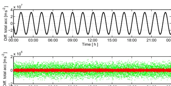
Subse-quently, various numerical derivatives can be compared with the results of the analytical derivative. Random white noise of 2 cm according to the standard deviation of the kinematic orbits has been added to the modeled orbit. The differences in analytical derivative to three different numerical derivatives are presented in Fig. A1. The numerical derivatives shown here are (1) a smoothing differentiation filter of window lengthn=10 with a kernel of [−1 . . . –1 0 1 . . . 1]·(n/2)2 of dimension 1×10 , (2) Savitzky–Golay filter with window lengthn=9 and orderm=6 of the fitted polynomial as rec-ommended by Bezdˇek (2010) and (3) Savitzky–Golay filter with settingsn=11 andm=5.
00:00 03:00 06:00 09:00 12:00 15:00 18:00 21:00 00:00 −4
−2 0 2 4x 10
7
Time [ h ]
00:00 03:00 06:00 09:00 12:00 15:00 18:00 21:00 00:00 −2
0 2x 10
6
Time [ h ]
Diff.
total
acc
[m
s
]
2-Diff.
total
acc
[m
s
]
2-Figure A1.Differences between the analytical second derivative and three numerical second derivative filters of thexcomponent of the modeled orbit in the CRF at 25 November 2003. Numerical differentiation filters: (1) smoothing differentiation filter (black), (2) Savitzky– Golay filter with settingsn=9 andm=6 (green) and (3) Savitzky–Golay filter with settingsn=11 andm=5 (red).
[image:15.612.151.450.366.517.2]Appendix B: Earth radiation pressure (ERP)
ERP is caused by albedo aalbedo, as well as thermal
emis-sion of the EarthaIR. Albedo represents the fraction of short
wavelength sunlight that is reflected back into space by the Earth’s surface or the atmosphere. The thermal emission is mainly in the infrared (IR), i.e., long wavelength radiation. ERP acceleration acting on the GRACE satellite is estimated as
aERP= 8 X
i=1
N
X
j=1
−R
jA icos(8
j
inc,i)
m
·
h
2
crd,i
3 +crs,icos(8
j
inc,i)
ni+ 1−crs,i
sj
i
, (B1)
wheresis the unit vector to the Sun,nis the unit normal on the panel,8incis the angle betweensandn,crdandcrs
rep-resent the reflectivity coefficients of the surface plates (dif-fuse and specular reflection), mis the mass of the satellite and A is the surface area of each plate. The indexi indi-cates that vectors correspond to theith plate. This means that the impact of ERP is calculated separately for each of the eight plates of GRACE and afterwards accumulated over the whole surface of the satellite. The shadow effect of the Earth onto the satellite is expressed by the coefficient ν, known as the shadow function that varies between 0 (satellite in eclipse) and 1 (full illumination of the satellite). The shadow function is estimated based on geometrical assumptions see (e.g., Montenbruck and Gill, 2012). Due to the eccentricity of the Earth’s orbit around the Sun, the solar flux will slightly change throughout the year. To account for these variations, the term 1AU2/r2 is added in Eq. (B1), where AU is the astronomical unit that represents the mean distance between the Sun and the Earth, andris the distance to the Sun. The radiation Rj originates from the Earth (satellite footprint), and even at a given time it spatially varies over the surface
−6e−08 −4e−08 −2e−08 0 2e−08
ERP
acceleration
[m s
]
-2
0 1 2 3 4 5 6
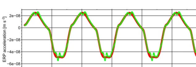
[image:16.612.139.456.514.622.2]1 Nov 2008 [h]
Figure B1.Along-track ERP accelerations on 1 November 2008. Knocke model (red) and new model with spherical harmonics (green). of the Earth. In order to calculate Rj, a model is required to provide albedo and emission coefficients corresponding to the segmentations of the satellite footprint. Knocke et al. (1988) provide a latitude-dependent model, which accounts for seasonal albedo and emission variations. In Eq. (B1),
8jinc,i is the incident angle of the ith plate with radiation originating from thejth segment, andsj is the unit vector from satellite to thejth segment (see, e.g., Doornbos, 2012, for more details).
Here, we replace the Knocke et al. (1988) model by spher-ical harmonic coefficients estimated from satellite-derived albedo and emission fields. To generate the model, we as-sume the following relation of Eq. (B2), wherelcontains the time series of albedo/emissioncnm andsnm, and a tog are
the coefficients that need to be estimated as
l(t )=a+bt+ct2+dcos(ωat )+esin(ωat )
+fcos(ωsat )+gsin(ωsat ) , (B2)
wheretis the time in modified Julian date (MJD), andωaand ωsa account for annual and semi-annual frequencies,
respec-tively. Model coefficientsa to gin Eq. (B2) are estimated using a least squares adjustment. Using the fitted coefficients ˆ
atogˆ, it is possible to calculate albedo and emission for an arbitrary time. Inserting a time in MJD in Eq. (B2) results in
snm(t )andcnm(t ), which can be used to synthesize albedo
and emission fields.
Competing interests. The authors declare that they have no conflict of interest.
Special issue statement. This article is part of the special issue “Dynamics and interaction of processes in the Earth and its space environment: the perspective from low Earth orbiting satellites and beyond”. It is not associated with a conference.
Acknowledgements. Kristin Vielberg thanks the German Academic
Exchange Service (DAAD) for the PROMOS scholarship to conduct a part of this research at Cardiff University. We thank Aleš Bezdˇek for his generous comments on the computational steps of this study. The authors are grateful to the research grant through the D-SAT project (FKZ.: 50 LZ 1402) and the TIK project (FKZ.: 50 LZ 1606) supported by the German Aerospace Center (DLR). We also acknowledge the topical editor Eelco Doornbos and the two reviewers for their helpful remarks and suggestions.
The topical editor, Eelco Doornbos, thanks two anonymous referees for help in evaluating this paper.
References
Akaike, H.: Information theory and an extension of the maxi-mum likelihood principle, Selected Papers of Hirotugu Akaike, Springer New York, 199–213, https://doi.org/10.1007/978-1-4612-1694-0_15, 1988.
Ashikhmin, M. and Shirley, P.: An anisotropic phong BRDF model, Journal of graphics tools, 5, 25–32, https://doi.org/10.1080/10867651.2000.10487522, 2000. Baarda, W: A Testing procedure for use in geodetic networks,
Pub-lications on Geodesy, Vol. 2, Nr. 5, Netherlands Geodetic Comis-sion, Delft, 1968.
Bettadpur, S.: Recommendation for a-priori Bias & Scale Parame-ters for Level-1B ACC Data (Version 2), GRACE TN-02, Center for Space Research, The University of Texas at Austin, 2009. Bettadpur, S.: Gravity Recovery and Climate Experiment: Product
Specification Document, Tech. Rep. GRACE 327-720, Center for Space Research, The University of Texas at Austin, 2012. Bezdˇek, A.: Calibration of accelerometers aboard GRACE
satellites by comparison with POD-based nongrav-itational accelerations, J. Geodyn., 50, 410–423, https://doi.org/10.1016/j.jog.2010.05.001, 2010.
Bowman, B., Tobiska, W. K., Marcos, F., Huang, C., Lin, C., and Burke, W.: A new empirical thermospheric den-sity model JB2008 using new solar and geomagnetic indices, AIAA/AAS Astrodynamics specialist conference and exhibit, 1– 19, https://doi.org/10.2514/6.2008-6438, 2008.
Bruinsma, S., Tamagnan, D., and Biancale, R.: Atmo-spheric densities derived from CHAMP/STAR accelerom-eter observations, Planet. Space Sci., 52, 297–312, https://doi.org/10.1016/j.pss.2003.11.004, 2004.
Bruinsma, S., Arnold, D., and Jäggi, A., and Sánchez-Ortiz, N.: Semi-empirical thermosphere model evaluation at low altitude with GOCE densities, J. Space Weather Spac., 7, 13 pp., https://doi.org/10.1051/swsc/2017003, 2017.
Calabia, A., Jin, S., and Tenzer, R.: A new GPS-based calibration of GRACE accelerometers using the arc-to-chord threshold un-covered sinusoidal disturbing signal, Aerosp. Sci. Technol., 45, 265–271, https://doi.org/10.1016/j.ast.2015.05.013, 2015. Case, K., Kruizinga, G., and Wu, S.-C.: GRACE Level 1B Data
Product User Handbook, Tech. Rep. JPL D-22027, Jet Propul-sion Laboratory, 2010.
Doornbos, E.: Thermospheric density and wind determination from satellite dynamics, Springer Science & Business Media, Berlin-Heidelberg, https://doi.org/10.1007/978-3-642-25129-0, 2012. Doornbos, E., Förster, M., Fritsche, B., van Helleputte,T., van den
IJssel, J., Koppenwallner, G., Lühr, H., Rees, D., Visser, P., and Kern, M.: Air density models derived from multi-satellite drag observations, in: Proceedings of ESAs second swarm international science meeting, Potsdam, Germany, 24–26 June 2009, available at: https://www.researchgate.net/ profile/Bent_Fritsche/publication/228814094_Air_Density_ Models_Derived_from_Multi-Satellite_Drag_Observations/ links/02e7e52e909d0f21d8000000.pdf, last access: 16 May 2018, 2009.
Fedrizzi, M., Fuller-Rowell, T. J., and Codrescu, M. V.: Global Joule heating index derived from thermospheric density physics-based modeling and observations, Space Weather, 10, S03001, https://doi.org/10.1029/2011SW000724, 2012.
Flechtner, F., Dobslaw, H., and Fagiolini, E.: AOD1B product de-scription document for product release 05 (Rev. 4.4, 14 Decem-ber 2015), Technical Note, GFZ German Research Centre for Geosciences Department 1, 2014.
Flury, J., Bettadpur, S., and Tapley, B. D.: Precise accelerometry onboard the GRACE gravity field satellite mission, Adv. Space Res., 42, 1414–1423, 2008.
Forootan, E., Didova, O., Kusche, J., and Löcher, A.: Comparisons of atmospheric data and reduction methods for the analysis of satellite gravimetry observations, J. Geophys. Res.-Sol. Ea., 118, 2382–2396, https://doi.org/10.1002/jgrb.50160, 2013.
Frommknecht, B.: Integrated sensor analysis of the GRACE mission, PhD thesis, Fakultät für Bauingenieur- und Vermessungswesen, Technische Universität München, https://doi.org/10.1007/3-540-29522-4_8, 2007.
Guo, J., Wan, W., Forbes, J. M., Sutton, E., Nerem, R. S., Woods, T., Bruinsma, S., and Liu, L.: Effects of so-lar variability on thermosphere density from CHAMP ac-celerometer data, J. Geophys. Res.-Space, 112, A10308, https://doi.org/10.1029/2007JA012409, 2007.
Kim, J.: Simulation study of a low-low satellite-to-satellite tracking mission, PhD thesis, University of Texas at Austin, 2000. Kim, J. and Tapley, B. D.: Estimation of non-gravitational
ac-celeration difference between two co-orbiting satellites us-ing sus-ingle accelerometer data, J. Geodesy, 89, 537–550, https://doi.org/10.1007/s00190-015-0796-2, 2015.
Klinger, B. and Mayer-Gürr, T.: The role of accelerometer data calibration within GRACE gravity field recovery: Re-sults from ITSG-Grace2016, Adv. Space Res., 58, 1597–1609, https://doi.org/10.1016/j.asr.2016.08.007, 2016.